–Brief Paper–
EXPONENTIAL STABILITY FOR MULTI-AREA POWER SYSTEMS WITH
TIME DELAYS UNDER LOAD FREQUENCY CONTROLLER FAILURES
Xu Li, Rui Wang, Shu-Nan Wu, and Georgi M. Dimirovski
ABSTRACT
This paper investigates the exponential stability problem for a class of multi-area power systems with time delays under load frequency controller failures (LFCFs). For describing the phenomenon of LFCFs, the considered multi-area power system is rewritten as a switched system with multiple time delays. By adopting the switching technique, the exponential stability conditions for multi-area power systems are developed when the controller failure frequency and the unavailability ratio of the controller are restricted. Finally, one example is given to show the applicability of the proposed method.
Key Words: Multi-area power systems, time delays, load frequency controller failure (LFCF), switched systems.
I. INTRODUCTION
In order to maintain the frequency and power inter-changes with neighborhood areas at scheduled values, load frequency control is widely used in multi-area power systems [1]. Using open communication networks is a future trend in power systems and time delays are also introduced into power systems. It is widely known that time delays can degrade the performance of a system, and may even make systems unstable [2,3]. To study the prob-lem of time delays, multi-area power systems with time delays are modeled as systems with multiple time delays and many significant results are proposed [1,4,5].
On the other hand, controller failures are often encountered in real control systems due to various rea-sons [6,7]. The first reason is that control signals may be not transmitted perfectly in the open communication net-works, or the controller itself is not available. The second reason is that we desire to suspend the controller pur-posefully from time to time when economical issues or system life is considered.
In this paper, the exponential stability problem for a class of multi-area power systems with time delays under load frequency controller failures (LFCFs) is stud-ied. First, the considered multi-area power system with
Manuscript received August 31, 2015; revised March 4, 2016; accepted June 19, 2016.
X. Li, R. Wang and S. -N. Wu are with the School of Aeronautics and Astronautics, Dalian University of Technology, Dalian 116024, China.
G. M. Dimirovski is with the School of Engineering, Dogus University, Aciba-dem, TR-34722 Istanbul, Turkey, and also with the School FEIT, St. Cyril and St. Methodius University, Karpos 2, MK-1000 Skopje, Macedonia.
Shu-Nan Wu is the corresponding author (e-mail: [email protected]). This work was supported by the NSFC under Grant 61374072.
time delays under LFCFs is modeled as a switched sys-tem with multiple time delays, which includes an unstable subsystem with LFCFs and a stable subsystem without LFCFs. Then, based on the switching technique, expo-nential stability conditions for multi-area power systems under LFCFs are proposed. Finally, an example is given to demonstrate the applicability of the proposed method.
II. PROBLEM FORMULATION
A class of multi-area power systems including n control areas can be expressed as follows [1]:
̇x(t) = Ax(t) + n ∑ i=1 Adix(t −𝜏i(t)) + F ΔPd, (1) where x(t) =[x1(t) · · · xn(t)]T, ΔPd =[ΔPd1 · · · ΔPdn]T, xi(t) =[Δfi ΔPmi ΔPvi ∫ ACEi ΔPtiei]T, A = ⎡ ⎢ ⎢ ⎣ A11 · · · A1n ⋮ ⋱ ⋮ An1 · · · Ann ⎤ ⎥ ⎥ ⎦, F = ⎡ ⎢ ⎢ ⎣ F1 · · · 0 ⋮ ⋱ ⋮ 0 · · · Fn ⎤ ⎥ ⎥ ⎦, Aii= ⎡ ⎢ ⎢ ⎢ ⎢ ⎢ ⎢ ⎢ ⎢ ⎣ −Di mi 1 mi 0 0 −1 mi 0 − 1 Tchi 1 Tchi 0 0 − 1 TgiRi 0 − 1 Tgi 0 0 𝛽i 0 0 0 1 2𝜋 n ∑ j=1,j≠i Tij 0 0 0 0 ⎤ ⎥ ⎥ ⎥ ⎥ ⎥ ⎥ ⎥ ⎥ ⎦ ,
Aij= ⎡ ⎢ ⎢ ⎢ ⎢ ⎢ ⎣ 0 0 0 0 0 0 0 0 0 0 0 0 0 0 0 0 0 0 0 0 −2𝜋Tij 0 0 0 0 ⎤ ⎥ ⎥ ⎥ ⎥ ⎥ ⎦ , Adi = ⎡ ⎢ ⎢ ⎢ ⎢ ⎣ 0 · · · 0 · · · 0 ⋮ ⋱ ⋮ ⋱ ⋮ 0 · · · −BiKiCi · · · 0 ⋮ ⋱ ⋮ ⋱ 0 0 · · · 0 · · · 0 ⎤ ⎥ ⎥ ⎥ ⎥ ⎦ , Ki= [KPiKIi], Bi= [ 0 0 1 Tgi 0 0 ]T , Ci= [ 𝛽i 0 0 0 1 0 0 0 1 0 ] , Fi= [ −1 mi 0 0 0 0 ]T , Tij= Tji, i, j = 1, 2..., n, i ≠ j,
Δfi, ΔPmi, ΔPvi, ΔPdi, ΔPtiei are the deviation of
fre-quency, generation mechanical output, valve position, load, net tie-line power exchange, respectively. ACEiand ∫ ACEiare the area control error of the ith area and its
time integration, respectively. For the ith area, mi, Di,
Tchi, Tgi,𝛽iand Ridenote the moment of inertia of the generator, generator damping coefficient, time constant of the governor, time constant of the turbine, the fre-quency bias factor and speed drop, respectively. Tijis the tie-line synchronizing coefficient between the ith and jth control area. KPi and KIi are proportional and integral gains of PI controller, respectively.𝜏i(t) (i = 1, 2..., n) are the time delays that satisfy 0≤ 𝜏(t) ≤ hi, ̇𝜏i(t)≤ di< 1.
For convenience, the area numbers of failure con-trollers are described by a subset Ωf, where Ωf ⊂ Ω = {1, 2, · · · , n} and the outputs of the failure controllers sat-isfy KPi = KIi = 0 (∀i ∈ Ωf). Then, system (1) under
LFCFs can be described by the following switched delay system: ̇x(t) = Ax(t) + n ∑ i=1 E𝜎(t),ix(t −𝜏i(t)) + F ΔPd, (2) where 𝜎(t) ∶ [0, +∞) ∈ {1, 2} is the switching signal which is a piecewise constant function; when𝜎(t) = 1, the first subsystem is activated and there are no LFCFs; when𝜎(t) = 2, it means that LFCFs appear. Ei,j (i = 1, 2, j = 1, ...n) are constant matrices that hold
E1,j = Adj(∀j ∈ Ω), E2,j=
{
0, ∀j ∈ Ωf,
Adj, ∀j ∈ Ω∕Ωf. (3)
In order to obtain our main results, the following defini-tions are introduced.
Definition 1 ([7]). For any t > t0 ≥ 0, let Nf(t0, t) and Tu(t0, t) denote the number of LFCF and the total time interval of LFCF in time interval [t0, t), respectively.
Ff(t0, t) = Nf(t0, t)∕(t−t0) and Tu(t0, t)∕(t−t0) denote the controller failure frequency and the unavailability ratio of the controller in time interval [t0, t), respectively.
III. STABILITY ANALYSIS Consider the following delay system
̇x(t) = Ax(t) + n ∑ i=1 E1,ix(t −𝜏i(t)), x(t) =𝜙(𝜃), 𝜃 ∈ [−h, 0], (4)
where x(t) is the state vector, A, E1,i (i = 1, 2, ..., n) are constant matrices,𝜏i(t) (i = 1, 2, ..., n) satisfy 0 ≤ 𝜏i(t)≤
hi, ̇𝜏i(t) ≤ di < 1, 𝜙(𝜃) denotes the continuously
dif-ferentiable vector-valued initial function of𝜃 ∈ [−h, 0],
h = max{h1, ..., hn}.
Choose the Lyapunov functional of the following form: V1(t) = xT(t)P1x(t) + n ∑ i=1∫ t t−𝜏i(t) xT(s)e𝛼1(s−t)R 1,ix(s)ds + n ∑ i=1∫ 0 −hi∫ t t+𝜃 ̇x T (s)e𝛼1(s−t)Z 1,i̇x(s)dsd𝜃, (5)
where P1, R1,i, Z1,i (i = 1, 2, ..., n) are positive definite matrices to be determined.
Lemma 1. For given constants𝛼1> 0, hi≥ 0, di< 1 (i =
1, 2, ..., n), if there exist positive definite symmetric matri-ces P1 > 0, R1,i > 0, Z1,i > 0 (i = 1, 2, ...n), and any matrices Ni (i = 1, 2, ...n) with appropriate dimensions such that the following linear matrix inequality (LMI) holds: ⎡ ⎢ ⎢ ⎢ ⎢ ⎢ ⎣ Δ11 · · · Δ1(n+1) · · · Δ1(2n+1) ⋮ ⋱ ⋮ ⋱ ⋮ ∗ · · · Δ(n+1)(n+1) · · · 0 ⋮ ⋱ ⋮ ⋱ ⋮ ∗ · · · ∗ · · · Δ(2n+1)(2n+1) ⎤ ⎥ ⎥ ⎥ ⎥ ⎥ ⎦ < 0, (6)
then, along the trajectory of system (4), we have V1(t)<
e−𝛼1(t−t0)V
Δ11= 2ATP1+𝛼P1+ n ∑ i=1 (R1,i+ Ni+ NiT + hiATZ1,iA), Δ1j= P1E1,j−1− Nj−1 + n ∑ i=1 hiATZ 1,iE1,j−1(j = 2, · · · , n + 1), Δ1(n+1+m) = CmNm, Cm= 1 𝛼1 (e𝛼1hm− 1) (m = 1, · · · , n), Δjj= −(1 − dj)e−𝛼1hjR1,j−1 + n ∑ i=1 [hi(E1,j−1)TZ1,iE1,j−1] (j = 2, · · · , n + 1), Δll= −Cl−(n+1)Z1,l−(n+1)(l = n + 2, · · · , 2n + 1), Δgk= n ∑ i=1 hi(E1,g−1)TZ1,iE1,k−1 (g = 2, · · · , n, g < k ≤ n + 1).
Proof. From the Leibniz-Newton formula, for matrices
Ni(i = 1, 2, ..., n), it is true that 2 n ∑ i=1 x(t)Ni× [x(t) − x(t −𝜏i(t)) − ∫ t t−𝜏i(t) ̇x(s)ds] = 0. (7)
Combining (4), (5) and (7), we have ̇V1(t)+𝛼1V1(t)≤
𝜁(t)TΔ𝜁(t), where 𝜁(t) = [xT(t) xT(t −𝜏 1(t)) · · · xT(t −𝜏n(t))]T, Δ = ⎡ ⎢ ⎢ ⎣ Δ11+∑ni=1NiCiZ−1 1,iNiT · · · Δ1(n+1) ⋮ ⋱ ⋮ ∗ · · · Δ(n+1)(n+1) ⎤ ⎥ ⎥ ⎦,
Ci, Δij(i, j = 1, · · · , n + 1) are defined in Lemma 1. By using the Schur complement lemma, it is clear that (6) is equivalent to Δ< 0. Based on (6) and (7), it is clear that
̇V1(t) +𝛼V1(t)< 0 holds. Integrating this inequality gives
inequality (7). The proof is completed. Consider the following delay system:
̇x(t) = Ax(t) + n ∑ i=1 E2,ix(t −𝜏i(t)), x(t) =𝜙(𝜃), 𝜃 ∈ [−h, 0], (8)
where x(t) is the state vector, A, E2,i (i = 1, 2, ..., n) are constant matrices, 𝜏i(t) (i = 1, 2, ..., n) satisfy 0 ≤ 𝜏i(t) ≤ hi, ̇𝜏i(t) ≤ di < 1, 𝜙(𝜃) denotes contin-uously differentiable vector-valued initial function of
𝜃 ∈ [−h, 0], h = max{h1, ..., hn}.
Choose the Lyapunov functional of the following form V2(t) = xT(t)P2x(t), + n ∑ i=1∫ t t−𝜏i(t) xT(s)e𝛼2(t−s)R 2,ix(s)ds, + n ∑ i=1∫ 0 −hi∫ t t+𝜃 ̇x T(s)e𝛼2(t−s)Z 2,i̇x(s)dsd𝜃, (9)
where P2, Q2,i, R2,i (i = 1, 2, ..., n) are positive definite matrices to be determined.
Lemma 2. For given constants𝛼2> 0, hi≥ 0, di< 1 (i =
1, 2, ..., n), if there exist positive definite symmetric matri-ces P2 > 0, R2,i > 0, Z2,i > 0 (i = 1, 2, ..., n), and any matrices Mi(i = 1, 2, ..., n) with appropriate dimensions such that the following LMI holds:
⎡ ⎢ ⎢ ⎢ ⎢ ⎢ ⎣ Φ11 · · · Φ1(n+1) · · · Φ1(2n+1) ⋮ ⋱ ⋮ ⋱ ⋮ ∗ · · · Φ(n+1)(n+1) · · · 0 ⋮ ⋱ ⋮ ⋱ ⋮ ∗ · · · ∗ · · · Φ(2n+1)(2n+1) ⎤ ⎥ ⎥ ⎥ ⎥ ⎥ ⎦ < 0, (10)
then, along the trajectory of system (8), we have V2(t)<
e𝛼2(t−t0)V 2(t0), where Φ11= 2ATP2−𝛼2P2+ n ∑ i=1 (R2,i+ Mi+ MiT + hiATZ2,iA), Φ1j = P2E2,j−1− Mj−1 + n ∑ i=1 hiATZ2,iE2,j−1(j = 2, · · · , n + 1), Φ1(n+1+m)= ̄CmMm, ̄Cm= 1 𝛼2 (1 − e−𝛼2hm) (m = 1, · · · , n), Φjj= −(1 − dj)R2,j−1 + n ∑ i=1 [hi(E2,j−1)TZ2,iE2,j−1](j = 2, · · · , n + 1), Φll= − ̄Cl−(n+1)Z2,l−(n+1)(l = n + 2, · · · , 2n + 1), Φgk= n ∑ i=1 hi(E2,g−1)TZ2,iE2,k−1 (g = 2, · · · , n, g < k ≤ n + 1).
Proof. Similar to the proof of Lemma 1.
Based on Lemma 1 and Lemma 2, the main result of this paper is given as follows.
Theorem 1. For given constants𝛼1 > 0, 𝛼2 > 0, hi ≥ 0,
di < 1 (i = 1, 2, ..., n), if there exist positive definite
symmetric matrices Pi > 0, Ri,j > 0, Zi,j > 0 (i = 1, 2, j = 1, 2, ..., n), and any matrices Ni, Mi(i = 1, 2, ..., n) with appropriate dimensions such that LMIs (6) and (10) hold, then under the switching signal 𝜎(t), system (2) is exponentially stable, when the following inequalities hold: Tu(0, t) t ≤ 𝛼1−𝛼∗ 𝛼1+𝛼2 , 𝛼∗∈ (0, 𝛼 1), (11) and Ff(0, t) ≤ 𝛼 2 ln𝜇 + (𝛼1+𝛼2)h, 𝛼 ∈ (0, 𝛼 ∗), (12) where 𝜇 ≥ 1 satisfies Pl ≤ 𝜇Pm, Rl,i ≤ 𝜇Rm,i, Zl,i ≤ 𝜇Zm,i(i = 1, 2, ..., n, {l, m} = {1, 2}, {2, 1}).
Proof. Construct the following piecewise Lyapunov
functional:
V (t) =
{
V1(t), t ∈ [t2j, t2j+1),
V2(t), t ∈ [t2j+1, t2j+2), (13) where j=0,...n; V1(t) and V2(t) are defined in (5) and (9),
respectively. It can be seen that
V1(t)≤ 𝜇V2(t), V2(t)≤ e(𝛼1+𝛼2)h𝜇V1(t). (14)
From Lemma 1, Lemma 2, (13) and (14), for any t ∈ [t2j, t2(j+1)), it holds that
V (t)< 𝜇2Nf(0,t)e(𝛼1+𝛼2)hNf(0,t)
× e−𝛼1(t−Tu(t))+𝛼2Tu(t)V 1(0).
(15)
From (11) and (12), we can obtain
−𝛼1(t − Tu(t)) +𝛼2Tu(t)≤ −𝛼∗t (16)
and
𝜇2Nf(0,t)e(𝛼1+𝛼2)hNf(0,t)≤ e𝛼t. (17)
Applying (16) and (17) to (15), it is obvious that
V (t)< e−(𝛼∗−𝛼)t
V1(0). (18) The proof is completed.
IV. EXAMPLE
In this section, system (1) including two control areas is considered. The parameters of the two-area power system are from [1]. Since the net tie-line power exchanges between each control area satisfy∑2i=1ΔPtiei=
0, the order of system (1) can be reduced by one. We select
K1 = K2 = [0.2 0.6]. Based on the results in [1], it is
known that system (1) is stable for𝜏1(t) =𝜏2(t) = 0.833 + 0.5sin(t), d1= d2 = 0.5. For 𝛼1= 0.1, 𝛼2= 0.15, 𝜇 = 1.1, Ω = {1, 2} and Ωf = {2}, the feasible solutions of LMIs (6) and (10) can be obtained. By setting𝛼∗ = 0.05 and
𝛼 = 0.0044, we have Tu(0,t)
t ≤ 0.2 and Ff(0, t) ≤ 0.0084.
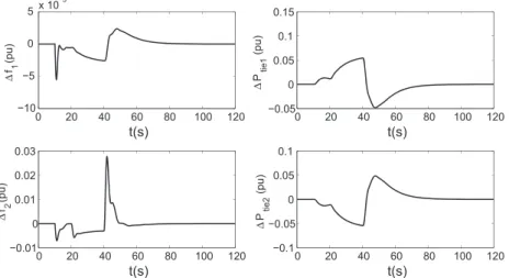
We assume𝜙(0) = 0 and add ΔPdi(i ∈ {1, 2}) = 0.1(pu) to system (2) at t = 10s. Based on the above discussions, the following switching signal is chosen:
𝜎1(t) =
{
1 t ∈ [0, 20)⋃[40, 120), 2 t ∈ [20, 40).
From Fig. 1, it is clear that the trajectories of the considered power system under𝜎1(t) can still converge to zero.
V. CONCLUSION
This paper has studied the exponential stability problem for a class of multi-area power systems with time delays under LFCFs. To deal with the problem, the considered multi-area power system is modeled as a switched delay system. Then, sufficient conditions which can guarantee the exponential stability of multi-area power systems with time delays under LFCFs are posed. Finally, the given example shows that the pro-posed method is effective and applicable.
REFERENCES
1. Jiang, L., W. Yao, J. Wen, S. Cheng, and Q. Wu, “Delay-dependent stability for load frequency con-trol with constant and time-varying delays,” IEEE
Trans. Power Syst., Vol. 27, No. 2, pp. 932–941
(2012).
2. Zeng, H., Y. He, M. Wu, and J. She, “New results on stability analysis for systems with discrete distributed delay,” Automatica, Vol. 60, pp. 189–192 (2015). 3. Milano, F. and M. Anghel, “Impact of time delays on
power system stability,” IEEE Trans. Circuits Syst.
I-Regul. Pap., Vol. 59, No. 4, pp. 889–900 (2012).
4. Bevrani, H. and T. Hiyama, “On load-frequency reg-ulation with time delays: design and real-time imple-mentation,” IEEE Trans. Energy Convers., Vol. 24, No. 1, pp. 292–300 (2009).
5. Zhang, C., L. Jiang, Q. Wu, Y. He, and M. Wu, “Delay-dependent robust load frequency control for time delay power systems,” IEEE Trans. Power Syst., Vol. 28, No. 3, pp. 2192–2201 (2013).
6. Zhai, G. and H. Lin, “Controller failure time analysis for symmetric H∞control systems,” Int. J. Control, Vol. 77, No. 6, pp. 598–605 (2004).
7. Sun, X., G. Liu, D. Rees, and W. Wang, “Stability of systems with controller failure and time-varying delay,” IEEE Trans. Autom. Control, Vol. 53, No. 10, pp. 2391–2396 (2008).