APPLICATION OF GREY RELATIONAL ANALYSIS WITH
FUZZY AHP TO FMEA METHOD
GRİ İLİŞKİ ANALİZİ VE BULANIK ANALİTİK HİYERARŞİ SÜRECİ YÖNTEMİNİN HMEA ANALİZİNDE UYGULANMASI
Çiğdem SOFYALIOĞLU
(1), Şule ÖZTÜRK
(2)Celal Bayar University
Business Administration Department, Quantitative Methods Program (1)[email protected], (2)[email protected]
ABSTRACT: The purpose of this study is to compare three different methods for
prioritizing failure modes in a design FMEA study. These methods are traditional approach, Grey Relational Analysis (GRA- under the assumption of risk factors having equal weights) and integration of Grey Relational Analysis and Fuzzy Analytic Hierarchy Process (FAHP) -to estimate weights for the risk factors-. According to the findings, integration of Grey Relational Analysis and fuzzy AHP revealed a difference in prioritizing failure modes from the methods with the assumption of equal weights. Because this method eliminates some of the shortcomings of the traditional approach, it is a useful tool in identifying the high-priority failure modes.
Keywords: FMEA; RPN; Grey Relational Analysis; Fuzzy AHP JEL Classification: C00
ÖZET: Bu çalışmanın amacı bir tasarım HMEA uygulamasında, hata türlerini önceliklendirmede kullanılabilecek üç farklı yöntemi karşılaştırmaktır. Bu yöntemler; geleneksel HMEA risk öncelik sıralaması, Gri İlişki Analizi (risk faktörlerinin ağırlıklarının eşit olduğu varsayımı altında) ve risk faktörlerine farklı ağırlıklar vermek üzere Gri İlişki Analizi ve Bulanık Analitik Hiyerarşi Prosesi (BAHP) yöntemlerinin birlikte uygulanmasıdır. Elde edilen bulgulara göre Gri İlişki Analizi ve bulanık AHP birlikte kullanıldığında oluşan sıralamanın, ağırlıkların eşit olduğu varsayımına dayanan sıralamaya göre farklı olduğu gözlemlenmiştir. Bu yöntemin, geleneksel yaklaşımın bazı sakıncalarını giderebildiği için, öncelikli hata türlerini belirlemede etkin bir yöntem olduğu öne sürülebilir.
Anahtar Kelimeler: HMEA; RÖP; Gri İlişkisel Analiz; Bulanık AHP
1. Introduction
In developing and competitive market conditions, fixing the problem after it occurred may not satisfy most of the customers. That is why preventive measures for the potential failures become so valuable for the firms. If preventive measures are not taken, cost of a failure mode in a component can be added to the manufacturing cost. Therefore, preventive measures are necessary to decrease manufacturing costs. On the other hand, preventive measures are not only valuable in decreasing costs, but also in providing customer satisfaction by preventing failures before they reach to the customers.
Failure mode and effect analysis (FMEA) is not only a method that aims to show potential failure modes, it also shows the causes and the effects of these modes. The FMEA methodology is also used in identifying controls in order to reduce the
likelihood of occurrence of the failures (FMEA Ford Motor Company, 2008: 7-66. pp). From the manufacturing perspective, FMEA methodology studies the equipments and the occasions in which the equipments can malfunction. It also studies the possible problems and their effects in the manufacturing process (Baysal
et al., 2002: 83-90.pp.). FMEA helps to identify potential failures in the early
stages (Erginel, 2008 ; Baysal et al., 2002; Chang et al., 2001; Chin et al., 2008; Öndemir et al., 2004; Wang et al.). This technique was firstly used by NASA in 1960s. The first applications in automotive industry were held by Ford Motor Company (Öndemir et al., 2004; Keskin and Özkan, 2009; Erginel, 2008). This method enables to identify and analyze the effects of the failure modes as the way customers perceive them (Baysal et al., 2002).
In the FMEA application, possible failure modes, possible effects of these failure modes, priorization of these failure modes and the corrective measures are identified with the help of a template. Failure mode is defined as a system, process or a component which impedes to reach the expected results. A failure mode is not only limited in its own department. A failure mode in a department may be the reason of a failure mode in another department. The effect of a failure mode is defined as the results of a failure mode as the way a customer perceives them (Chin et al., 2008). Types of FMEA are as following;
System FMEA: This type of FMEA aims to identify potential failure modes in the system functions by analyzing the systems, sub-systems and interactions of these systems with each other.
Process FMEA: This type of FMEA aims to identify and prevent possible failures, their causes and effects during a process.
Design FMEA: This type of FMEA aims to identify and prevent possible failures, their causes and effects during a new product design.
In this study, a design FMEA data of a heating equipments manufacturer company is used. Prioritization of the failure modes will be estimated by 3 different methods and the results of these methods will be compared with each other. First method is the traditional approach, second method is the grey relational analysis of FMEA and the third method is the integration of grey FMEA and fuzzy Analytic Hierarchy Process (AHP) method. Deng had proposed Grey relational analysis in the Grey theory that was already proved to be a simple and accurate method for decision problems having multiple attributes. Our study is mainly based on Chang and Liou’s study (2001). This study will apply the Grey relational analysis to establish a complete and accurate evaluation model for calculating RPN values. As a difference from Chang and Liou’s study, FMEA is also evaluated with Fuzzy Analytic Hierarchy Process method. Fuzzy AHP is used to assign weights to the three risk factors of FMEA. The integration of FMEA and Fuzzy AHP has been rarely studied in the previous literature (Hu et al., 2009). Hu et al.(2009) used this methodology in a firm dealing with environmental problems. Our research applied it to a different field –the manufacturing field- and combined it with Grey Relational FMEA. In this aspect, this study provides a contribution to the literature.
As previously said, in this study an industrial application related with the traditional Design FMEA was used. In the following part information about design FMEA is given briefly.
2. Design FMEA
A new product design is an arduous process that requires knowledge about customer expectations, product specifications and operational needs. Besides the knowledge about these variables, the design team should also have knowledge about the interactions of these variables. A new product design is not only a concept about
numerical analyses; it also involves decision making processes. During the concept
design, none of the numerical specifications are present. Previous experiences of the experts are one of the most important factors in the concept design. However, it is
not easy to find experienced and knowledgeable people. That is why objective and
standardized methods are necessary (Chin et al., 2008; Stone et al., 2005) .
Preventive measures for the possible failures should be implemented during the design process. This is necessary to avoid possible costs that may arise as a result of
the failures (Stone et al., 2005).
The main objective of Design FMEA is to identify and prevent potential failure modes that can occur during the design process (Chang and Wen, 2009; Chin et
al.,2008; Öndemir, 2004; FMEA Ford Motor Company, 2008; Stone et al., 2005).
Design FMEA supports the design process by reducing the occurrence possibility of the failure modes. The functions of this system in the design process can be stated as
the following (FMEA Ford Motor Company, 2008):
Functional requirements and design alternatives are evaluated objectively. Initial design for manufacturing is assessed.
Design FMEA makes sure that possible failure modes and effects are considered during the design process.
It provides information for the processes of planning, development and validation of the design.
It ranks the potential failure modes according to their effects on the customer.
It creates a template to make recommendations and to track risk reducing behaviors.
Design FMEA should start before the concept design. As the modifications occur and the new information is obtained, design FMEA should be updated. Design FMEA
should be finalized before the product design (FMEA Ford Motor Company, 2008).
3. FMEA Application and Its Shortcomings
In FMEA application, for each failure mode likelihood of occurrence, detection and severity are assessed by the experts who have experienced FMEA at least once in their jobs. The Experts give points of 1 to 10 for each parameter (1 is the best and 10 is the worst case). In this study these parameters are called as risk factors. By multiplying values for severity (S), occurrence (O), and detectability (D); risk priority number (RPN) is obtained.
RPN values change between 1 and 1000. These risk priority numbers help to identify the parts or processes that need the certain actions for improvement. Failure modes are prioritized and corrective measures are applied according to the RPN
Parameters of RPN:
Likelihood of occurrence (O): Chance of occurrence of the failure or the cause of
failure.
Detection (D): Chance of detection of the potential failure before it reaches to the
customer.
Severity (S): Severity of the effect of the potential failure to the customer.
While RPN is calculated, experts give scores of 1 to 10 for each parameter. The meaning of the scores changes according to the firm structure and customer expectations. For likelihood of occurrence, 1 means the lowest likelihood and 10 means the highest likelihood. For detection, 1 means chance of detection is so high and the possibility of failure reaching to the customer is too low. 10 for detection means the chance of detection is too low and the possibility of failure reaching to the customer is too high. For Severity, 1 represents the situation in which failure is not noticed by the customer, 10 represents the situation in which failure causes severe dissatisfaction in the customer (Tay and Lim, 2006; Baysal et al., 2002; Ben-Daya and Raouf, 1996).
In order to decide which failure modes need actions, thresholds are not used for RPN values. This is because some failure modes can be below the threshold, but they may have high severity values, meaning they also need preventive actions (FMEA Ford Motor Company, 2008).
FMEA is a useful tool to discover the failures in products and processes. It is used to take preventive measures and to make improvements in product design and process planning. In addition to this, there are some views about the disadvantages of FMEA (Ben-Daya and Raouf, 1996). One of them is about obtaining RPN values. Same RPN values can be obtained by multiplying different levels of the parameters. For example, for two different failure modes severity, occurrence and detection values are as the following: 9,3,2 and 1,9,6 respectively. In this example severity of the first failure mode is 9, and severity of the second failure mode is 1. However, both of them has the same RPN value of 54. Priority of severity, occurrence and detection among each other are not taken into consideration. It is assumed that each risk factor has equal value. However, that may not be the case in reality (Wang et al., 2009; Sharma et al., 2005; Keskin and Özkan, 2008). In Ben Daya and Rauf’s study (1993) different weights were assigned to the parameters of RPN. These weights were 0.3, 0.4, 0.3 for occurrence, detection and severity respectively. Detection has the highest rate because detectability of the failure before it reaches to the customer was seen as the most important factor (Ben Daya and Rauf, 2001).
In this study weights of the risk factors are estimated by the Fuzzy Analytic Hierarchy Process (AHP) method. The Fuzzy AHP technique was previously used in FMEA application of environmental data (Hu et al., 2009). Our study makes a difference by using it in the manufacturing field. Details of the fuzzy AHP method is stated in the following parts of this study.
As previously stated, while RPN is calculated, numerical values are appointed by the experts. These numerical values are assessed according to the knowledge and subjective judgments of the experts. In addition to this, experts make their judgments qualitatively by using words such as “more” and “less”. These kinds of words increase the uncertainty of the judgments. Direct evaluation of these
subjective words with probabilistic methods may not be appropriate (Öndemir et al., 2004). In order to eliminate previously stated shortcomings integrated Grey approach and fuzzy AHP to FMEA is used in this study.
4. The Proposed Methodology
4.1. Application of Grey Relational Analysis to FMEA
Grey Theory was first proposed by Julong Deng, aiming to make decisions under incomplete information (Deng 1989, cited in Chang et al., 2001). The black box is used to indicate the lack of information in the system. While black represents the lack of information, white represents the full of information. Thus, the information that is either incomplete or undetermined is called Grey. A system having incomplete information is called the Grey system. The Grey number in the Grey system represents a number with less complete information. Both the Grey elements and the Grey relation include incomplete information. Quantifying all influences of the various factors and their relations is called the whitening of factor relation in the Grey Relational Analysis (Tsai et al., 2003).
Chang et al. (2001) proposed a model for the application of the Grey Relational Analysis to FMEA. In this study steps of this model are as the following.
4.1.1 Identification of Comparative Series
An information series including values of likelihood of occurrence, detection and severity is the comparative series. Comparative series applied to FMEA is shown as the following;
[ (1) (2) (3)]i i i i
X k X X X
k=1,2 or 3 (number of risk factors)
i=1,2,3,…..n (n is the number of failure modes)
Here k has the values of 1,2 and 3; meaning 1 , 2 , 3 are the scores of likelihood of occurrence, detectability and severity of the first failure mode, respectively. If all series are comparative series, the n information series can be defined as following matrix in which n is the number of failure modes;
1 2 ( ) ( ) ( ) . ( ) . i n X X X k X k k k =
1 1 1 2 2 2 1 2 1 2 . . . 1 2 3 3 3 n n n X X X X X X X X X (1)4.1.2 Identification of Standard Series
An objective series called as the standard series can be expressed as the following; Series notation X0(k){X0
1 ,X0
2 ,X0
3}In FMEA the smallest score represents the smallest risk. Thus, the standard series should be the lowest score of likelihood of occurrence, detectability and severity factors which is shown as the following;
Matrix notation is: X0( )k {X0
1 , X0
2 ,X0
3}{1,1 ,1 }0( ) [1 1 1]k
X (2)
The purpose of defining standard series is to estimate the relationship between standard series and comparative series. The magnitude of this relationship is called as a “degree of relation” which will be explained in following steps. As the degree of relation goes higher the score comes closer to the desired value.
4.1.3 Estimating the Difference Between Comparative and Standard Series
To find the degree of grey relationship, the difference between the scores of risk factors and scores of standard series must be calculated. The result of this calculation is expressed as the following;
01 02 0 ( ) ( ) . ( ) . ( ) n i k k k k
01 01 01 02 0 0 0 02 2 0 Δ 1 Δ 2 Δ 3 Δ 1 Δ 2 Δ 3 . . . Δn 1 Δ n 2 Δ n 3 (3)Here, i=1,2,3,…..n (n is the number of failure modes)
( ) i k
is calculated as the following;
Δ0i
k |X k0
X ki
| (4) 4.1.4 Estimation of Grey Relationship CoefficientTo estimate the grey relationship coefficient, three risk factors of the failure modes are compared with the standard series. The correlation coefficient is calculated as the following;
0 , ΔΔmin ΔΔmax m x i i a X k X k k (5)
0 ; X k standard series
; i X k comparative seriesi=1,2,3…n( n is the number of failure modes) k=1,2 or 3 (number of risk factors)
Δmin=minimum value of all Δi
k max(0,1 )
is an identifier coefficient and only affects the relative value of the risk without changing its priority. is usually taken as 0,5.
4.1.5 Determining the Degree of Relation
In order to find the degree of relation, first the relative weight of the risk factors should be decided. The relative weights will be used in the following formulation.
( ) i k = 3
1Δ k k i k
(6)i=1,2,3…n( n is the number of failure modes) k=1,2 or 3 (number of risk factors)
k
= the weighting coefficient of the risk factors and 3
1 k 1
k
. If all factors are equally important stated formula can be changed as follows;( ) i k = 3
1 3 Δ 1 i k k
(7)4.1.6 Ranking the priority of risk
Relational series are established based on the degree of relation between comparative series and standard series. As the degree of relation is closer to 1, it means the failure mode is closer to the optimal value. Thus the failure mode which has the lowest degree of relation should be the first one to improve. Therefore the lower degree of relation represents the higher risk priority.
4.2. Use of Fuzzy AHP Technique in Estimating Weights of Decision Factors In this study to estimate weights of the risk factors, Fuzzy Analytic Hierarchy Process method was used (Chang, 1996). Fuzzy Analytic Hierarchy Process is a decision making tool. One of the advantages of AHP is its ease to assess multiple criteria at the same time. Even though AHP is based on expert opinion, traditional approach of the method still cannot reflect the human mind in a realistic way (Kahraman et al., 2003; Panagiotis and Giannikos, 2009). In an AHP technique, while the alternatives are compared, it is doubtful to use integer values. In addition to this, a judgment scale in this method is criticized for not being capable of understanding the uncertainties and negligence in the comparison process (Deng, 1999). To eliminate all of these shortcomings, Fuzzy Analytic Hierarchy Process method was used in this study. Steps of this method are described in the following section (Akman and Alkan, 2006).
1, ,2 ., n
X X X X is an object set and G
g g1, ,2., gn
is a goal set. According to this method, each object is taken and extent analysis for each goal is performed respectively. Thus for every object, m extent analysis values are obtained. These values are shown as the following;Here, each value of ( 1, 2, .., )
i
j g
M j m is a triangular fuzzy number. Steps of Chang’s extent analysis are stated as follows;
Step 1: According to ith object, fuzzy synthetic is defined as follows;
1 1 i 1 1 i m j n m j i j g i j g S M M
(8)Here, in order to obtain the value of
1 i m j g j M
fuzzy addition is used for m extent analysis value. 1 i 1 , ,1 1 m j m m m j j j g j M j l j m j u
(9) 1 1 i 1 , ,1 1 n m j n n n i i i g i j M i l i m i u
(10)Then reverse of the vector in (10) is obtained as follows;
1 1 1 1 1 1 1 1 1 , , i n m j g n n n i j i i i i i i M u m l
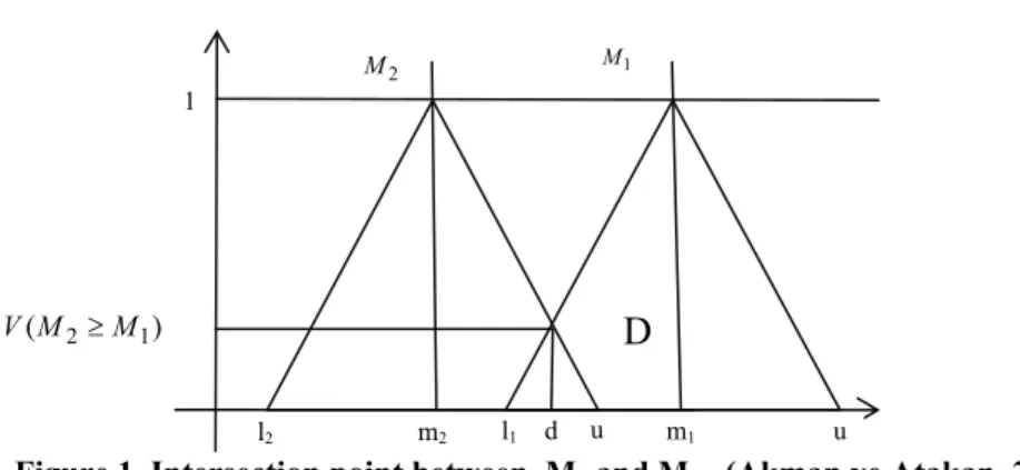
(11)Step 2: Since, M2( ,l m u2 2, )2 and M1( ,l m u1 1, )1 are the two triangular fuzzy numbers, Degree of possibility of M2 M1 is defined as follows;
1 2
2 1
( ) y x|min( M , M ( ) |
V M M sup x y (12)
Equally it can be expressed as in the (13)
2 2 1 2 1 1 2 1 2 1 2 2 2 1 1 1, ( ) ( ) ( ) 0, . ( ) ( ) M m m V M M hgt M M d l u l u other m u m l
(13)Equally V M( 2M1) is d, meaning the ordinate of the D which is the highest
Figure 1. Intersection point between M1 and M2 (Akman ve Atakan, 2006)
To compare M1and M2, values of V M( 2M1) and V M( 1M2) are required.
Step 3: Degree of possibility of a convex fuzzy number being higher then the amount of k convex fuzzy numbers Mi(i=1,2,…,k) is defined as follows:
1
2
1 2 .. , , .., ( ), 1,2, , k k iM M and M M and and
V M M M M V M M minV M M i k (14) If we assume '
( ) i i k d A minV S S (15)then k= 1, 2,…..,n; for k i weight vector can be shown as in (16),
' ' ' ' 1 , , . (2 ) T n W d A d A d A (16) Here; Ai(i 1 , 2 , . . . . ,n)Step 4: Normalized weight vectors is expressed as in (17). Here, W is a number which is not fuzzy.
T1 2 n
W d A , d A ,.. d A (17)
5. An Illustrative Example
5.1 Classical Application of Design Failure Mode Effect Analysis
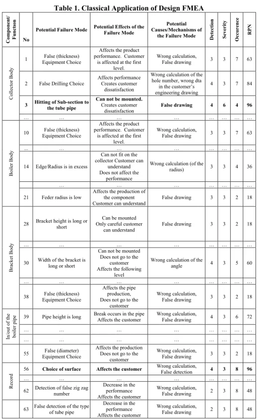
In the first part of the study a classical application of Design FMEA has been included for a company that manufactures heating equipments (radiators) in Turkey. Some of the data can be seen in Table 1.
Risk Priority Numbers (RPN) of the failure modes are calculated in Table 1. Items of 3, 25, 56 and 24 have the highest RPN values. All 63 items are not given in Table 1.
2 M 2 1 ( ) V M M 1 1 M
D
l2 m2 l1 d u m1 uTable 1. Classical Application of Design FMEA
Component/ Funct
ıon
No
Potential Failure Mode Potential Effects of the Failure Mode Causes/Mechanisms of Potential the Failure Mode Detection Severity
Occurence
RPN
Collector Body
1 Equipment Choice False (thickness)
Affects the product performance. Customer
is affected at the first level.
Wrong calculation,
False drawing 3 3 7 63
2 False Drilling Choice Affects performance Creates customer dissatisfaction
Wrong calculation of the hole number, wrong dta
in the customer’s engineering drawing
4 3 7 84
3 Hitting of Sub-section to the tube pipe
Can not be mounted. Creates customer
dissatisfaction False drawing 4 6 4 96
… … … … … … … …
Boiler Bo
dy
10 Equipment Choice False (thickness)
Affects the product performance. Customer
is affected at the first level.
Wrong calculation,
False drawing 3 3 7 63
... … … … … … … …
14 Edge/Radius is in excess
Can not fit on the collector Customer can
understand Does not affect the
performance
Wrong calculation (of the
radius) 3 3 4 36
… … … … … … …
21 Feder radius is low Affects the production of the component
Customer can understand False drawing 3 3 2 18
Brack
et Body
28 Bracket height is long or short Only careful customer Can be mounted can understand
False drawing 3 3 2 18
… … … … … … … …
30 Width of the bracket is long or short
Can not be mounted Does not go to the
customer Affects the following
level
Wrong calculation of the
angle 4 3 5 60
… … … … … … … …
38 Equipment Choice False (thickness)
Affects the pipe production, Does not go to the
customer
Wrong calculation,
False drawing 3 3 2 18
In/out of the boiler pipe
39 Pipe height is long Break occurs in the pipe Affects the customer Wrong calculation, False drawing 4 3 6 72
… … … … … … … …
… … … … … … … …
55 Equipment Choice False (diameter) Affects the production Does not go to the customer
Wrong calculation,
False drawing 3 3 2 18
Record
56 Choice of surface Affects the customer Wrong calculation, False detection 4 3 8 96
… … … … … … … …
62 Detection of false zig zag number Decrease in the performance Affects the customer
Wrong calculation,
False drawing 2 3 8 48
63 False detection of the type of tube pipe Decrease in the performance Affects the customer
Wrong calculation,
5.2. Grey Modeling of Design FMEA
In this section FMEA data in Table 1 is used and the Grey Relational Analysis method under two different assumptions (risk factors have equal and different weights) is applied. The weights of the risk factors are obtained by fuzzy AHP according to expert judgments.
Before explaining Fuzzy AHP methodology, application of Grey Relational Analysis will be explained.
In order to obtain comparative series –which is the first step- , an information series related with the occurrence, detectability and severity of all failure modes in Table 1 are shown in the following matrix.
1 1 1 2 2 2 24 24 24 25 25 25 56 56 56 61 61 61 62 62 62 63 63 63 1 2 3 1 2 3 . . 1 2 3 1 2 3 . 1 2 3 . 1 2 3 1 2 3 1 2 3 X X X X X X X X X X X X X X X X X X X X X X X X 3 3 7 4 3 7 . . 6 3 5 4 3 8 . 4 3 8 . 2 3 5 2 3 8 2 3 8 To reduce the potential risk, the values of all risk factors should be as small as possible. Thus, the standard series is defined as
0( ) 0 1 , 2 ,0 0 3 1,1 1 , X k X X X .
Then, to reveal the degree of fuzzy relation, the difference between values of risk factors and standard series is determined and expressed as the matrix shown below.
01 01 01 02 02 02 024 024 024 025 025 025 056 056 056 061 061 061 062 062 062 062 062 062 1 2 3 1 2 3 . . 1 2 3 1 2 3 . 1 2 3 . 1 2 3 1 2 3 1 2 3 2 2 6 3 2 6 . . 5 2 4 3 2 7 . 3 2 7 . 1 2 4 1 2 7 1 2 7 As previously stated the relational coefficient is calculated with equation 5 which is
0 0 Δ Δ , Δ Δ min max i i max X k X k k . According to the equation, if min1, max7 and =0,5 are used,
0 0 1 0.5 * 7 Δ 0,5 * 7 i i k k is obtained.
01 01 01 02 02 02 024 024 024 025 025 025 056 056 056 061 061 061 062 062 062 062 062 062 1 2 3 1 2 3 . . 1 2 3 1 2 3 . 1 2 3 . 1 2 3 1 2 3 1 2 3 0.82 0.82 0.47 0.69 0.82 0.47 . . 0.53 0.82 0.60 0.69 0.82 0.43 . 0.69 0.82 0.43 . 1.00 0.82 0.60 1.00 0.82 0.43 1.00 0.82 0.43 At the final stage, if all three risk factors is considered to have equal weights, following equation can be applied to determine the degree of relation.
3 01 0 1 1 ( ) 3 i k k k
For example; RPN for first failure mode has been obtained as;
01 1 01 1 01 2 01 3 1 0.82 0.82 0.47 0.7033
3 3
k
In the next section of the study, Risk Priority Numbers will be calculated under the assumption of assigning different weights. Then, all three application models will be compared. Therefore results of the assumption of equal weights are not included here. 5.3 FMEA Application under the Assumption of Assigning Different Weights to Risk Factors with Fuzzy AHP
In order to assign different weights to the risk factors, three quality experts have been asked to compare the importance of the risk factors. In the classical method, the pair wise comparison is made with “nine point scale”.
This discrete scale shows the decision makers’ judgments or priorities among the options such as equally, moderately, strongly, very strongly, or extremely preferred. This scale has the advantages of simplicity and easiness for use, but it doesn’t take into account the uncertainty related with the persons’ judgment to a number (Kwong and Bai, 2002).
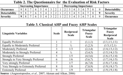
In this study, triangular fuzzy numbers are used to represent pair wise comparisons of risk factors in order to overcome vagueness. The prepared questionnaire, classical and fuzzy AHP scales are shown below in Table 2 and Table 3, respectively.
Table 2. The Questionnaire for the Evaluation of Risk Factors Increasing Importance Decreasing Importance
Occurence 9 8 7 6 5 4 3 2 1 2 3 4 5 6 7 8 9 Detectability Detectability 9 8 7 6 5 4 3 2 1 2 3 4 5 6 7 8 9 Severity Severity 9 8 7 6 5 4 3 2 1 2 3 4 5 6 7 8 9 Occurence
Table 3. Classical AHP and Fuzzy AHP Scales
Linguistic Variables Scale Reciprocal Scale Triangular Fuzzy Scale Triangular Fuzzy Reciprocal Scale Equally Preferred 1 1 (1,1,1) (1/1,1/1,1/1)
Equally to Moderately Preferred 2 ½ (1,2,3) (1/3,1/2,1) Moderately Preferred 3 1/3 (2,3,4) (1/4,1/3,1/2) Moderately to Strongly Preferred 4 ¼ (3,4,5) (1/5,1/4,1/3) Strongly Preferred 5 1/5 (4,5,6) (1/6,1/5,1/4) Strongly to Very Strongly Preferred 6 1/6 (5,6,7) (1/7,1/6,1/5) Very strongly Preferred 7 1/7 (6,7,8) (1/8,1/7,1/6) Very Strongly to Extremely Preferred 8 1/8 (7,8,9) (1/9,1/8,1/7) Extremely Preferred 9 1/9 (8,9,9) (1/9,1/9,1/8) Source: (Angnostopoulos, et al., 2007; Akman and Alkan, 2006)
The evaluation matrices belong to all three Decision Makers (DM) are obtained as follows; 1 1 1 1 7 9 1 7 1 9 9 9 1 O D S O DM D S 2 1 1 1 6 9 1 6 1 9 9 9 1 O D S O DM D S 3 1 1 1 6 9 1 6 1 8 9 8 1 O D S O DM D S
Then, the comprehensive pair wise comparison matrix has been obtained by combining the evaluation scores of the three decision makers with the equation 18.
,
,
1 1
ij k ijk ij k ijk ij k ijk
l min a m b u max c
k
(18)After obtaining the pairwise comparison matrix than can be seen in Table 4, risk factors’ weights have been determined by using fuzzy AHP.
Table 4. Fuzzy Pair wise Comparison Matrix
Occurrence Detectability Severity
Occurence 1 1 1 0.143 3.714 7 0.125 2.442 7
Detectability 0.143 2.464 7 1 1 1 0.125 0.137 0.143
In this study first synthetic values have been calculated according to equation 8. Synthetic extent values of the risk factors are shown below.
1.268;7.156;15 *
1 ; 1 ; 1 (0.032;0.305;1.404) 40.123 23.471 10.679 o S
1.268;3.601;8.143 *
1 ; 1 ; 1 (0.032;0.153;0.762) 40.123 23.471 10.679 D S
8.143;12.714;17 *
1 ; 1 ; 1 (0.203;0.542;1.591) 40.123 23.471 10.679 S S Each risk factors’ degree of possibility has been compared by using the equation 14.
O D
1
O S
0.8351
D S
0.5896V S S V S S V S S
D O
0.53207
S O
1
S D
1V S S V S S V S S
Then risk factors’ priorities are calculated by using equation 9.
' min 1;0.8351 0.8351 O d C
' min 1;1 1 S d C 3 1 '( ) 0.8351 0.53207 1 2.36717i i d C
The risk factors’ weights have been obtained as the following;
0.8351 0.3527 2.36717 O 0.53207 0.2247 2.36717 D 1 0.4224 2.36717 S
During the interview, quality experts stated that if the severity of a failure is too high, there is a risk for human life. Therefore severity was regarded as being more important than occurrence and detectability.
In the next part of the study, fuzzy modeling of Design FMEA has been carried under the assumption of assigning different weights to risk factors. As recalled, all risk factors’ weights were obtained as S0.4224 O 0.3527 D0.2247 by using
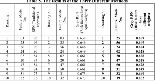
fuzzy AHP. Sum of the weights should be equal to 1. Calculated RPN values based on the three different methods can be seen in Table 5.
Comparing the results in Table 5, it is seen that similar priorities are obtained by both the classical FMEA and the Grey FMEA under the assumption of the risk factors having equal weights. However priorities obtained with the assumption of unequal weights were different than the priorities obtained by the assumption of equal weights.
For example, the third failure mode that is the first in the first two methods is not ranked among top ten in the third method. Another example is that 25th failure mode
is placed first in the last application, whereas it was second in the first two applications. Based on these results, we can say that risk factors with different weights lead to different results in Design FMEA application. If it is accepted that the application of FMEA, under the assumption of different weights overcome the shortcomings of the traditional FMEA, then such a method can be beneficial in identifying and eliminating the most severe failure modes.
Table 5. The Results of the Three Different Methods
Ranking 1 Fail ur e Mode No: RPN (Traditional approach) Ranking 2 Fail ur e Mode No: Grey RPN
(Risk factors have equal weights)
Ranki
ng 3
Failure Mode
No:
Grey RPN (Risk factors
have different wei ghts) 1 03 96 1 03 0.638 1 25 0.609 2 25 96 2 25 0.646 2 56 0.609 3 56 96 3 56 0.646 3 24 0.624 4 24 90 4 24 0.649 4 02 0.628 5 02 84 5 02 0.661 5 20 0.628 6 20 84 6 20 0.661 6 47 0.628 7 47 84 7 47 0.661 7 50 0.628 8 50 84 8 50 0.661 8 31 0.649 9 31 75 9 31 0.673 9 32 0.649 10 32 75 10 32 0.673 10 39 0.652
6. Conclusion
FMEA provides an efficient tool for product design and process planning by detecting the potential product and process failures and by taking actions to prevent them in the early stages. In the traditional FMEA, the failure modes that have to be handled primarily are determined according to the RPN values which are estimated by multiplying values of three different risk factors. However this practice has some drawbacks, such as obtaining same RPNs by multiplying different values of risk factors and taking no account of the weights of the risk factors.
In this study, a different approach to the theory of FMEA which is the Grey Relational Approach was used. The first application of Grey Theory was achieved under the assumption of risk factors having equal weights. In the second one, risk factors were assigned different weights estimated by fuzzy AHP based on quality experts’ evaluations. This is a considerable development in the field of FMEA since assigning different weights using fuzzy AHP is a new approach to FMEA (Hu et al., 2009). In some previous studies about FMEA, there were some generally accepted values for the weights of the risk factors. For example, in the study of Ben Daya ve Raouf (1996) weights of the risk factors were taken as 0.3, 0.4, and 0.3, for occurrence,
detectability and severity respectively. The reason for detectability having the highest weight is the importance of detecting the failure before it reaches to the customer (Ben-Daya and Raouf, 1996). In the present study, in order to estimate the weights of the risk factors, Fuzzy Analytic Hierarchy Method (AHP) was used. Fuzzy AHP was used in the environmental field before (Hu et al., 2009). However this study provides a contribution to the literature by using Fuzzy AHP in FMEA in the manufacturing field. This is an important contribution because FMEA is highly used in the manufacturing field.
In this study, the results of the three applications (classical and the other two) were compared and the differences were interpreted. The obtained results under the assumption of assigning different weights to the risk factors differ from the other two applications. For example, 3rd failure mode that is the first in the first two
applications (classical and grey FMEA with equal weights) is not ranked among top ten in the third application (fuzzy AHP with different weights). 25th failure mode is
placed first in the third application. Due to these results, fuzzy AHP method revealed a difference from the methods with the assumption of equal weights. Thus, with this study a new perspective about prioritization of the failure modes is presented. This new perspective is a contribution to the literature, because it proposes a more efficient model for prioritization of the failure modes. Identifying the most severe failure modes is an important phenomenon for the quality focused firms. Since fuzzy AHP approach to FMEA eliminates previously stated shortcomings of classical approach, it is a useful tool in identifying the failure modes that should be handled primarily. Thus, the limited resources of businesses can be effectively allocated to eliminate the most severe failure modes.
In this study, there is a point that may be considered as a limitation. Quality experts’ judgments, either in calculation of RPN values or assignment of weights to risk factors influence the priority ranking of the failure modes. It must not be forgotten that priority ranking will change if any change happens to the evaluation of decision makers. Thus, replication of this study with different decision makers and observing what kind of changes occur will be another contribution to the literature.
References
AKMAN, G., ATAKAN, A. (2006). Tedarik Zinciri Yönetiminde Bulanık AHP yöntemi kullanılarak tedarikçilerin performansının ölçülmesi: Otomotiv Yan Sanayiinde bir uygulama. İstanbul Ticaret Üniversitesi Fen Bilimleri Dergisi, 5(9), 23-46.ss.
ANGNOSTOPOULOS, K. P., GRATZIOU, M. and VAVATSIKOS, A.P. (2007). Using the Fuzzy Analytical Hierarchy Process for Selecting Wastewater Facilities at Prefecture Level. European Water, 19(20), 15-24. ss.
BAYSAL, M. E., CANIYILMAZ, E. and EREN, T. (2002). Otomotiv Yan Sanayinde Hata Türü ve Etkileri Analizi, Teknoloji. 5(1-2), 83-90. ss.
BEN-DAYA, M. and RAOUF A. (1996). A Revised Failure Mode and Effects Analysis Model, International Journal of Quality and Reliability Management, 13(1), 43-47. ss. BILGIN, Ö. (2006). Hata Türü ve Etkileri Analizinde Bulanık Mantık Uygulaması.
Unpublished Masters. Thesis, KocaeliUniversity, Institute of Physical Sciences
CANBOLAT, R. (2008). Hata Türü ve Etkileri Analizinde Analitik Ağ Süreci ve Bulanık Mantık Uygulaması. Unpublished Masters Thesis. Sakarya University, Institute of Physical Sciences.
CHANG, D.Y. (1996), Applications of the extent analysis method on fuzzy AHP, European Journal ofOperational Research, Vol. 95, 649-55. ss
CHANG, C.L., Liu, P.H., Wei, C.C. (2001). Failure Mode and Effect Analysis Using Grey Theory. Integrated Manufacturing Systems, 12(3), 211-216. ss.
CHANG, K. and Wen, T., (2009). A novel efficient approach for DFMEA combining 2-tuple and the OWA operator. Expert Systems with Applications, 37(3), 2362–2370. ss.
CHIN, K.-S., Chan, A. and Yang, J.-B. (2008), Development of a Fuzzy FMEA Based Product Design System. International Journal of Advance Manufacturing Technology, 36, 633-649. ss.
DENG, H. (1999). Multicriteria analysis with fuzzy pairwise comparison. IEEE Fuzzy Systems Conference Proceedings, Seoul ,South Korea, 726 – 731. ss.
ERGINEL, N. M., (2008). Tasarım Hata türü ve etkileri analizinin etkinliği için bir model ve uygulaması. Endüstri Mühendisliği Dergisi, 15(3), 17-26. ss.
HU, A.H., Hsu, C.W., Kuo, T.C. and Wu, W.C. (2009). Risk evaluation of green components has hazardous substance in using FMEA and FAHP. Expert Systems with Application,s 36(3), 7142-7147. ss.
KAHRAMAN,C., CEBECI, U., ULUKAN, Z. (2003). Multi-criteria supplier selection using fuzzy AHP.Logistics Information Management.16(6),382-394. ss.
KESKIN G. A., ÖZKAN C. (2009). An alternative evaluation of FMEA: Fuzzy Art Algorithm. Quality and Reliability Engineering International, 25, 647–661. ss.
KWONG, C. K., BAI, H. (2002), A Fuzzy AHP Approach to The Determination of Importance Weights of Customer Requirements in Quality Function Deployment. Journal of Intelligent Manufacturing, 13, 367-377. ss.
NARAYANAGOUNDER S., GURUSAMI K. (2009). New Approach for Prioritization of Failure Modes in Design FMEA using ANOVA. WorldAcademy of Science, Engineering and Technology, 49, 524-531. ss.
ÖNDEMIR, Ö., ŞEN G., BARAÇLI H. C.,(2004). Hata Türü ve Etkileri Analizinde Bulanık Mantık Yaklaşımının Kullanılabilirliği. Yöneylem Araştırması/Endüstri Mühendisliği - XXIV Ulusal Kongresi, 15-18 Haziran 2004, içinde Gaziantep – Adana.
PANAGIOTIS, V. P., GIANNIKOS, I. (2009). A fuzzy multicriteria decision-making methodology for selection of human resources in a Greek private bank.Career Development International, 14(4), 372 – 387. ss.
Potential Failure Mode and Effects Analysis FMEA, Overview of FMEA Strategy, Planning and Implementation, Fourth Edition. (2008). Chrysler LLC, Ford Motor Company, General Motors Corporation,USA, 7-66. ss.
SANKAR, N. R., PRABHU, B. S. (2001). Modified Approach For Prioritization Of Failures in a System Failure Mode and Effects Analysis. International Journal of Quality & Reliability Management, 18(3), 324-335. ss.
SHARMA, R. K., KUMAR, D., KUMAR, P. (2005). Systematic Failure Mode Effect Analysis Using Fuzzy Linguistic Modelling. International Journal of Quality &Reliability Management, 22(9), 986-1004. ss.
STONE, R. B., TUMER, I. Y., STOCK, M. E., (2005). Linking product functionality to historic failures to improve failure analysis in design. Research in Engineering Design, 16, 96–108. ss.
SEGISMUNDO A., MIGUEL P. A. C. (2008). Falure Mode and Effect Analysis (FMEA) in the Context of Risk Management in New Product Development. International Journal of Quality &Reliability Management, 25(9), 899-912. ss.
TAY, K. M., LIM, C. P. (2006). Fuzzy FMEA With A Guided Rules Reduction System for Prioritization of Failures. International Journal of Quality&Reliability Management, 23(8), 1047-1066. ss.
TSAI, C. H., CHANG, C. L., CHEN, L. (2003). Applying Grey Relational Analysis to the Vendor Evaluation Model. International Journal of The Computer, The Internet and Management, 11, 45-53. ss.
WANG, Y. M., CHIN, K. S., POON, G. K. K.,YANG, J. B. (2009). Risk evaluation in failure mode and effects analysis using fuzzy weighted geometric mean. Expert Systems with Applications, 36, 1195–1207. ss.