SCADA üzerinden bir adaptif kontrol uygulaması

AN ADAPTIVE CONTROL APPLICATION USING SCADA Ceylan TÜRKER

Master of Science Thesis Mechatronics Engineering Yrd. Doç. Dr. Murat TÜRE

i

T.C.

BURSA TEKNİK ÜNİVERSİTESİ

FEN BİLİMLERİ ENSTİTÜSÜ

SCADA ÜZERİNDEN BİR ADAPTİF KONTROL

UYGULAMASI

YÜKSEK LİSANS TEZİ

Ceylan TÜRKER

Mekatronik Anabilim Dalı

BURSA Ocak 2016

ii

T.C.

BURSA TEKNİK ÜNİVERSİTESİ

FEN BİLİMLERİ ENSTİTÜSÜ

AN ADAPTIVE CONTROL APPLICATION USING

SCADA

A THESIS FOR THE DEGREE OF MASTER OF

SCIENCE

Ceylan TÜRKER

BURSA January 2016

iii

YÜKSEK LİSANS TEZİ ONAY FORMU

CEYLAN TÜRKER tarafından Yard. Doç. Dr. MURAT TÜRE yönetiminde hazırlanan SCADA ÜZERİNDEN BİR ADAPTİF KONTROL UYGULAMASI başlıklı tez, kapsamı ve niteliği açısından incelenmiş ve Yüksek Lisans Tezi olarak kabul edilmiştir.

Sınav Jüri Üyeleri

Yrd. Doç. Dr. Murat TÜRE

(Doğa Bilimleri, Mimarlık ve Mühendislik Fakültesi, Mekatronik Mühendisliği) Doç. Dr. Ali Rıza YILDIZ

(Doğa Bilimleri, Mimarlık ve Mühendislik Fakültesi, Makina Mühendisliği) Yrd. Doç. Dr. Hüseyin LEKESİZ (Doğa Bilimleri, Mümarlık ve Mühendislik Fakültesi, Makina Mühendisliği)

Tez Savunma Tarihi: 04/01/2016

Fen Bilimleri Enstitüsü Müdürü

iv

İNTİHAL BEYANI

Bu tezde görsel, işitsel ve yazılı biçimde sunulan tüm bilgi ve sonuçların akademik ve etik kurallara uyularak tarafımdan elde edildiğini, tez içinde yer alan ancak bu çalışmaya özgü olmayan tüm sonuç ve bilgileri tezde kaynak göstererek belgelediğimi, aksinin ortaya çıkması durumunda her türlü yasal sonucu kabul ettiğimi beyan ederim.

v TEŞEKKÜR

Yüksek lisans eğitimim boyunca bilgi ve tecrübelerinden yararlandığım, tez süresi boyunca laboratuvar çalışmaları için imkan sağlayan, ayrıca bilgilerini paylaşırken göstermiş olduğu hoşgörü ve sabırdan dolayı değerli hocam, sayın Yrd. Doç. Dr. Murat TÜRE' ye,

Çalışma boyunca sorularımı cevaplayıp, deneyimleriyle bana yol gösteren Elekt. Elektronik Müh. Onur Atasoy' a ve

Eğitim hayatım boyunca desteklerini esirgemeyen değerli iki insan annem ve babama teşekkürlerimi sunarım.

vi CONTENTS

page number

Outer Cover

Inner Cover i

Tez Onay Formu iii

İntihal Beyanı iv Teşekkür v Contents vi Figures ix Abbreviations xi Özet xii Abstract xiii 1. INTRODUCTION 1 2. ADAPTIVE CONTROL 1

2.1 Direct and Indirect Adaptive Control 2

2.2 Robust Control 3

2.3 Self-oscillating Adaptive System 4

2.4 Self-tuning Regulators 5

2.5 Gain Scheduling 5

2.6 Model Reference Adaptive Control (MRAC) 7

2.6.1. MIT and Lyapunov Rules 8

3. DC MOTOR CONTROL USING MODEL REFERENCE BASED ADAPTIVE CONTROLLER 10

3.1 The PID Controller 11

3.1.1 Modeling the System with Equations 11

3.1.2 Building a Block Diagram Model of the System 12

3.2 Model Reference Adaptive Control System 14

3.3 Reference Model 17

3.4 Plant Model 18

3.5 Adaptive Controller 19

3.5.1 Purposed Controller 19

3.5.2 Adaptive Mechanism 20

vii

page number

4.1 SCADA Interface 24

4.2 Siemens SIMATIC S7-200 PLC 25

5. COMMUNICATION IN THE SYSTEM 26

5.1 S7-200 Network Communication 26

5.2 Setting the Baud Rate and Network Address 26

5.3 Profibus 28

5.4 Configuring the OPC Server with S7-200 PC Access 29

5.5 WinCC Flexible 31

6. UNLOADING AND CARRYING STATION 32

6.1 Components Used in the System 33

6.1.1 Limit Switch 33

6.1.2 Manometer and Dryer Module 33

6.1.3 Selenoid Valve Group 34

4.1.4 Unloading Unit 35

4.1.5 Vacuum Generator 36

4.1.6 Vacuum Switch 37

4.1.7 Carrying Unit 37

7. PROCESSING STATION 38

7.1. Components Used in the System 39

7.1.1 Optical Sensor 39

7.1.2 Inductive Sensor 40

7.1.3 Rotary Table 41

7.1.4 Processing Unit 42

7.1.5 Carrying Unit 43

8. TEST AND SEPERATION STATION 43

8.1. Components Used in the System 44

8.1.1 Siemens TD-200 Operator Panel 44

8.1.2 Optical Sensor 45

8.1.3 Optical Contrast Sensor 45

9. RESULTS 45

viii

page number

APPENDIX

APPENDIX 1. SCADA SCREENS AND NOTICES 51 APPENDIX 2. PLC PROGRAMS 53

ix FIGURES

page number

Figure 2.1 General Feedback system 4

Figure 2.2 Basic Block Diagram of a Gain Scheduling System 6

Figure 2.3 Basic Block Diagram of a Model Reference Adaptive System 7

Figure 3.1 PID Controller 11

Figure 3.2 PI Controller in Simulink 13

Figure 3.3 First Simulink Model 14

Figure 3.4 Generator Pulse Wave 14

Figure 3.5 Block Diagram of Model Reference Adaptive System 15

Figure 3.6 DC Motor Output and Comparison with reference Model 16

Figure 3.7 DC Motor Output and Comparison with reference Model 16

Figure 3.8 DC Motor Output and Comparison with reference Model 16

Figure 3.9 Simulink Model 17

Figure 3.10 Bode Diagram of Proposed reference Transfer Function 18

Figure 3.11 Plant Model 19

Figure 3.12 Purposed Controller in Simulink 19

Figure 3.13 Adaptive Mechanism 20

Figure 3.14 Output DC Motor and Comparison with Reference 21

Figure 3.15 Input of the Proposed Adaptive Control Model 22

Figure 3.16 Input in Simulink 22

Figure 3.17 Closed-loop DC Motor Control System 23

Figure 4.1 Components and General Structure of the Designed System 23

Figure 4.2 Main SCADA Screen 24

Figure 4.3 S7-200 Working Principle 25

Figure 5.1 STEP 7-Micro/WIN Communication Block 27

Figure 5.2 STEP 7-Micro/WIN Communication Ports 28

Figure 5.3 Profibus Cable 28

Figure 5.4 Profibus Cable Connections 29

Figure 5.5 OPC Server Relations 29

Figure 5.6 Adding New PLC to PC Access 30

Figure 5.7 PC Access Communication Settings 30

x

page number

Figure 5.9 WinCC Flexible 2008 Communication 31

Figure 6.1 Unloading and Carriying Station 32

Figure 6.2 Manometer and Dryer Module 34

Figure 6.3 Unloading Unit 35

Figure 6.4 Cross-section of Vacuum Generator 36

Figure 6.5 Vacuum Process 36

Figure 6.6 Vacuum Switch 37

Figure 6.7 Carrying Unit 38

Figure 7.1 Processing Station 39

Figure 7.2 Optical Sensor Working Principle 40

Figure 7.3 Electirical Wiring Diagram of the Optical Sensor 40

Figure 7.4 Inductive Sensor Working Principle 41

Figure 7.5 Electirical Wiring Diagram of the Inductive Sensor 41

Figure 7.6 Rotary Table 42

Figure 7.7 Processing Unit 42

Figure 8.1 Test and Seperation Station 44

xi ABBRIVIATIONS

CPU Central Processing Unit DC Direct Current

HMI Human Machine Interface LED Light Emitting Diod

MIT Massachusetts Institute of Technology MRAC Model Reference Adaptive Control MRAS Model Reference Adaptive System OLE Object Linking and Embedding OPC OLE for Process Control PC Personal Computer

PLC Programmable Logic Controller

SCADA Supervisory Control and Data Acquisition STC Self-tuning Controller

xii ÖZET

SCADA ÜZERİNDEN BİR ADAPTİF KONTROL UYGULAMASI

Ceylan TÜRKER

Bursa Teknik Üniversitesi Fen Bilmleri Enstitüsü

Mekatronik Mühendisliği Anabilim Dalı Yüksek Lisans Tezi

Yrd. Doç. Dr. Murat TÜRE 04.01.2016, 55

Bu tez çalışmasında, adaptif kontrol çeşitleri incelenmiş ve bant hız kontrolü sağlanmıştır. Matlab üzerinden bir motorun konum kontrolü adaptif şekilde modellenmiştir. Üç adet istasyona ait otomasyon sistemi için bir SCADA yazılım arayüzünün WinCC Flexible nesne tabanlı programlama yazılımı ile tasarımı ve kontrolü, sistem elemanları ile birlikte ayrıntılı olarak anlatılmıştır.

Bu sistem, boşaltım ve taşıma, işleme, test ve ayırma olmak üzere üç istasyondan oluşmaktadır. Bilgisayar ile sistem arasındaki veri alışverişi, seri haberleşme portu üzerinden PLC ile sağlanmaktadır. Sistemin ana PLC yazılımına göre tasarlanan SCADA arayüzünde, işlem yapılan malzemenin istasyonlardaki durumları gerçek zamanlı olarak gösterilmektedir.

xiii ABSTRACT

AN ADAPTIVE CONTROL APPLICATION USING SCADA

Ceylan TÜRKER

Bursa Technical University

Graduate School of Natural and Applied Science Mechatronics Engineering

Master of Science Thesis Assist. Prof. Dr. Murat TÜRE

04.01.2016, 55

In this study, adaptive control types are studied and speed control of the band is achieved. Position control of a motor is modeled in adaptive way by using Matlab. Designing and controlling of a SCADA software interface for an automation system belonging to three different stations are described in detail by using WinCC Flexible object oriented programming software.

This system is composed of three stations of unloading and carrying, processing, test and separation. Data transferring between the computer and the system was carried out by PLC (Programmable Logic Controller) via serial communication port. On the designed SCADA interface, conditions of processing material at the stations are shown at real time according to basic PLC program.

1 1. INTRODUCTION

In operate and control of the systems, accurately and quickly reaching of the available data and information to the required centers are important. It is possible with the application of the real-time controlling and monitoring systems. Furthermore, continuous monitoring and control of the system as a whole from a single center can only be done with real-time supervisory control and data acquisition (SCADA) systems. In order to meet these objectives, there are packages SCADA software for simple systems.

In this study, firstly an adaptive controller for a dc motor is examined in two similar ways and simulated, secondly an application of monitoring, controlling and running the desired adaptive algorithms to control more than one system with a single SCADA interface is shown. Necessary communication methods are also given in detail for controlling and monitoring of multiple systems through a single interface. Object-oriented programming software is used for SCADA interface. As the monitored system three station of the university's mechatronics laboratory are chosen, monitoring and controlling of the station are provided from a single center.

2. ADAPTIVE CONTROL

In everyday language, to adapt means to change a behavior to conform to new circumstances. Intuitively, an adaptive regulator is a regulator that can modify its behavior in response to changes in the dynamics of the process and the disturbances [1]. Different adaptive control types are classified according to their adaptation mechanism and form, chosen behavior criteria and adjusted parametres. The cases which adaptive control need to be used can be sorted as changes in equipment features, work and environment conditions, expected product features. These changes can be detect by sensors that controls the process parametres [2]. If the system in this study is considered, the function of the adaptive control is to provide suitable working conditions for the product.

In the early 1950s there was extensive research on adaptive control, in connection with the design of autopilots for high performance aircraft. The early

2

experiments, which used analog implementations, were plagued by hardware problems. A great number of industrial control loops are today under adaptive control. These include a wide range of applications in aerospace, process control, ship steeringi robotics and others industrial control systems [1].

We say the design of control algorithms for a class of plant models described by the liear differential function.

𝑥̇ = 𝐴𝑥 + 𝐵𝑢, 𝑥(0) = 𝑥₀

𝑦 = 𝐶𝑇_{𝑥 + 𝐷𝑢 (2.1)}

In (2.1) x ∈ Rn _{is the state of the model, u ∈ R}r _{the plant input, and y ∈ R}l

the plant model output. The matrices A ∈ Rnxn_{, B ∈ R}nxr_{, C ∈ R}nxl _{and D ∈ R}lxr

could be constant or time varying. This class of plant models is quite general because it can serve as an approximation of nonlinear plants around operating points. For an operating point i, where Ai, Bi, Ci ve Di are functions of that operating point. As the

operating point changes leading to different values for Ai, Bi, Ci ve Di. Because the

output response y(t) carries information about the x as well as the parameters [3].

Adaptive systems are inherently nonlinear. Their behavior is therefore quite complex, which makes them difficult to analyze. Progress in theory has been slow, and much work remains before a reasonably complete, coherent theory is available. Because of the complex behavior of adaptive systems, it is necessary to consider them from several points of view. Theories of nonlinear systems, stability, system identification, recursive parameter estimation, optimal control and stochastic control all contribute towards the understanding of adaptive systems. Many adaptive algorithms are based on the assumption that parameters change more slowly than the state variables of the system. The rate of change of the parameters can be controlled by the designer's choice of the adaptation rate [1].

2.1. Direct and Indirect Adaptive Control

Consider the basic philosophy for designing a controller, one of the key points is the specification of the desired control loop performance. In many cases, the desired performance of the feedback control system can be specified in terms of the characteristics of a dynamic system which is a realization of the desired behavior of

3

the closed loop system. For example, a tracking objective specified in terms of risetime, and overshoot, for a step change command can be alternatively expressed as the input-output behavior of a transfer function (for example a second order with a certain resonance frequency and certain damping). A regulation objective in a deterministic environment can be specified in terms of the evolution of the output starting from an initial disturbed value by specifying the desired location of the closed loop poles. In these cases, the controller is designed such that for a given plant model, the closed loop system has the characteristics of the desired dynamic system [4]. In the direct algorithm the controller parameters are updated directly.

In the indirect control the basic idea is that a suitable controller can be designed online if a model of the plant is estimated online from the available input-output measurements. The scheme is termed indirect because the adaptation of the controller parameters is done in two stages. First is online estimation of the plant parameters and the second is online computation of the controller parameters based on the current estimated plant model. The indirect adaptive control scheme offers a large variety of combinations of control laws and parameter estimation techniques. To better understand how these indirect adaptive control works, it is useful to consider in more detail the online estimation of the plant model [4].

If these two classes of controls are discussed: indirect and direct algorithms. The indirect algorithms are a straightforward implementation in which process parameters are estimated and controller parameters are computed by using some design equations. In the direct algorithms the controller parameters are estimated directly [1].

2.2. Robust Control

The ultimate goal of any control design is to meet the performance requirements when implemented on the actual plant. In order to meet such a goal, the controller has to be designed to be insensitive, i.e., robust with respect to the class of plant uncertainties that are likely to be encountered in real life. In other words, the robust controller should guarantee closed loop stability and acceptable performance not only for the nominal plant model but also for a family of plants, which most likely, include the actual plant.

4

Let us consider the feedback system of Figure 2.1 where C, F are designed to stabilize the nominal part of the plant model whose transfer function is G0(s). The

transfer function of the actual plant is G(s) and du, d, dn, ym are external bounded

inputs. The difference between G(s) ve G0(s) is the plant uncertainty. Thus G(s) may

represent a family of plants with the same nominal transfer function G0(s) and plant

uncertainty characterized by some upper bound in the frequency domain. We say that the controller (C, F) is robust with respect to the plant uncertainties in G(s) if, in addition to G0(s), it also stabilizes G(s). The property of C, F to stabilize G(s) is

referred to as robust stability [3].

The robust design method will generally give systems that respond faster when the parameters change, but it is important that the range of parameter variation be known. The adaptive regulator responds more slowly but can generally handle larger parameter variations [1].

2.3. Self-oscillating Adaptive System

An interesting approach for compensation of variations in the process gain was used in an autopilot proposed by Honeywell. The self-oscillating adaptive system has the same structure as the high-gain system. The basic idea is to have a feedback loop whose gain is as high as possible combined with a feedforward compensation to give the desired response to command signals. The high loop gain is maintained by introducing a relay in the feedback loop. This will create a limit cycle oscillation. Thus system with relay feedback automatically adjusts itself to give a reasonable amplitude margin [5].

5 2.4. Self-tuning Regulators

For the two approaches, one is the design of an adaptive controller did not require detailed knowledge of the dynamic behaviour of the controlled system. Another approach to adaptive control is based on the recursive estimation of the characteristics of the system and disturbancez ans updating the estimates, so monitoring possible changes. Using this knowledge appropriate methods can be employed to design the optimal controller. This kind of controller, which identifies unknown processes and then synthesizes control (adaptive control with recursive identification) is referred to in the literature as self-tuning controller (STC) [6].

2.5. Gain Scheduling

Adaptive control is not the solution to all control problems. It is therefore appropriate to include a discussioon of alternatives to adaptive control. A special kind of open loop adaptation or change of regulator parameters can be discussed. In many situations it is known how the dynamics of a process change with the operating conditions of the process. One source for the change in dynamics may be nonlinearities that are known. It is then possible to change the parameters of the controller by monitoring the operating conditions of the process. This idea is called gain scheduling since the scheme was originally used to accomodate changes in process gain only [1].

Let us consider a model where for each operating point i (i= 1, 2,..., N), the parameters Ai, Bi, Ci ve Di are known. For a given operating point i, a feedback

controller with constant gains, say θi, can be designed to meet the performance

requirements for the corresponding linear model. This leads to a controller, say C(θ), with a set of gains (θ1, θ2, θi,...θN) covering N operating points. Once operating point,

say i, is detected the controller gains can be change to the appropriate value of θi

obtained from the precomputed gain set. Transitions between different operating points that lead to significant parameter changes may be handled by interpolation or by increasing the number of operating points. The two elements that are essential in implementing this approach is a look-up table to store the values of θi and the plant

6

auxiliary measurements that correlate well with changes in the operating points. The approach is called gain scheduling [3].

This is an open loop adaptive control system because the modifications of the system performance resulting from the change in controller parameters are not measured and feedback to a comparison-decision block in order to check the efficiency of the parameter adaptation. The system can fail if for some reason or another the rigid relationship between the environment measurements and plant model parameters changes [4].

In some systems there are auxiliary variables that well to the characteristics of the process dynamics. If these variables can be measured, they can be used to change the regulator parameters. This approach is called gain scheduling because the scheme was originally used to accommodate changes in process gain [1].

The advantage of gain scheduling is that the controller gains can be changes as quickly as the auxiliary measurements respond to parameter changes. However, frequent and rapid changes of the controller gain, may leads to instability. One of the disadvantages of gain scheduling is that the adjustment mechanism of the controller gain is precomputed offline and therefore provides no feedback to compensate for incorrect schedules. Unpredictable changes in the plant dynamics may lead to deterioration of performance. Despite its limitations, gain scheduling is a popular method for handling parameter variations in systems [3].

7

2.6. Model Reference Adaptive Control (MRAC)

Model reference adaptive systems design is theoretically well elaborated and widely disscused in scientific literature. MRAC is one of the main approaches to adaptive control [1, 3]. It was originally proposed by Whitaker at MIT to solve a problem in which the specifications are given in terms of a reference model that tells how the process outputnideally should respond to the command signal [5].

According the basic block diagram of the MRAS, the reference model gives requested response ym or requested state vector xm to reference input signal ur (Figure

2.3).

This approach is based on observation of the difference between the output of the adjustable system ys and the output of the reference model ym. The aim of the

adaptation is convergence of the static and dynamic characteristics of the adjustable system, i.e., the closed loop, to the characteristics of the reference model. This, in fact, is an adaptive system with forced behaviour where the comparison between this forced behaviour and the behaviour (response) of the adjustable system ys (control

loop), provides the error ε. The task of the appropriate control mechanism is to reduce error ε or errors in the state vector x between the reference model and the adjustable system to a minimum for the given criteria. This is done either by

8

adjusting the parameters of the adjustable system or by generating a suitable input signal (Figure 2.3). The dual character of this adaptive system is important since it can be used both for control and to identify the parameters of the model process or estimate the state of the system [6].

2.6.1. MIT and Lyapunov Rules

Adaptive control techniques allow to control systems where certain system parameters are not known or change ove time i.e. due to changing operating environment. The following example deals with a first order system with one unknown parameter, the system gain value b. The second parameter, the time constant a, is assumed to be known. For the plant process with unknown parameters, a specific control law alters the reference input signal in order for the plant’s output signal to match the reference model. This control law usually features time-variant controller parameter θ which reflect the algorithm’s adaptation to the given plant system [7].

The reference model,

𝑌𝑚(𝑠) = 𝐺𝑚(𝑠)𝑅𝑚(𝑠) =_𝑠+𝑎𝑏𝑚 𝑅(𝑠) (2.2)

produces a model output ym and from the process,

𝑌_𝑝(𝑠) = 𝐺_𝑝(𝑠)𝑈(𝑠) = _𝑠+𝑎𝑏 𝑈(𝑠) (2.3)

yp results. Taking the difference of these two signals yields the tracking error e. In

order to ensure that process dynamics,

𝑦_𝑝̇ + 𝑎𝑦̇ = 𝑏𝑢 (2.4) _𝑝 match the desired reference dynamics,

𝑦𝑚̇ + 𝑎𝑦𝑚̇ = 𝑏𝑢 (2.5)

𝑢 = 𝑟𝜃 (2.6) the control law is an intuitive choice. Indeed, if the gain value θ is set to, θ = bm / b,

then (2.4) becomes (2.5).

MIT rule is a common used rule. This adaptation mechanism is defined by, _𝑑𝑡𝑑 𝜃 = −𝛼𝑒𝑦_𝑚 (2.7)

9

and incorporates the output error e as well as the reference model’s output ym. gibi

çıkış hatasını da kapsar. To derive this update law, a cost function is defined first: 𝐽 =1₂𝑒2 _(2.8)

Essentially, the parameter θ is set to follow the “steepest descent” i. e. move along the negative gradient with a certain adaptation gain α.

𝑑

𝑑𝑡𝜃 = −𝛼 𝑑

𝑑𝜃𝐽

= −𝛼𝑒_𝑑𝜃𝑑 𝑒(𝜃) (2.9) In order to calculate the sensitivity derivative 𝑑

𝑑𝑡𝑒(𝜃) the system equations of model

and plant process are inserted.

_𝑑𝑡𝑑 𝜃 = −𝛼_𝑑𝜃𝑑 (𝑦_𝑝− 𝑦_𝑚) = −𝛼𝑒_𝑑𝜃𝑑 (ℒ−1_{𝐺 𝑝(𝑠)𝑈(𝑠) − 𝐺𝑚(𝑠)𝑅(𝑠)}) = −𝛼𝑒_𝑑𝜃𝑑 ((ℒ−1_{𝐺 𝑝(𝑠)𝜃𝑅(𝑠) − 𝐺𝑚(𝑠)𝑅(𝑠)}) = −𝛼𝑒_𝑑𝜃𝑑 (ℒ−1_{𝑏𝐺 𝑚(𝑠)𝜃𝑅(𝑠) − 𝐺𝑚(𝑠)𝑅(𝑠)}) = −𝛼𝑒𝑏ℒ−1_{𝐺 𝑚(𝑠)𝑅(𝑠)} = −𝛼𝑒𝑏𝑦𝑚 (2.10)

Finally merging α and b to a single gain value γ = α b yields the update law. _𝑑𝑡𝑑 𝜃 = −𝛾𝑒 𝑏𝑚

𝑠+𝑎𝑟

= −𝛾𝑒𝑦𝑚 (2.11)

A second option for an update law is the Lyapunov rule,

_𝑑𝑡𝑑 𝜃 = −𝛾𝑒𝑟 (2.12) where r is the reference input signal for both systems. In order to derive this formula, the following Lyapunov function is defined [1].

𝑉 =1₂𝛾𝑒2₊1 2𝑏 (𝜃 − 𝑏𝑚 𝑏) 2 (2.13) The time derivative of V can be found as,

𝑉̇ = 𝛾𝑒𝑒̇ + 𝑏𝜃̇ (𝜃 −𝑏𝑚 𝑏)

2

(2.14) and its negative definiteness would guarantee the tracking error going to zero along the system’s trajectories. Inserting the dynamic equations of model and plant process,

10 𝑦_𝑝̇ = −𝑦_𝑝+ 𝜃𝑏𝑟 (2.15) 𝑦𝑚̇ = −𝑦𝑚+ 𝑏𝑚𝑟 (2.16) yields 𝑉̇ = 𝛾𝑒(𝑦_𝑝̇ − 𝑦_𝑚̇ ) + 𝑏𝜃̇ (𝜃 −𝑏𝑚 𝑏 ) = 𝛾𝑒(−𝑦_𝑝+ 𝜃𝑏𝑟 + 𝑦_𝑚+ 𝑏_𝑚𝑟) + 𝜃̇(𝑏𝜃 − 𝑏_𝑚) = 𝛾𝑒(−(𝑦𝑝− 𝑦𝑚) + 𝑟(𝜃𝑏 − 𝑏𝑚)) + 𝜃̇(𝑏𝜃 − 𝑏𝑚) = 𝛾𝑒2_{+ (𝛾𝑒𝑟 + 𝜃̇)(𝑏𝜃 − 𝑏} 𝑚) (2.17)

The last line gives the following condition for the Lyapunov function's derivative to be negative definite and thus the update law (2.11).

This result is similar to the MIT rule in equation (2.11), with the only difference being an additional filter operation of r with the reference model dynamics. In both cases, the update law for the parameter θ is defined by its derivative _𝑑𝑡𝑑 𝜃. tarafından tanımlanmıştır. This derivative is the product of a adaptation gain factor -γ and two of the system's signal. Regarding the MIT rule, these two factors are the error signal e ve and the reference model’s output ym. This

relationship is derived using a cost function J(e) and varying the parameter in the direction of the negative gradient. In contrast, the Lyapunov rule is established using the approach of a Lyapunov function whose negative definiteness should be maintained by a suitable update law. This results in the update law being the product of the adaptation gain -γ, the error signal e and the reference input signal r. Therefore, the signal ym as found in the MIT rule, is exchangeed with r in the

otherwise identical Lyapunov adaptation mechanism [7].

3. DC MOTOR CONTROL USING MODEL REFERENCE BASED ADAPTIVE CONTROLLER

In this thesis a DC motor control using model reference based adaptive controller is implemented. The implementation of this system has three steps. The first step is designing the reference model and second step is modelling the plant. For plant model DC motor is used. Final step is designing the adaptive controller.

11 3.1. The PID Controller

This controller replaces the amplifier in the forward path of our closed-loop control system. One example of PID controller is shown in Figure 3.1. "The Plant" just means the equipment whose output is being controlled.

In this figure r is the reference input. Telling the system that we want the output y to settle at a value which will make the transducer output equal to y. e is the error. u is the controller output or controller action. y is the plant output.

Our studies of such systems have began by just using an amplifier instead of the PID controller. The PID controller (also called a Three-Term Controller) actually incorporates what is effectively an amplifier. The output u of the PID controller is:















dt

de

D

edt

I

e

P

u

where P, I and D are the Proportional, Integral and Derivative gains respectively. If I and D are both zero, the controller is just an amplifier with a gain P.

3.1.1. Modeling the System with Equations

A discrete PI controller based on the following equation:

y(k) y_p(k)y_i(k) (3.2) where

12 1 ) ( 1 ) ( ) 1 ( ) ( ) ( ) (        k y k e T K k y k y k e K k y i s i i i p p (3.3)

y(k) — Controller output

e(k) — Error (difference between desired output and actual output) Ts — Sample time

Kp — Proportional gain Ki — Integral gain

The Backward Euler method (a numerical integration approximation) is used to solve the integrator equation from above. This is why the integrator equation goes from yi(k-1) to yi(k).

The output of the integrator equation must fall between -1 and 1. This range is required as an antiwindup measure, or to prevent windup in the system. Windup refers to the condition when the controller is ineffective at reducing the system error, and so the integral state (yi(k)) becomes very large.

3.1.2. Building a Block Diagram Model of the System

To build a block diagram model of the system,

1. Use a step function as the system input (e(k)).

2. Build the integrator equation using the method discussed earlier in this homework.

3. Limit the output of the yi integration to fall within the limits defined below.

4. Define an initial condition of 0 for yi (this can be done by setting an initial

condition in the Unit Delay block).

5. View both the input and output on the same scope. 6. Use variable names to define block parameters. 7. Label the signals and annotate the diagram.

13

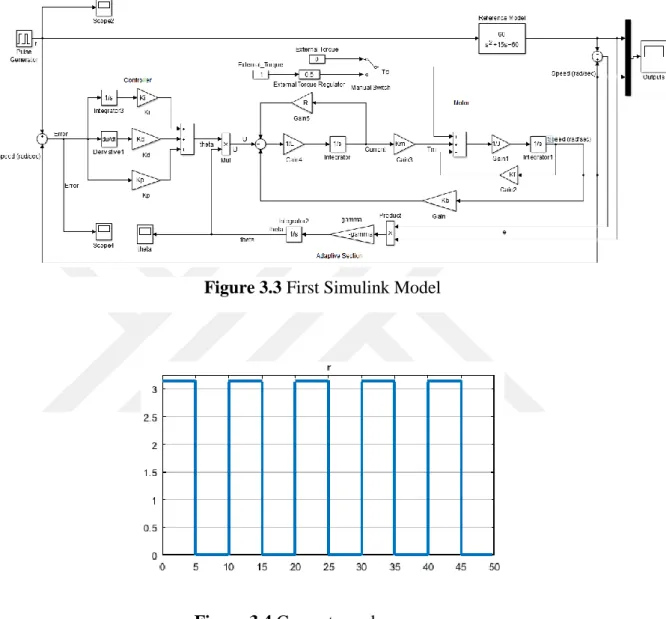
In this project firstly a PID controller is tried for controlling of DC motor. In source the pulse generator with 3 volt amplitude and 100 second period is used. The pulse width of this generator is 50.

The output of continues PID controller is the sum of three individual controller outputs — proportional, integral, and derivative controls:

y(k) y_p(k)y_i(k) y_d(k) (3.4) where





The parameters used in this project is as below.

Table 3.1 Parameters Parameter Ki Kd Kp R L Description Integrator Coefficient Derivative Coefficient Proportional Coefficient Ohms Henrys Value 100 0.1 30 2 0.5 Parameter Km Kb B J Kc

Description torque constant emf constant Nms kg.m2

Value 0.015 0.015 0.2 0.02 1

14

For PID controller 5.28 for Ki and 1.32 for Kd is used, also for Kp 5.28 is

selected. These values is acquired experimentally. The Simulink model that used in the project is shown in Figure 3.3. The input generated signal for this type of simulink is illustrated in Figure 3.4.

3.2. Model Reference Adaptive Control System

The model reference adaptive control system is an important adaptive controller. It may be regarded as an adaptive system in which the desired performance is expressed in terms of a reference model, which gives the desired response to an input signal. This is a convenient way to give specifications for a problem. A block diagram of the model reference adaptive control system is shown

Figure 3.3 First Simulink Model

15

in Figure 3.5. Where the system has an ordinary feedback loop, which is composed of the process and the controller, and another feedback loop that changes the controller parameters. The parameters are changed on the basis of feedback from error em(t), which is the difference between the output of the system y(t) and the

output of the reference model ym(t). The ordinary feedback loop is called the inner

loop, and the parameter adjustment loop is called the outer loop. The mechanism for adjusting the parameters in a model reference adaptive control system can be obtained in two ways: by using a gradient method or by applying Lyapunov stability theory [1].

Adaptive gain  will be chosen by trial and error using simulations in order to achieve a good rate of convergence. Simulation results for the rotor angular position are shown in Figures 5, 6 and 7 for adaptive gains 0.001,0.01,0.1 respectively. All the figures indicate satisfactory convergence of the plant output to that of the model. But the use of a larger value of the adaptive gain  led to a faster convergence of plant output to models. The biggest adaptive gain is chosen as

1 . 0



 because adaptive laws become stiff and difficult to solve numerically on the computer and simulink gives application error for  0.1. The red lines show model output, blue lines show plant output, cyan lines if exist show error signal in all simulations.

16

Figure 3.6 DC Motor Output and Comparison with Reference Model for  0.1

Figure 3.7 DC Motor Output and Comparison with Reference Model for  0.001

17

Objective of this part of the study is to demonstrate how to design and model adaptive controller, tune and analyses its performance using Simulink. Here we have used direct adaptive method called Model Reference Adaptive Controller (MRAC). There are three main elements of this model: Reference Model, Plant Model and Adaptive Controller. The final Simulink model used in this study is shown in Figure 3.9.

3.3. Reference Model

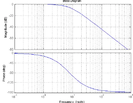
This section of controller models the preferred treatment of closed-loop system. In this thesis, a transfer function for reference model is used. This transfer function is, 60 15 60 ) ( ₂    s s s T (3.6)

This part of the controller captures\models the desired behavior of closed-loop system. In other words, how you like your overall system to behave for a given input is modelled in this subsystem. In this project, reference behavior is modelled as a transfer function. This can also come from closed-loop system specifications

18

described in below figure as desired Rise Time (0.413sec), Settling Time (0.706sec) and Steady State Error (0). Reference Model output, Ym is desired reference

trajectory which Plant output (Yp) has to follow.

In this transfer function lowpass filter is used and the frequency responce of this filter is as Figure 3.10.

3.4. Plant Model

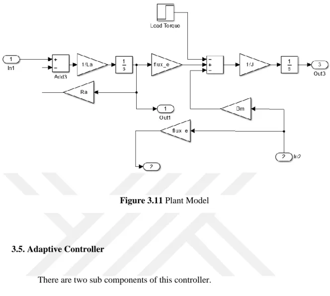
In this study, plant is a DC Motor. One of the many motor parameters, Kf – Mechanical Damping, is considered to be varying. Initial value is assumed to be 0.2. And PID controller is tuned to achieve desired response with this initial value of Kf. Now as motor goes through aging and impact of other environmental conditions, Kf changes, this will change motor behavior. Plant output is Yp. Hence controller has to adapt\change its parameter values to achieve desired response (Yp – Ym = error (e) =

0). This is illustrated in Figure 3.11.

19 3.5. Adaptive Controller

There are two sub components of this controller.

3.5.1. Purposed Controller

Figure 3.11 Plant Model

20

This part of controller is fixed and gains have been tuned for keeping initial plant condition in mind and to achieve overall stability. Output of PI controller is Uc.

3.5.2. Adaptive Mechanism

The goal of this part of controller is to change its output (theta) based on error (e) between plant output (Yp) and reference model output (Ym). How fast it can adapt

(or change its output) depends on parameter called learning rate, gamma. Higher the value of gamma, faster it can adapt to any changes in plant. But there are some side effects also. Controller output (U) is calculated by: U = Uc * theta. Adaptive mechanism is illustrated in Figure 3.13.

By running this model with default values of plant, PI controller and learning rate, it can be observed that overall all closed-loop system is behaving as per reference model. Look at the small difference between blue colored curve and red colored curve. This small error is due to well-tuned PI controller for known plant values (Kf and others). The result is shown in Figure 3.14.

21

In the second part of this study it is illustrated that the position control of the DC motor can be controlled and sustained at specified performance characteristics by using proposed method. The gradient method gives acceptable response but does not guarantee the stability of the system [26]. Whereas proposed method can be used to design the adaptation mechanism satisfy the desired performance and guarantee the stability of the control system. For adaptive mechanism equation (3.7) is used.

y



y is output of adaptive mechanism controller,  is gain of this controller, ym

is output of DC motor and ref is output of reference model. For reference model equation (3.8) is used. 60 15 60 2   s s ref (3.8)

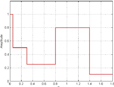
For input of system nonlinear squre wave is used, this wave is shown in Figure 3.15.

22

As seen in Figure 3.15, the maximum amplitude of this wave is 1 and miminum value is 0.1. The time interval is between 0 and 1.8. In Simulink the used block is as below.

3.6 A Brief Conclusion

Figure 3.17 shows the closed-loop DC motor control system with PID controller. In this model the PID controller controls the output of DC motor with some coeficient of adaptive mechanism. For adaptive section there is just one coeficient [26].

Figure 3.15 Input of the Proposed Adaptive Control Model

23

In proposed method integral of the reference model and subtract of the reference and DC motor output are used. The adaptive mechanism of porposed model is shown in Figure 3.17.

As future work, the adaptation mechanism can be designed using different theories for the exact model of the DC motor, also can be implemented. For this system input lookup table and time variant are used. For real time work it can be integrated on SCADA systems.

4. GENERAL STRUCTURE OF DESIGNED AUTOMATION SYSTEM

The system is composed of three station, three PLCs providing data exchange and equipment control and a computer that the SCADA software is running (Figure 4.1).

Figure 4.1 Components and General Structure of the Designed System Figure 3.17 Closed-loop DC Motor Control System

24 4.1. SCADA Interface

The systems that collect the field data as continuously and real-time from devices used in proces and automations such as programmable controller, provide to the operators (users) monitoring of various factors affecting the production according to defined criterias from a central point by evaluating this information and used in order to ensure the possibility of remote controlling may be called supervisory control and data acquisition (SCADA) [8]. SCADA system is a combination of data collection and telemetry; performs data collection and sends data to the center, makes analysis and then displays this data on the operator screen. SCADA system displays and controls the field equipments as well with represented objects.

By using dynamic object drawing tools, monitoring the desired process can be simulated in a way that represents the reality and warnings can be made remarkable. SCADA softwares include features such as graphics, motions, sizing, flashing that can provide ease of use to operators.

The screen of the stations are accessible from the button in the main screen which stations' name on. Stations can be started and parameters of the system can be adjusted manually from the screen when desired. The circle next to the running station becomes green and the text 'istasyon hazır' appears.

25 4.2. Siemens SIMATIC S7-200 PLC

Programmable logic controller is an industrial computer which collects information about the connected system, sends this informaion to the control center via a specific communication environment, implements the commands from the control center. PLCs provide appropriate control environment to software programs for on the one hand fulfill the process functions while also transmit the information and data to SCADA system [10].

SIMATIC S7-200 family of programmable controllers are improved devices for the realization of control circuits of small automation systems with 64 input, 64 output and feedback control circuits that require 12 analog input, 4 analog output point [9].

In this study, S7-200 CPU224 model PLCs are used. Prototype programs suitable with the system hardware are installed to PLCs by using SIMATIC/Step-7 program and firstly communication operations of the PLCs are provided. As PPI address, numbers 2, 3, 4 to PLCs and number 1 to SCADA control system are assigned.

Figure 4.2 Main SCADA Screen Figure 4.3 S7-200 Working Principle [9]

26

5. COMMUNICATIN IN THE AUTOMATION SYSTEM

5.1. S7-200 Network Communication

The S7-200 supports a master-slave network and can fuction as either a master or a slave in a Profibus network, while STEP 7-Micro/WIN is always a master.

A device that is a master on a network can initiate a request to another device on the network. A master can also respond to requests from other masters on the network. Typical master devices includes STEP 7-Micro/WIN, human-machine interface (HMI) devices such as TD 200. On the other hand, a device that is configured as a slave can only respond to requests from a master device; a slave never initiates a request. For most networks, the S7-200 functions as a slave. As a slave device, S7-200 responds to requests from network master device, such as an operator panel or STEP 7-Micro/WIN [9].

5.2 Setting the Baud Rate and Network Address

The speed that data is transmitted across the network is the baud rate, which is typically measured in units of kilobaud or megabaud. The baud rate measures how much data can be transmitted within a given amount of time. For example, a baud rate of 19,2 kbaud describes a transmission rate of 19200 bits per second [9].

Every device that communicates over a given network must be configured to transmit data at the same baud rate. Therefore, the fastest baud rate for the network is determined by the slowest device connected to the network [9]. In this study common baud rate was adjusted as 19,2 kbps.

The network address is a unique number that it is assigned to each device on the network. The unique network address ensures that the data is transferred to or

27

retrieved from the correct device. The S7-200 supports network addresses from 0 to 126.

Typically, the network address 0 for STEP 7-Micro/WIN is not changed. If the network includes another programming package, it might need to change the network address for STEP 7-Micro/WIN. In the following figure adjusting the communication settings of the STEP 7-Micro/WIN is shown (Figure 5.1).

The baud rate and network address must also configure for the S7-200. It is also done by using STEP 7-Micro/WIN. The addresses of the three S7-200 in the system; for unloading and carrying station is 2, for processing station is 3, for test and seperation station is 4. Adjusting the address and baud settings of the S7-200 is shown in the Figure 3.2. After adjusting the settings throug STEP 7-Micro/WIN, it must be download to S7-200.

28 5.3. Profibus

The protocols are made for transfering information via any enviroment between two or more devices which use different languages. For performing quick, safe and understandable data communication in any protocol all details about information transfer and control are specified and fixed.

Profibus is an international fieldbus communications standard for linking process control and plant automation modules, it is an open field line protokol and independent from the producer. These are based on the international standards (EN 50170, EN 50254 ve IEC 61158). Profibus is a data way which has nearly 650 members and is supported by many research institutes. It provides communication

Figure 5.2 STEP 7-Micro/WIN Communication Ports

29

between devices of different producers while doing this does not need any special interface. This data way system is widely applied in areas such as complex communication processes or critical applications with high speed [12]. Profibus networks typically have one master and several slave I/O devices. The master device is configured to know what type of I/O slaves are connected and at what addresses [9].

The profibus cables which connect three PLCs and provide communication have connectors. These connectors have two sets of terminal screws to allow you to attach the incoming and outgoing network cables. The connectors also have switches to bias and terminate the network selectively. Figure 3.4 shows typical termination for the cable connectors. Cable must be terminated at both ends.

5.4. Configuring the OPC Server with S7-200 PC Access

OPC is the abbreviation of OLE (Object Linking Embedded) for Process Control and it is a standard unit in automation technologies. This term is a method that provides managing, reporting and observing the different brand of PLC and industrial devices on a single source [13].

Figure 5.4 Profibus Cable Connections [9]

30

Figure 5.7 PC Access Communication Settings

Setting up a OPC server with PC Access program for Siemens S7-200 PLCs is as follow.

A new project is created and the controller is marked (for example MicroWin(USB)). As access point of the application it must be set 'MicroWin' with existing communicaitons connection to the S7-200. In this study the project is 'MicroWin(USB) and the PLCs are PLC_Y0044A, B, C. The network addresses of the PLCs PLC' lerin network adresleri 2, 3, 4'tür. Communication addresses and baud rates must be same with STEP 7-Micro/WIN and S7-200.

31

The items must be add to PC Access program according to match the tags which will build the SCADA screen (Figure 5.8).

5.5. WinCC Flexible

In SCADA system variables where data communication with PLC is done and the tags which are expressing these variables must be defined. Elements using on the SCADA screen such as buton, switch, motor are activated with defined tags. For every tag it is determined to be read and written information from which data block or address. In study, to perform the SCADA interface, SIMATIC WinCC Flexible 2008 is used.

Figure 5.8 Adding Items to the PLCs

32

6. UNLOADING AND CARRYING STATION

The basic software of this system is providing movement of the materials one by one from material reservoir to carrying unit with unloading piston. Then the materials are carried to the next station by the carrying unit.

The stuffed materials in reservoir are driven forward with unloading piston till getting signal from the limit switch. The limit switch generates signal when material touched to the switch and the carrying piston goes down to get the material. Unloading piston waits until the material is vacuumed. When the vacuum switch generated signal, the unloading piston releases the material and moves back. The carrying piston moves right after uplifts the material. When the unit came right, right limit switch generates signal and the motor of the carrying unit is stopped, then carrying piston begins to go down. When the material reached down, it is released by stopping vacuum and the system returns to its initial position for another material. When material ends, because of the limit switch cannot generate a signal from forward position of the unloading piston, the piston moves back and the system stops.

33 6.1. Components Used in the System

6.1.1. Limit Switch

The automatic operation of a machine requires to use the switches actuates with its movement. Limit switch is a type of circuit element allowing or stopping a new operation in movable systems, it transforms the mechanical movement into electircal signals in order to actuate electrical circuits. The internal structure of the limit switch includes a normally opened down contact and a normally closed up contact. When the movable part physically touches the head of the limit switch the contacts changes position. The contacts return to their neutral state when the pressure is removed by an internal spring [15].

In this station, the limit switch is used to determine the forward position of the unloading rod and whether the carrying unit is on right or left position.

6.1.2. Manometer and Dryer Module

It is important for pneumatic systems to have the supply of air clean, dry and with a stable pressure. Conditioners are used at the entrance of the pneumatic systems where the air is transferred through pipes from the cylinder in order to supply the optimum pressure and volume of the air to be used in the system [16, 17]. Manometers and dryers are used together in the conditioner of this system.

Increasing and decreasing of the air requirement cause to drop of working pressure which leads unwanted situations like power loss. Pressure regulators are used to supply pressure at a stable level and limit the working pressure for the accurate operation of the system.

As the fundamental parts of the process control, the measuring devices can be classified in two categories as electronic and mechanical. Although it is possible to control the process with electronic measuring devices in PLC and SCADA systems, reading these values in the field accurately is important in terms of operational safety. In this context, manometers are inevitably important for measurement [16,

34

17]. They are measuring devices which measures the air pressure in the system. A pressure of 5-6 bars is required for the accuracy of this system.

Water vapour in the air supplied to the system shortens the life of circuit components as they wear out quickly. Therefore, dryers are used before transportation of air to the system [16]. Water accumulates due to water vapour in the air stored within the system. The accumulated water at the bottom of the conditioner needs to be released by opening water evacuation valves.

6.1.3. Solenoid Valve Group

Valves are pneumatic components that evacuate or release pressured air or control the flow of its direction, its amount and its volume. Solenoid valves help to control the direction of the flow of the compressed air required for the operation of the system. Thereby, it ensures the accurate movement of the pneumatic components in the desired direction. Solenoid valves work on electrical energy and ensures the automatic control of the air. Application of electrical signals to the desired valve causes the compressed air to be transported from the related cylinders [18, 16].

35 6.1.4. Unloading Unit

This unit, provides unload of these materials from the reservoir by pushing the materials in the reservoir to the position which carrying piston will take. The forward position of the unloading rod is determined when the limit switch is pressed. Pneumatic pistons are used to perform this process.

Pneumatic pistons are used in all industrial areas to fulfil functions such as transportation, packaging and forwarding and Industrial fields using these pistons increase day by day. The working principle of the piston is to let compressed air to the air chamber providing the release piston and the piston rod a linear movement. Pneumatic pistons transform the energy of the compressed air into a movement of linear push or pull [18]. The pneumatic pistons ensure the forward/backward movement of the unloading rod in this system.

36 6.1.5. Vacuum Generator

The evacuation of the air particles from a defined space leads to pressure difference between the atmosphere and the related space. Vacuum is produced as the air pressure of the surrounding is lower than the atmospheric pressure. The vacuum level depends on the amount of air evacuated from the surrounding of a defined space. Higher evacuation leads to a more powerful vacuum [16]. The device used to produce vacuum in this system is a vacuum generator.

The compressed air allowed to flow through the nozzle of a vacuum generator produces vacuum. Compressed air is allowed to flow from the A component of the vacuum generator shown in the picture. As the air expands from the nozzle of D towards B the speed of the air increases to a high level and starts to produce vacuum from C [16]. Noise reducing mufflers should be used as compressed air flow will generate a high level of noise. The schematic principle of the operation of the system via a vacuum generator is shown in Figure 6.4.

Figure 6.4 Cross-section of Vacuum Generator

[16]

37 6.1.6. Vacuum Switch

It is an electronic device measuring the reverse compressed air at the part where air is allowed in to the vacuum switch. This device provides feedback whether the materials are handled as a result of the vacuum. When the piston fails to handle the material the vacuum switch will not produce any signals as the air suction will be high. When the piston is needed to move after vacuumed the material, PLC programme flow will be run according to the signal produced by the vacuum switch.

6.1.7. Carrying Unit

The carrying unit is a mechanism which moves both in the right and left axial direction to deliver and take the material held by the carrying piston. The step motor allows the left or right movement.

As can be understood from the name, the step motors move step by step, namely they proceed one step at a time when one of the bands gets energy. The step motor is an electro-mechanic device which transforms the electric power into rotating movement. When there is electric power, the impeller and the shaft linked to it start to rotate step by step. To operate the step motors in the required way with the right speed, consecutive pulses should be applied. This process is conducted with the driver circuits [20]. The step motor of the unit is propelled through the step motor driver circuit located in the panel. This driver takes pulses from the PLC.

38

The driver circuit of the step motor have two inputs which are moved to the panel. These are Axial R/L and Axial CP. The axial R/L input is the one which determines the rotating way of the motor. When the axial R/L is "0", a movement in the left way is achieved. And when it is "1", it turns right. For the step motor to complete its rotation, a sequence of pulse should be applied to the axial CP input. The frequency of the applied pulse is the factor which determines the rotation speed of the step motor.

7. PROCESSING STATION

The basic software of this station is to transport the material transferred to rotary table to the following station via a carrying unit after going through a carrying unit.

As the material transferred from the previous unit is placed at the entrance of the rotary table, optical sensor produces a signal and the rod starts its movement after a short period. The table stops when the material arrives at the process unit. The materials are compressed by the piston. The drill starts to work and move downwards. When the drill arrives at the bottom limit, it continues to carry out the process for a while and then moves upwards. When it reaches the top limit it stops and the piston releases the material. At the end of the process, the table rotates and stops at the point where the material will be received by the carrying unit. At this

39

point, the signal from the inductive sensor propels the piston to move downwards to vacuum the material. Then, it starts to rotate towards its right. When signal is received from the right limit switch at the carrying unit piston moves down, shuts off the vacuum and transports the material to the following station. After the material is transported system is restored and on stand by for the new material.

7.1. Components Used in the System

7.1.1. Optical Sensor

With a source of light falling on an optical sensor is produces visible or infrared light. This light is directed towards the object needed to be perceived [21]. If the optical sensor is reflected from the object as in this system, perception occurs when the level of reflected light reaches the defined threshold value.

40

The start of the system is propelled through the perception of the object left at the rotary actuator via the optical sensor. Light emitted from the sensor hits the object, thus it will be reflected at a certain rate and the presence of an object in front of the sensor will be perceived. The diagram related to the electrical wiring of the optical sensor is shown in the Figure 5.3. BN (+), BU (-) supply pins work at 10-30 DC voltage and requires current of approximately 100 mA. BK is normally open, WH is normally closed probes and the BK probe of the sensor is used in the system. The setting for the sensitivity of the system can be adjusted according to the reflective characteristics of the objects.

7.1.2. Inductive Sensor

Inductive sensor detects metallic or conductive objects without touching them whether they move or not. Inductive sensor is composed of coil, oscillator, trigger and output. The current applied to the sensor causes the oscillator to rise and fall and the sensor creates an electromagnetic field in the close surrounding of its sensing surface [21]. The presence of a metallic object in the operating area affects this magnetic field. This change is processed in the electric circuit of the sensor and the sensor changes the output signal. Therefore, the presence of a metallic object

Figure 7.3 Electirical Wiring Diagram of the Optical Sensor [13] Figure 7.2 Optical Sensor Working Principle [22]

41

entering the sensing area of the sensor is detected. The changing output signal is evaluated by PLC.

LED indicator of the inductive sensor which is placed on the processing station will give out light when metallic objects are detected. The position of the rotary actuator is controlled in that station. with the inductive sensor. These sensors produce the required signals to stop the engine of the rotary table by detecting the metallic objects fastened under the arms of the table.

7.1.3. Rotary Table

A rotary table is a device used to process materials and works sensitively in terms of positioning. It provides the working of the processing unit in specific times around a fixed axis. The actuator directs the incoming material to the operation point by turning right, secondly, it rotates the material towards the following station to receive the material. The position where the table is expected to stop is detected by inductive sensors fastened on arms of the table.

Figure 7.4 Inductive Sensor Working Principle

42

The rotation of the table is ensured via DC motor with a reductor. Reductor is a closed gearing mechanism designed for adjusting the high speed rotation of the electrical motors to the level required for the related machines [23].

7.1.4. Processing Unit

The processing unit consists of a drilling mechanism which conducts drilling, grinding and sweeping operations according to the tools attached to the pin of the processing unit.

Figure 7.6 Rotary Table [13]

43

The drilling machine is mounted to a threaded mechanism which allows it to move up and down. The DC motor makes the movement and rotation of the machine possible. The on/off switch should be turned on for the drilling machine to start when the signal comes from PLC.

7.1.5. Carrying Unit

This unit has the same working principle as the carrying unit at the unloading and carrying station. The difference of this station is that the rotation towards left or right is provided by a DC motor. The DC motor of the unit is propelled through the direction driver circuit of the DC motor located in the panel. The driver circuit of the DC motor have two inputs which are moved to the panel. These are Axial Left and Axial Right. When the Axial Left is "1", a movement in the left way is achieved. And when the Axial Right is "1", it turns right.

8. TEST AND SEPERATION STATION

The basic software of this station distinguishes the materials by their type (metal, white, black). When the material delivered on the starting point of the band is detected by the optical sensor, the band starts to move after a little while. This duration can be control from the monitoring screen. When the object is passing by the inductive sensor, the sensor produces a signal and metal distinguisher closes so that the material falls down to the metal section. If the material is not metal, the signal received from optical contrast sensor is evaluated to determine the colour of the material. If the material produces a signal at the optical contrast sensor, it is concluded to be white, if it does not produce a signal it is concluded to be black. Gain scheduling algorithm is used in this station to control the band speed. If other sersor fastened to this unit for recognization of the material type, the band speed can adjust itself according the sensitivity of this materials.

44 8.1. Components Used in the System

8.1.1. Siemens TD-200 Operator Panel

TD 200 is a text display unit which can only be mounted to the S7-200 device and has a space for 2 lines and 20 characters for each line. This device can be programmed to display the the text messages coming to S7-200 and the variants of the application [2]. In the system, TD 200 is connected to the Port 0 of the last station (testing and separating).

Figure 8.2 TD 200 [9]