© 2013 Pakistan Journal of Statistics 59 VISUALIZING DIAGNOSTIC OF MULTICOLLINEARITY:
TABLEPLOT AND BIPLOT METHODS B. Baris Alkan1§and Cemal Atakan2
1 Faculty of Sciences and Arts, Department of Statistics, Sinop University, 57000, Sinop, Turkey. Email: [email protected]
2 Faculty of Science, Department of Statistics, Ankara University, 06100, Ankara, Turkey. Email: [email protected] § Corresponding author
ABSTRACT
In this study we tried to bring out the importance of two methods used for visualizing multicollinearity diagnostics. The first method is called Tableplot (see Friendly and Kwan, 2009). Through this technique, multicollinearity diagnostics ideas are combined with a visualizing approach. The second method is called Biplot (see Gabriel, 1971; Gower and Hand, 1996). The biplot technique is used for demonstrating significant properties of multivariate data structure. Both of these approaches have been examined by one real and three artificial data. Results indicate that Biplot method is preferred to instead of Tableplot for too large condition indexes.
KEYWORDS
Multicollinearty; Biplot; Tableplot; Visualizing approach. 1. INTRODUCTION
Multicollinearity is considered as an important issue within the context of multiple regression analysis which refers to high correlation among the explanatory variables. This high correlation indicates the multicollinearity, but the opposite is not always true. In other words, if there is multicollinearity between the explanatory variables, the correlation between pairs of these variables may not be high. Multicollinearity causes certain adverse effects on multiple regression analysis, such as less reliable estimates and large standard errors for regression coefficients.
Estimation problems arising as a result of high correlation (or close dependence) among the explanatory variables in multiple regression models were first discussed by Belsley et al. (1980). They examined the diagnostic methods for the determination of sources causing multicollinearity. Moreover, they gave variance decomposition proportions, condition indexes and eigenvalues from the multicollinearity diagnostics methods in a single table. Then Belsley (1991a) have conducted several studies toward the visualization of diagnostic methods for multicollinearity.
Chatterjee and Price (1977), Weisberg (1980), and Hocking (1983) argued various methods in order to identify multicollinearity, most of which were based on the correlation matrix or its inverse.
Friendly and Kwan (2009) considered multicollinearity as a complex issue like a puzzle identification. They have suggested a visual structure called TablePlot. They also described a biplot method called “collinearity biplot” for the diagnostic of multicollinearity.
The main objective of this study is to show the importance of the methods of tableplot and collinearity biplot for visualizing diagnostic of the multicollinearity. The two methods were matched by one real data and three artificial data and their performances and features were examined in details.
The remaining sections of this study have been organized as follows: Section 2 presents the data and methodology. The empirical results are explored in Section 3, and the final section involves the concluding remarks and our evaluations
2. DATA AND METHODOLOGY
Real Data
This paper uses the data of twenty nine Europe & Central Asia (all income levels) countries to demonstrate the importance of two visualizing multicollinearity diagnostics methods. The variables are defined as follows: The Gross Domestic Product (GDP) per capita annual percentage change (GDP as Logarithm); Fertility Rate (FR as Logarithm), total (births per woman); consumer prices inflation rate annual percentage change (INF); Urban Population (UP); Mortality Rate (MR as Logarithm), infant (per 1000 live births); total unemployment rate as a percentage of total labor force (U); household final consumption expenditure per capita growth annual percentage change (C).
The data used in the study was gathered from the Databank of the World Bank (for the year 2008). The countries were chosen by the availability of the data within the Europe& Central Asia countries. Data set was given in Table 1.
The data set was firstly analyzed with R ver.2.11.1 (R Development Core Team 2010) program. It was observed that the assumptions were satisfied with the logarithmic transformations of the variables of GDP, FR and MR.
Artificial Data
Artificial data sets were used in order to explore two visualizing diagnostic methods of multicollinearity. Two different visualizing methods were applied on these artificial data sets.
In this study, one hundred observations (n) were chosen, since it was quite adequate to display coherent results for artificial data set.
Artificial data were constructed with algorithm as follows:
Step 1 Mrandn p
, to generate random pxp matrix from a standard normal distributionStep 2 SM MT , multiply it by its own transposition A positive semi-definite matrix is obtained with the first two steps.
Step 3 X mvnrnd zeros p
,1 , ,S n
, generated an nxp matrix X of random vectors chosen from the multivariate normal distribution with mean zero vector, and covariance matrix S. This matrix is called the matrix of explanatory variables in our study.Step 4 y X
:,1 X
:,2 ... X
:,p normrnd
0,1,100,1
, to obtain response variable, where p is number of explanatory variables and takes 10,15,20 respectively; n is taken as 100. This vector is called as the vector of response variable in our study. The number of the response variable was taken as one. In addition, the weak and strong multicollinearity conditions on the two applications are discussed. For the case of weak multicollinearity, the data were generated as follows:
X i =normrnd 0,1,100,1 , i1,...,p.
Y=X 1 +X 2 +...+X p +normrnd 0,1,100,1
where p5,n100.
For the case of strong multicollinearity, we used Hald’s Cement Data (Wood et al., 1932) with 13 observations on the 5 variables.
We have used MATLAB script and functions for the solution of algorithm.
Methodology
In this study, we have used the visualizing diagnostic methods known as collinearity biplot and tableplot in order to examine the relation between variables for the real and the artificial data. The tableplot combines multicollinearity diagnostic ideas with visualizing approach, developed by Kwan (2008). The biplot technique is used for showing significant properties of multivariate data structure initially introduced by Gabriel (1971) and later developed by Gabriel (1978), Gabriel and Odoroff (1988), Gower and Hand (1996), Gower (2004). The biplot could be considered to be a multivariate version of dot scatter plots which have been used for analyzing bivariate data. This technique is based on the singular value decomposition analysis.
The following subsection summarizes the theoretical background of the biplot and the tableplot methods.
Table 1:
Data set of twenty nine Europe & Central Asia (all income levels) countries
LOGGDPa LOGFRb INFc UPd LOGMRe Uf Cg
0,5027 1,8271 3,1823 67,1600 0,5441 3,8000 0,0380 0,6522 1,9884 4,4892 97,3600 0,5911 7,0000 0,7152 0,7830 1,7580 6,0670 57,2800 0,6721 8,4000 1,0380 0,8031 1,8663 6,3551 73,5000 0,4771 4,4000 2,6965 0,5314 1,9379 3,3995 86,6800 0,5441 3,3000 -1,1530 1,0156 1,8417 10,3656 69,4600 0,6721 5,5000 -4,8953 0,6092 1,8014 4,0660 63,3000 0,4150 6,4000 1,2462 0,4493 1,8885 2,8139 77,3600 0,5315 7,4000 -0,0289 0,6183 1,7853 4,1524 61,0000 0,4771 7,7000 2,7707 0,6078 1,7877 4,0535 61,3400 0,5682 3,0000 -9,1408 0,5248 1,8330 3,3478 68,0800 0,5315 6,0000 -3,1607 1,1876 1,8333 15,4032 68,1200 0,8633 6,7000 -1,5223 0,5315 1,9161 3,4003 82,4400 0,2553 5,8000 -5,0780 0,8585 1,8254 7,2185 66,9000 1,0212 5,1000 2,8448 1,1063 1,6208 12,7744 41,7600 1,1818 33,8000 6,4999 0,3953 1,9129 2,4848 81,8200 0,5911 4,0000 0,7519 0,5759 1,8892 3,7662 77,4800 0,4624 2,8000 0,4434 0,6384 1,7876 4,3494 61,3200 0,7634 2,6000 5,9041 0,4134 1,7742 2,5904 59,4600 0,5052 7,1000 1,6420 0,8948 1,7343 7,8483 54,2400 1,0492 7,6000 8,5675 1,1495 1,8624 14,1078 72,8400 1,0756 5,8000 10,8113 1,1096 1,7163 12,8707 52,0400 0,8195 13,6000 8,0322 0,6626 1,7525 4,5982 56,5600 0,7782 9,5000 5,8844 0,6095 1,8872 4,0688 77,1200 0,5563 11,3000 -2,0779 0,5362 1,9271 3,4370 84,5400 0,3802 6,2000 -0,7847 0,3843 1,8662 2,4225 73,4800 0,6128 3,4000 0,0490 1,0189 1,8368 10,4441 68,6800 1,2989 9,4000 -1,5445 1,4020 1,8324 25,2319 67,9800 1,1367 6,4000 11,1165 0,6014 1,9540 3,9937 89,9400 0,6721 5,6000 -0,2238
a-) GDP as Logarithm, GDP per capita growth (annual %); b-) FR as Logarithm, Fertility rate, total (births per woman); c-) INF, Inflation, consumer prices (annual %);
d-) UP, Urban population (% of total);
e-) MR as Logarithm, Mortality rate, infant (per 1,000 live births); f-) U, Unemployment, total (% of total labor force);
2.1 Overview to Multiple Linear Regression Model
In general, the multiple linear regression model is as follows:
y X (2.1)
where y is an n vector of response variable. 1 X is the n p full-rank. β is the p1 vector of regression coefficients, and ε is an n1 vector of random errors,
ε 0,
ε 2IE Var . The least squares estimator of β is given by
X XT
1X yT .The variances of the estimators of the parameters are as follow:
2
T
1Var X X (2.2)
2.2 The Negative Effects of Multicollinearity
The presence of multicollinearity among the explanatory variables causes several problems such as inflated variances and covariances, inflated prediction variance, problems in interpreting the significance values and confidence regions for estimated parameters, unreliable t and F statistics (Farrar and Glauber, 1967; Silvey, 1969; Marquardt, 1970, Marquardt and Snee, 1975; Andrew and Watts, 1978).
2.3 Diagnostics for Multicollinearity
Variance inflation factors (VIFs), condition indexes, condition number and variance decomposition proportions were computed to scale the impact of collinearity. These concepts were explained in the following subsections.
2.3.1 The Variance Inflation Factor (VIF)
Measure of collinearity is the variance inflation factor for the j-th regression coefficient VIFj. The variance inflation factors were computed from the sample correlation matrix of the explanatory variables.
2 / 1 1 j j VIF R (2.3)
If VIFj is equal to 1 then 2
j
R is zero, that is Xj is not linearly related to the other explanatory variables. If VIFj then R2j is one, when Xj tends to have a perfect
linear association with other explanatory variables, where 2
j
R is the coefficient of multiple determination of Xj on the other explanatory variables (Rawlings et al., 1998; Friendly and Kwan, 2009).
Sampling variances of the nonintercept parameter estimates can be expressed with equation (2.4). The variance of the j-th regression coefficient can be shown to be directly proportional toVIFj,
1 2 2 β X X x x T j T j j j Var VIF (2.4)where xj is the j-th observed value of the column of the centered X matrix (Theil, 1971; Berk, 1977; Belsley et al., 1980; Rawlings et al., 1998; Friendly and Kwan, 2009).
The diagonal elements of
X XT
1 matrix in equation (2.4) are given with
2
1 1Rj (Rawlings et al., 1998).
VIF values greater than 10 for each variable and average VIF greater than 6 are the indications of the multicollinearity (Hocking, 1983).
2.3.2 Use of eigenvalues
Eigenvalues are important for the methods such as condition number, condition index, variance decomposition proportions in terms of multicollinearity diagnostics. Multicollinearity diagnostics methods use the eigenvalues of X XT or
XX
R matrix. RXX is the correlation matrix among the explanatory variables (Rawlings et al., 1998).
Condition Index (CI)
CI can be computed for the each eigenvalue. The eigenvalues are sorted in descending order, where the largest eigenvalue with . The condition indexes are 1 obtained with CIj max j, where j1, 2,...,p; p is the smallest eigenvalue. Some
authors use CI as the square root of max j (Paulson, 2007). For instance, SAS and R program are used indication of CIj .
According to Belsley (1991b), more than 30 CI shows harmful, and more than 100 CI is an indicator of potential problem in estimation.
Condition Number (CN)
The CN is obtained with the ratio of max min . If CN is over than 100, there
exists a strong multicollinearity (Belsley et al., 1980; Rawlings et al., 1998).
Variance Decomposition Proportions (VDP)
Spectral decomposition of the correlation matrix of the explanatory variables is given with RXX V VT, where Λ consists of diagonal elements of eigenvalues of RXX in
descending order. Additionally VIFj can be obtained with diagonal elements of RXX1 . In that case, VIFj is written as 2
1 p j jk k k VIF v
. vjk is the jth element inV . Thus VDP is obtained (Belsley et al., 1980; Fox, 1984; Rawlings et al., 1998; Friendly and Kwan, 2009) as follow2 2 2 1 jk jk k jk p j k jk k k v v VDP VIF v
(2.5)According to Belsley (1991a and 1991b), if the VDP is greater than 0.5 then multicollinearity between two or more explanatory variables may occur.
2.4 Tableplot
Understanding of overall structure from findings on a single table in statistical analysis is not always possible. In such cases, the uses of the graphical methods are extremely important. Many graphical methods were proposed depending on the type of data structure for the accurate interpretation of the results of the analysis in the literature.
In this study, we innitially have used a method called Tableplot for visualizing diagnostics of multicollinearity proposed by Friendly and Kwan (2009). Tableplot is a combination of tables and graphics. The tableplot provides graphical presentation of existing multicollinearity diagnostic methods. It also provides more important foreground information of contributory to multicollinearity hidden within the complex numerical data.
The first column of the Tableplot consists of condition indexes in a descending order. The condition indexes are shown by white squares in column 1. This first column is scaled according to the size of condition indexes. Considering these scales, backgrounds of the rows of the first column are colored. In addition, other columns of the Tableplot are given with intra-colored circle according to VDP (multiplied by 100). The color of this circle indicates the contribution to multicollinearity.
Column 1 indicates the values of the condition indexes, CIj . According to Friendly and Kwan (2009), in the Tableplot, green (‘‘OK’’) shows CIj <5 i.e. no multicollinearity; yellow (‘‘warning’’) shows 5 CIj 10 i.e. near-perfect multicollinearity and red (‘‘danger’’) shows CIj 10 i.e. perfect multicollinearity. The coloring of the other columns is done according to VDP (multiplied by 100). Here, {0-20, 20-50, 50-100} rates corresponding to the colors {White, Pink, Red} respectively.
2.5 Classic and Collinearity Biplot
Biplot method is used for the graphical analysis of the multivariate data structure. It is used for exploring the hidden in details, significant properties of multivariate data. The biplot can be considered as multivariate equivalents of dot scatter plots which have been used for analyzing bivariate data (Gabriel, 1971; Gower and Hand, 1996).
Any X n p: matrix with r rank can be factorized as X GHT where the matrices :
G n r and H p r: represent the samples and variables respectively. There are different specifications for G and H, depending on what is to be optimally represented
in the biplot. It appears that the cosine of the angle between any pair of vectors is the most important aspects for the use as diagnostics for multicollinearity. It is therefore advisable to choose G such that G G IT (Gabriel, 1971).
The graphical Biplot approach in multiple regression analysis is used for the correlation matrix
RXX
of centered explanatory variables
X . This biplot is a graph together with principal component coefficients for the variables and principal component scores for the observations in lower dimensional space (two or three) with principal component analysis of RXX. In this graphic, observations are represented with points andvariables are represented with vectors. It is called a classical biplot and created with the first two or three dimensions, corresponding to the biggest eigenvalues of RXX (Jolliffe, 2002; Friendly and Kwan, 2009). The orthogonal projections of observation points onto variable vectors in biplot give approximately the elements of centered data matrix. Cosine of the angles between any pairs of vectors approximates the correlation between the variable vectors. In the graphical representation, correlations between each variable vector and the coordinate axes are also obtained approximately with the cosine of the angles between them (Gabriel, 1971; Gower and Hand, 1996; Aitchison and Greenacre, 2002).
The use of biplot method in the visualization diagnostic of multicollinearity problems is proposed by Friendly and Kwan (2009). This version of biplot is called collinearity biplot. According to Friendly and Kwan (2009), classic biplot gives useful information about data set. But if the comments of the classic biplot are used for multicollinearity diagnostics, these comments can be misleading. So they have used collinearity biplot created with the smallest dimensions. Small dimensions have large condition indexes and these indexes are the indication of multicollinearity.
3. SUMMARY OF THE RESULTS
The results of Analysis for Real Data
In results of analysis measure of the goodness of fit of model is very good with
2 0.927
R . Table 2 presents the parameter estimates and their standard errors. According to t statistics in Table 2, INF is a significant. VIFs for FR and UP explanatory variables are greater than 10. So these variables may be cause collinearity problems.
Table 3 present the condition indexes and variance decomposition proportions for the model. The modified version of Table 3 is also given Table 4. Table 4 indicates the contributions of the variables to multicollinearity in the smallest two dimensions (dimension 5 and dimension 6). We receive the last two rows in condition that indexes are greater than 10. Table 4 indicates near linear dependency between LOGFR and UP explanatory variables in dimension 6 and between LOGMR and INF in dimension 5.
Table 2:
Parameter estimates and VIFs for data set Variable DF** Parameter
Estimate Standard Error t-Value p-Value Variance Inflation
LOGFR 1 -1.89016 2.96402 -0.64 0.5302 223.70943 INF 1 0.04473 0.00471 9.50 0.0001* 2.44856 UP 1 0.00992 0.01770 0.56 0.5809 193.28279 LOGMR 1 0.16242 0.09557 1.70 0.1033 2.58381 U 1 -0.00143 0.00612 -0.23 0.8181 4.97038 C 1 -0.00453 0.00443 -1.02 0.3181 1.75220 * p<0.05, **DF, degrees of freedom Table 3:
Condition indexes and variance decomposition proportions Dimensions ConditionIndex
Variance Decomposition Proportions
LOGFR INF UP LOGMR U C
Dimension 1 1.000 0.000 0.007 0.000 0.002 0.010 0.007 Dimension 2 2.228 0.001 0.005 0.001 0.000 0.000 0.483 Dimension 3 3.937 0.001 0.010 0.004 0.001 0.719 0.062 Dimension 4 4.785 0.003 0.566 0.005 0.002 0.021 0.375 Dimension 5 10.307 0.003 0.400 0.024 0.849 0.121 0.070 Dimension 6 32.118 0.992 0.012 0.965 0.146 0.130 0.003 Table 4:
Modified condition indexes and variance decomposition proportions Dimensions ConditionIndex
Variance Decomposition Proportions (x100)
LOGFR INF UP LOGMR U C
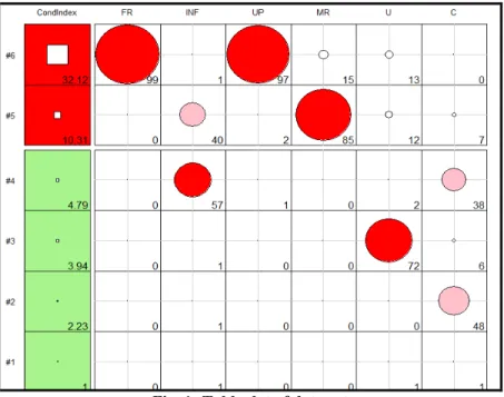
Dimension 6 32.12 99 1 97 15 13 0
Dimension 5 10.31 0 40 2 85 12 7
Note: Variance decomposition proportions (VDP) greater than 0.40 is shown as bold. Figure 1 shows a tableplot of all condition indexes and variance decomposition proportions. According to Figure 1, the top two rows are painted as red for the condition index, the contributions of the variables for the smallest dimensions are seen in Table 4. Other dimensions between 1 to 4 are painted as green. That means there is no collinearity problem in the dimensions between 1 to 4.
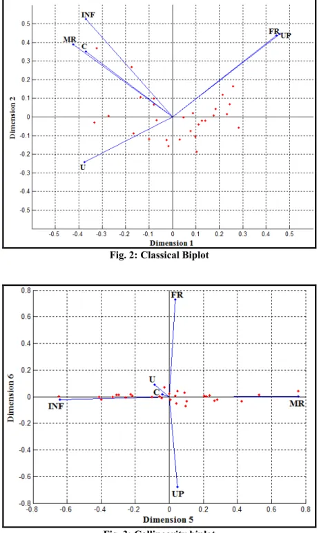
The classical biplot in Figure 2 presents relations of between observations and explanatory variables. It also gives the variation of explanatory variables on the lower dimensional space (two largest dimensions). These two dimensions account for 78% of the total variation in the 6-dimensional space. All the total variance can be explained by six dimensions. 57.43% of the total variance is explained by the first dimension and the 20.48% of the total variance is explained by the second dimension. 9.89% of the total variance by the third dimension and the 7.83% of the total variance is explained by the fourth dimension, 4.33% of the total variance is explained by the fifth dimension and 0.04% of the total inertia is explained by the sixth dimension. If Figure 2 is examined, two clusters of highly related variables are seen. While the first cluster is described with FR&UP variables, the second cluster is described with MR&C&INF variables. There’s also negative high correlation as relativity between FR&UP and U variables. These comments are not useful in terms of diagnosis of multicollinearity since the collinearity problem is hidden in least dimensions.
Fig. 2: Classical Biplot
The collinearity biplot for the smallest two dimensions in Figure 3 accounts for 4.37% of the total variation. This biplot approach supports the comments of Table 4 and Tableplot. According to Figure 3, the variables of FR&UP on Dimension 6 and the variables of INF&MR on Dimension 5 are effective. The effects of U&C variables on Dimension 5 are quite small. The results of collinearity biplot and tableplot for real data sets are parallel.
The results of Analysis for Artificial Data
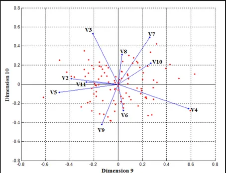
Figure 4 shows a tableplot of all condition indexes and variance decomposition proportions for artificial data, p=10, n=100. According to Figure 4, the top two rows are painted as yellow for the condition index, the contributions of the variables for the smallest dimensions are seen in this tableplot. Other dimensions between 1 and 8 are painted as green. This means that there is no collinearity problem in the dimensions between 1 and 8. The collinearity biplot for the smallest two dimensions in Figure 5 account for 0.61% of the total variation. According to Figure 5, the variables in the range of V6-V10 on Dimension 10 and the variables of V2,V4 and V5 on Dimension 9 are effective. This biplot approach supports the comments of Figure 4.
Fig. 4: Tableplot of artificial data for p=10, n=100
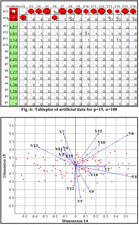
Figure 6 shows a tableplot of all condition indexes and variance decomposition proportions for artificial data, p=15, n=100. According to Figure 6, the top two rows are painted as red for the condition index, the contributions of the variables for the smallest dimensions are seen in this tableplot. Other dimensions between 1 to 13 painted as green. This means that there is no collinearity problem in the dimensions between 1 to 13. The collinearity biplot for the smallest two dimensions in Figure 7 account for 0.06% of the
total variation. According to Figure 7, the variables in the range of V3-V5 and V7-V16 on Dimension 15 and the variables of V2, V6 on Dimension 14 are effective. Figure 7 supports the comments of Figure 6.
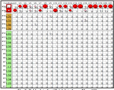
Figure 8 shows a tableplot of all condition indexes and variance decomposition proportions for artificial data, p=20, n=100. According to Figure 8, the top two rows are painted as red for the condition index, the contributions of the variables for the smallest dimensions are seen in this tableplot.
Fig. 6: Tableplot of artificial data for p=15, n=100
Dimensions in the range of 1-14 as green and dimensions in the range of 15-18 as yellow were painted. This means that there is no collinearity problem in the dimensions between 1 to 14. But dimensions between 15-18 should be examined. The collinearity biplot for the smallest two dimensions in Figure 9 account for 0.03% of the total variation. According to Figure 7, the variables of V3,V4,V8,V11,V12,V14,V15 and variables in the range of V17-V21 on Dimension 20 and the variables of V2, V7, V10, V13 on Dimension 19 are effective. Figure 9 supports the comments of Figure 8. The results of both the collinearity biplot and tableplot for artificial data are similar.
Fig. 9: Collinearity biplot of artificial data for p=20, n=100
The Results of Analysis for the Case of Weak Multicollinearity
We used a small simulation data to examine case of weak multicollinearity. One hundred samples were generated from multivariate standard normal distribution with p=5. Figure 10 and 11 present the results of analysis for this small simulation data. Figure 10 indicates a tableplot of condition indexes and variance decomposition proportions for small simulation data. In Figure 10, the top two rows are painted as green for condition indexes. This situation indicates that multicollinearity does not exist and interpretation of Figure 11 has hardly any meaning.
The Results of Analysis for the Case of Strong Multicollinearity
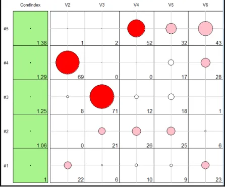
Hald’s Cement Data (Wood et al., 1932) is one classic example of a strong multicollinearity. VIFs for Hald’s Cement Data were obtained as 38.50, 254.42, 46.87, 282.52; condition Indexes (CIs) were obtained as 1, 1.42, 11.98, 1376.88. Tableplot for too high condition index (1376.88) could not be obtained. But the collinearity biplot in Figure 12 were obtained. As a result, use of collinearity biplot in Figure 12 is suggested for visual diagnostics of multicollinearity in case of too high condition indexes.
Fig. 10: Tableplot of weak multicollinearity data, p=5, n=100
Fig. 12: Collinearity biplot for the case of strong multicollinearity, p=4, n=13 4. CONCLUSIONS
In this paper, we have investigated the Tableplot originally suggested by Friendly and Kwan (2009) and biplot which was originally suggested by Gabriel (1971) on one real data and three artificial data. Tableplot and collinearity biplot can be used for visualizing diagnostics of multicollinearity. While both methods seem to give similar results, collinearity biplot is important in terms of determination of outlier observations. While the indicators of multicollinearity data can be seen on the tableplot, in the collinearity biplot, multicollinearity can be detected relatively. But these indicators for the collinearity biplot can be obtained by using linear algebra formulations.
In this study, tableplots were obtained with the libraries of the tableplot, MASS, perturb and car in R program. We have seen that both biplot and the tableplot methods are extremely useful in terms of the direct detection of multicollinearity problem. These two methods are quite useful for high dimensional data. The correct identification of multicollinearity problem in multiple linear models is only possible in the light of all the diagnostics methods. But, the tableplot and the collinearity biplot methods present all information about multicollinearity as a picture. Also, results indicate that Biplot method is preferred to instead of Tableplot for too large condition indexes.
In the future studies, robust tableplot and robust collinearity biplot can be obtained with robust statistical methods and findings may be the compared to conventional methods.
REFERENCES
1. Aitchison, J. and Greenacre, M. (2002). Biplots of Compositional Data. J. Roy. Statist. Soc., Series C. 51(4), 375-392.
2. Andrew, R.W. and Donald, G.W. (1978). Meaningful Multicollinearity Measures. Technometrics, 20(4). 407-412.
3. Belsley, D.A., Kuh, E., and Welsch, R. E. (1980). Regression Diagnostics: Identifying Influential Data and Sources of Collinearity. New York, Wiley.
4. Belsley, D.A. (1991a). A Guide to Using the Collinearity Diagnostics. Computer Science in Economics and Management. 4: 33–50.
5. Belsley, D.A. (1991b). Conditioning Diagnostics: Collinearity and Weak Data in Regression, New York, Wiley.
6. Berk, K.N. (1977). Tolerance and condition in regression computations. J. Amer. Statist. Assoc., 72, 863-866.
7. Chatterjee, S. and Price, B. (1977). Regression Analysis by Example, John Wiley, & Sons, New York.
8. Farrar, D.E. and Glauber, R.R. (1967). Multicollinearity in regression analysis: the problem revisited. Review of Economics and Statistics, 49, 92-107.
9. Fox, J. (1984). Linear Statistical Models and Related Methods, New York, Wiley. 10. Friendly, M. and Kwan, E. (2009). Where's Waldo? Visualizing Collinearity
Diagnostics. Statistical Computing and Graphics. 63(1), 56-65.
11. Gabriel, K.R. (1971). The Biplot Graphic Display of Matrices with Application to Principal Components Analysis. Biometrics, 58, 453-467.
12. Gabriel, K.R. (1978). Least squares approximation of matrices by additive and multiplicative models. J R Statist Soc, Ser. B., 40, 186-196.
13. Gabriel, K.R., and Odoroff, C.L. (1990). Biplots in Biomedical Research. Statistic in Medicine, 9, 469-485.
14. Gower, J.C. and Hand, D.J. (1996). Biplots. London. Chapman & Hall.
15. Hocking, R.R. (1983). Developments in linear regression methodology: 1959-1982, Technometria, 25, 219-249.
16. Jolliffe, I.T. (2002). Principal Component Analysis (2nd ed.). New York: Springer. 17. Kwan, E. (2008). Improving Factor Analysis in Psychology: Innovations Based on the
Null Hypothesis Significance Testing Controversy. Unpublished Ph.D. dissertation, York University, Toronto, Ontario.
18. Marquardt, D.W. (1970). Generalized Inverses, Ridge Regression, Biased Linear Estimation, and Nonlinear Estimation, Technometrics, 12(3), 591-612.
19. Marquardt, D.W. and Snee, R.D. (1975). Ridge regression in practice. The American Statistician, 29, 3-19.
20. Paulson D.S. (2007). Handbook of Regression and Modeling: Applications for the Clinical and Pharmaceutical Industries. Boca Raton, Fla, Chapman and Hall/CRC. 21. R Development Core Team. (2010). R: Language and Environment for Statistical
22. Rawlings, J.O., Pantula, S.G. and Dickey, D.A. (1998). Applied Regression Analysis: A Research Tool, 2nd edition. New York, Springer-Verlag.
23. Silvey, S.D. (1969). Multicollinearity and imprecise estimation. J. Roy. Statist. Soc., 31, 539-552.
24. Theil, H. (1971). Principles of Econometrics. New York, Wiley.
25. Weisberg, S. (1980). Applied Linear Regression. New York, John Wiley & Sons. 26. Wood, H., Steinour, H.H. and Starke, H.R. (1932). Effect of Composition of Portland
cement on Heat Evolved During Hardening. Industrila and Engineering Chemistry, 24, 1207-1214.