EJTIR
ISSN: 1567-7141 http://ejtir.tudelft.nl/
COVID-19 transmission risk minimization at public
transportation stops using Differential Evolution algorithm
Mehmet Metin Mutlu
1Civil Engineering Department, Aydın Adnan Menderes University, Aydın, Turkey.
İlyas Cihan Aksoy
2Civil Engineering Department, Karamanoğlu Mehmetbey University, Karaman, Turkey.
Yalçın Alver
3Civil Engineering Department, Ege University, İzmir, Turkey.
P
ublic transportation vehicles, with their confined spaces and limited ventilation, are considered among the primary factors in the spread of COVID-19. As a measure to slow the spread of the virus during the pandemic, governments have applied passenger capacity restrictions to ensure physical distancing. On the other hand, the increase in the risk of disease transmission associated with passengers waiting together at stops is omitted. In this study, we consider the risk of disease transmission as a travel cost and formulate a risk minimization problem as a transit network frequency setting problem. We develop a bi-level optimization model minimizing the total infection risk occurring at stops, namely, the cumulative disease transmission risk cost. The Differential Evolution algorithm is employed to cope with the NP-hard bi-level transportation network design problem. We propose a novel objective function for the upper-level model, considering the infection risk cost based on passenger traffic at public transportation stops. A congested user-equilibrium transit assignment model is utilized to determine passenger movement. The proposed model is applied to a small-size hypothetical network, and a mid-size test network. Experimental studies provide evidence that the model can produce optimal solutions. Optimization results show significant improvements in the reduction of disease transmission risk compared to the optimizations depending on the traditional practice of transportation network planning based on user and operator costs. The proposed model provides risk cost reductions of 51% and 22% compared to the optimal solutions based on user cost minimization in the hypothetical network and Mandl’s network, respectively.Keywords: coronavirus, COVID-19, Differential Evolution algorithm, public health, public transportation
infection risk, transit frequency design problem.
1 A: Aydın Adnan Menderes University, 09010, Aydin, Turkey T : +90 256 213 75 03 E: [email protected] 2 A: Karamanoğlu Mehmetbey University, 70200, Karaman, Turkey T: +90 338 226 51 71 E: [email protected] 3 A: Ege University, 35040, İzmir, Turkey, T: +90 232 388 60 26 E: [email protected]
1. Introduction
Throughout history, humanity has suffered from contagious diseases, such as the Bubonic Plague and Spanish Flu, which have led to the death of millions of people. On March 11, 2020, the World Health Organization (WHO) identified the recent coronavirus outbreak as a disease on par with the aforementioned by designating it as a global pandemic. As of January 2021, there have been approximately 82 million cases, resulting in approximately 1 810 000 deaths all over the world (WHO, 2021).
One of the leading causes of disease transmission is human interaction, which leads to the rapid spread of the disease, especially in cities with high urban mobility. Extraordinary measures have been taken in many countries during the COVID-19 pandemic to decelerate disease transmission, including limiting public gatherings, implementing transportation restrictions, enforcing social distancing measures, and mandating the closure of businesses and schools, along with comprehensive lockdowns (Bruinen de Bruin et al., 2020).
International, inter-city, and urban travel restrictions have been applied concerning transportation. Many countries have imposed travel bans resulting in the wholesale closure of their borders as a means of preventing the spread of the virus.
Public transportation is likely to induce an increased risk of disease transmission, given that buses and trains are structurally-enclosed spaces where the congregation of large crowds of passengers can pose significant potential for disease transmission. However, such modes of transportation are an essential component of urban mobility particularly for captive riders, especially for commute trips of professionals employed in essential businesses that are exempt from closures during the pandemic such as healthcare, food, and energy. Taking these factors into account, to decrease the risk of disease transmission, passenger space on public transportation is limited to ensure social distancing.
While the reduction of public transportation passenger capacity may lower on-board transmission risk, it also brings with it the consequence of increased passenger wait times, which is accompanied by longer queues at stops. Crowding management is essential to minimize virus spread in all travel stages, including waiting at the stop (Tirachini and Cats, 2020), since crowded stops are likely to increase the infection rates, as physical distancing consequently becomes harder to maintain. Therefore, minimizing the passenger number at stops should be taken into consideration as a precaution in the context of public transportation plans in order to reduce the risk of COVID-19 transmission.
During the pandemic, station crowding can be mitigated by adopting measures such as stop design and demand management measures, including Advanced Transportation Information Systems (ATIS) applications, and encouraging users to change the path choice behavior. Taking precautions pertinent to social distancing, such as changing the stop design or street-queuing, may not be applicable for every stop due to physical limitations. It might not be possible to enlarge the stop areas most of the time, especially in crowded city centers. The utilization of ATIS for demand management and informing the passengers can also be considered as a solution. However, ATIS might not help prevent the virus spread, especially in underdeveloped or developing countries, since all passengers may not own intelligent electronic devices. Like the prementioned measures, changing user behavior may not be possible to be realized in short times. During pandemic circumstances, to provide a safe public transportation system, the precautions regarding the reduction of disease transmission have to be taken immediately. For these reasons, in this study, minimizing disease transmission risk at public transportation stops solely by adjusting headways is thought to be the fastest solution, which can be handled as a transit network frequency setting problem (TNFSP). This method does not require any costs for fleet investments or stop redesign, and the time required for the change of user behavior.
A TNFSP is a sub-problem of a transit network design and frequency setting problem (TNDFSP). Frequency setting is an operational decision and is related to determining the time interval between consecutive departures of transit line vehicles. Frequencies of transit lines are adjusted based on demand in different seasons of a year or periods of a day. This is done to make more efficient use of the public transportation system with respect to operator and user costs. In the same vein, transit line frequency during the pandemic period should be planned with public health as a top priority. In this study, as a means of examining the effect of network design on network users’ reactions (i.e., route choice decisions), and in the interest of calculating infection risk at public transportation stops, we formulated the problem as a bi-level transportation network design problem. The upper-level of the bi-upper-level structure represents the decision-maker, who determines the bus line headways in the network, and the lower-level represents travelers.
Bi-level TNFSPs are NP-hard considering their computational complexity (Magnanti and Wong, 1984), which results in unreasonable computing times for obtaining near-optimal solutions, especially in large networks (Ben-Ayed et al., 1988). Thus, metaheuristic algorithms, which can obtain a near-optimal solution in reasonable times, are used in literature as convenient methods for solving such problems (Farahani et al., 2013).
TNFSPs have been handled many times in literature by considering different objective functions, constraints, and transit assignments.
Yu et al. (2010) tackle the bus frequency design problem by aiming to minimize the total travel time of passengers under the constraint of the fleet size of two operator companies. An iterative approach is applied using a Genetic Algorithm and a label-marking method.
Yoo et al. (2010) address a TNFSP by employing a gradient projection method to maximize the demand on the variable-demand networks by considering the fleet size and frequency constraints. The model proposed by dell’Olio et al. (2012) obtains optimal frequency values and vehicle capacities by minimizing the sum of total user and operator costs via the Hooke-Jeeves Algorithm. Zhao et al. (2015) aim to minimize the sum of total travel time as well as the weighted total number of transfers for transit network users using a Memetic Algorithm in which local search operators were embedded in a Genetic Algorithm.
Verbas and Mahmassani (2015) handle the problem of maximizing wait time savings subject to the constraints of the budget, fleet size, vehicle load, and policy headway by implementing the model on the Chicago Transit Authority network during morning-peak hours.
In the work of Giesen et al. (2016), a multi-objective frequency setting model, which aims to minimize the total user travel time as well as the required fleet size for transit operators, is implemented using the Tabu Search method. The proposed model is performed over a real medium-sized network with two data sets corresponding to morning-peak and off-peak periods. In a recent study, Gholami and Tian (2019) present a comparison of two different frequency determination methods consisting of optimum frequency and demand-based frequency methods. Frequencies are determined for two methods on the routes obtained by Ant Colony Optimization at each iteration.
Finally, in the study of Gkiotsalitis and Cats (2020) regarding social distancing measures in the age of COVID-19, a transit frequency optimization model for metro lines is presented, considering the revenue losses associated with the unaccommodated passenger demand under different social distancing scenarios.
As can be seen in these studies, researches based on TNFSP frequently take user and operator costs into account. To the best of the authors’ knowledge, there is no TNDFSP study considering public health as a transportation cost.
In this study, we propose a bi-level TNFSP model that employs a Differential Evolution Algorithm to minimize infection risk at transit network bus stops with a specific focus on the total cumulative disease transmission risk cost. In the interest of obtaining the total risk cost, congested transit assignment is employed to calculate the number of passengers at stops. The proposed model is tested on a small hypothetical network and Mandl’s test network.
The structure of this article is as follows: Section 2 describes the bi-level optimization model, explaining mathematical models, the objective and constraint functions, the transit assignment method, and the Differential Evolution algorithm. Section 3 presents computational experiments on the test networks, and Section 4 provides conclusions and highlights research gaps to be examined in future studies.
2. Optimization model
2.1 Mathematical model
As the number of people in a crowd and the time that they spend together increases, so too does the risk of infection. To estimate the number of passengers at stops, public transportation trip assignment must be performed. In the model presented in this study, a user-equilibrium type public transportation trip assignment is employed. Although simulations and dynamic assignment models may be considered more suitable for bus stop operation planning, the steady-state assignments are more suitable for bi-level optimization models, considering the computational burden.
In the proposed model, the passenger count of stops with respect to time is obtained using the demand matrix and trip assignment model output. It is assumed that bus stop arrivals are uniform at the first stops of trips. Incoming flows to stops by transfers are calculated based on nominal frequencies, which is the constant frequency value of a line defined by the operator. On the other hand, outgoing flows from the stops are calculated based on congested frequencies. The congested frequency of a line is calculated by the average congested waiting time of passengers in the stops. Average congested waiting time is calculated using the travel cost function presented in the following subsection and differs for each stop and each line.
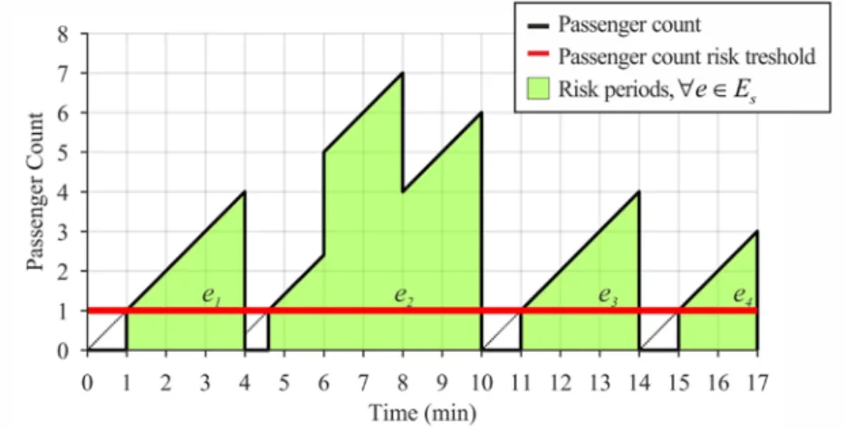
Figure 1. Passenger count, risk threshold, and risk periods in a hypothetical stop
Since trip demand is assumed uniform, passenger number increments at stops caused by starting trips are linear, as can be seen in Figure 1.
In bus stops in particular, social distancing can be maintained up to a certain threshold of passengers. Therefore, disease transmission risk may be considered zero below a given threshold value. Consequently, a threshold parameter for the number of passengers at a stop is employed in the model. As the number of passengers in a stop decreases below the threshold value, the time
passengers spend together is reset to zero. Accordingly, the analysis period is divided into risk periods depending on the threshold value. A graph showing the passenger count, the risk threshold, and the risk periods at a hypothetical stop i is given in Figure 1.
The nomenclature of our optimization model is presented in Table 1. Table 1. Nomenclature
Symbol Meaning
S set of all stops in the transit network. L set of all bus lines in the transit network.
ˆ
A set of route sections. W set of all OD pairs.
ˆ
rs
K set of route section paths between the OD pair rs.
s
E set of risk periods that occurred in the stop s. t time passed in the analysis period.
T duration of the analysis period. t time passed in the risk period.
e
T duration of the risk period e.
( )
s
q t number of passengers at stop s at the time t throughout the analysis period.
( )
s
r t time spent by the passengers at the stop s at risk throughout the analysis period.
( )
s eq t number of passengers at stop s at the time t throughout the risk period e.
( )
s er t time spent by the passengers at the stop s at risk throughout risk period e. ρ ratio of asymptomatic virus carriers in the population.
η risk cost calibration parameter regarding the number of passengers.
𝜁𝜁 risk cost calibration parameter regarding the time passengers spent together. ˆx set of route section flows.
*
ˆx set of route section flows under user-equilibrium constraints. c travel cost function of route sections.
b
n required fleet size.
max b
n maximum allowed fleet size. ˆ
l
f frequency value of line l. min
ˆ
l
f minimum allowed frequency for line l. max
ˆ
l
f maximum allowed frequency for line l. ˆ
l
T roundtrip time of bus line l.
Using the risk threshold value, the function of the passenger count of stops (q t
( )
) and the function of the time that passengers spend together (r t( )
) can be defined numerically, which allows the total cumulative disease transmission risk cost of a transit network to be calculated.Another factor that affects infection risk is the number of infected individuals in a group. During the COVID-19 pandemic, individuals that are identified as being symptomatic carriers are detected and isolated. Asymptomatic carriers, on the other hand, pose the risk of transmission in public life.
Therefore, the parameter representing the ratio of asymptomatic infected individuals, ρ, is employed in the model.
In this study, the aim is to minimize the total cumulative disease transmission risk cost that occurs at bus stops. The objective function adopting mentioned transmission risk factors can be defined as:
(
)
( )( )
( )
0 min 1 1 s T q t s s s S Z=∑∫
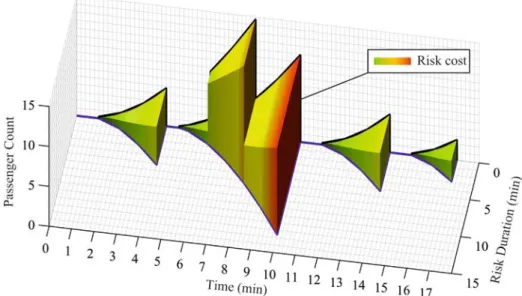
− −ρ ×q t η×r t ζ dt ò (1)where the first operand of multiplication gives the probability that at least one infected individual exists at the stop, the second operand is related to the number of passengers, and the last operand is related to the time that passengers spend together. Exponential parameters η and ζ are employed in the objective function to allow for the calibration of the model by changing the significance of number of passengers and the risk period duration. Objective function components of the hypothetical stop are shown in Figure 2.
Figure 2. Risk duration and passenger count related components of the objective function
The value of the objective function is the multiplication of the components given in Figure 2. Thus, it can be represented by the volume given in Figure 3. Accordingly, the objective function can be calculated using rectangular numerical integration.
By introducing the risk periods to the model, the objective function can be converted into a piecewise function. Consequently, the non-continuous r t
( )
function representing the time spent by the passengers under the infection risk throughout the analysis period is substituted by( )
se s
r t ∀ ∈e E which is defined for each risk period. The objective function then becomes:
(
)
( )( )
( )
0 min 1 1 e s e s T q t s s e e s S e E Z= − −ρ ×q t η×r t ζ dt ∑∑∫
ò ò (2)The risk period duration with respect to time is a linearly-increasing function of time, s
( )
er t =t, where t represents the time passed in the risk period e, at stop s.
The objective function and constraints of the mathematical program are given in Equations 3–7:
(
)
( )( )
0 min 1 1 e s e s T q t s e s S e E Z= − −ρ ×q t η ×t dtζ ∑∑∫
ò ò (3) max 0<nb≤nb (4) min max ˆ ˆ ˆ l l l f ≤ f ≤ f ∀ ∈l L (5)( ) (
)
ˆ * ˆ * ˆ Ω 0 ˆ −ˆ ≥ ∀ ∈ x x x x x c • (6) ˆ ˆ ˆ ˆ ˆ ˆ ˆˆ ˆ ˆ ˆ ˆ , 0 ; 0 , ; Ω ˆ ˆ ˆ ˆ ˆ ˆ ˆ ˆ ; ˆ ˆ δ ∈ ∈ ∈ ≥ ∀ ∈ ≥ ∀ ∈ ∀ ∈ = = ∀ ∈ = ∑
∑ ∑
x rs rs rs a k rs rs rs rs rs a k k a k rs W k K k K x a A X k K rs W X q rs W x X (7)Equation 3 represents the objective function of the problem, which is to minimize the total cumulative disease transmission risk cost at stops.
Equation 4 is the bus fleet constraint, where, nb, the minimum number of required vehicles for
transit operation with the given headway set, is calculated as:
(
)
ceil ˆ ˆ / 06 b l l l L n T f ∈ =∑
× (8)In this study, for the sake of simplicity, return directions of roundtrip bus line routes are not defined. Therefore, round trip times of lines are multiplied by two during fleet size calculation. Equation 5 is a network design constraint for line frequencies, which ensures that the frequencies are between the minimum and the maximum allowed values.
Equation 6 is the lower-level problem constraint that represents the variational inequality formulation for the route section based user-equilibrium transit assignment problem, which determines the route section flows that fulfill the user-equilibrium conditions. Equation 7 represents the non-negativity and the conservation of flow constraints of the user-equilibrium problem.
2.2 Lower-level model
Calculation of the total infection risk to which transit network users are exposed is possible by determining their route choice decisions, which are the output of the lower-level trip assignment model. The trip assignment output is then converted into transit stop count data along the analysis period for each stop in the network in order to calculate the total cumulative disease transmission risk cost.
The lower-level model is a transit assignment model that calculates deterministic user-equilibrium flows under the following assumptions: (1) Passengers do not take disease transmission risk into
account in their route choices. (2) They are assumed to choose the path minimizing their travel cost and board the first arriving bus in the attractive lines set. (3) Transit stops are used as zones where demand originates and terminates. (4) Walking links are not included in the network; therefore, the assignment model does not allow passengers to walk between stops. (5) All bus lines are assumed to have the same in-vehicle travel times while passing through the same itineraries. Bus line segment representation of a transit network is converted into route section representation, and expected travel costs of route sections are calculated using a BPR-like function (Equation 9) as proposed by De Cea and Fernández (1993).
ˆ ˆ ˆ ˆ ˆ ˆ ˆ ˆ ˆ ˆ ˆ ˆ ˆ ˆ ˆ n a a a a a a x x t t a A C f α β + = + + × ∀ ∈ (9)
Where tˆaˆ is the total congested travel cost of the route section ˆa ; taˆ is the in-vehicle travel time on
ˆ
a; fˆaˆ is the sum of frequencies of lines contained in ˆa ;
α
ˆ is the calibration parameter for non-congested waiting time at the stop; xˆaˆ is the passenger flow of ˆa ; xaˆ is the total number ofcompetitive passengers of ˆa , who are the passengers that wait for other route sections that use lines contained in ˆa in the same stop, and the passengers that boarded the lines contained in ˆa at a node before the origin node of ˆa and alighting after; Cˆaˆ is the practical capacity of ˆa , which is the total capacity of the lines contained; ˆn is the calibration parameter for the congested waiting time at a stop.
Route section representation is a proper method for handling common lines problem of transit network design problems. Each route section contains attractive lines that travelers are able to carry out their trips between two nodes. The transit assignment problem can be handled similar to road network assignment using the route section representation. In the route section network, nodes represent bus stops, and the links represent the sets of attractive bus lines traveling between the node pairs. As shown in Figure 4 and Figure 5, the sections of lines 1, 2, and 3 between stops 2 and 3 are grouped in the route section link 4.
The attractive line selection approach, based on minimization of expected travel time, proposed by Chriqui and Robillard (1975), is adopted in the route section generation process of this study. In this study, all lines passing through a road link are assumed to have the same in-vehicle travel time. Therefore, all bus lines passing through the same road link sequence between a node pair are associated to a route section as attractive lines. Slower lines may also be considered attractive after faster lines are congested. Accordingly, separate route sections are generated for the lines using different road links between a node pair even if they have longer in-vehicle travel times. For example, the route section links 5 and 7 between the nodes 2 and 4 are generated as separate links, since the lines 1 and 3 composing the route section link 5 use the road links 2 and 5, whereas line 4 composing the route section link 7 use the road link 3, as represented in Figure 5.
Flows in links (i.e., route sections) containing the same lines, which are presented as competitive flows, result in flow interactions between the links. Therefore, the assignment problem given as a variational inequality in Equation 6 with the constraint set given by Equation 7 has an asymmetric cost function, c
( )
ˆx . Thus, it can be solved using the diagonalization method, which is commonly used for trip assignment problems with asymmetric cost functions due to non-symmetric link flow interactions (Florian and Spiess, 1982; Miandoabchi et al., 2012).Diagonalization is an iterative method that involves fixing the off-diagonal elements of the link cost functions to eliminate link interdependency by fixing all arguments of a link’s cost function other than the link’s own flow to solve a sub-problem in each iteration (Sheffi, 1985).
The sub-problem solved at each iteration of the diagonalization algorithm using Frank and Wolfe (1956) algorithm for the transit assignment problem presented in this study is formulated as:
( ) ˆˆ
(
( ))
ˆ ˆ ˆ ˆ0 min ˆ ,ˆ a x m m a a a A z t ω dω ∈ =∑∫
x (10)where ( )m is the iteration number; ( )ˆ
m a
x is the vector of fixed flow values belonging to the
competitive flow set of the route section ˆa at iteration ( )m .
Following the transit assignment, passenger counts of stops along the analysis period are calculated based on transportation demand between stops, route section frequencies, flows of routes with transfers, and congested waiting times for lines belonging to route sections.
2.3 Upper-level model
An iterative process between the lower-level model and the optimization model is required to determine the optimal frequency set that minimizes the total cumulative disease transmission cost. Due to the complex nature of bi-level transportation network design problems, it is usually not possible to determine the optimal solution in reasonable computing times using exact solution methods, especially in large-scale networks. Therefore, computationally-efficient meta-heuristics are utilized to obtain near-optimal solutions at the expense of solution accuracy (Yang, 2010). In this study, the Differential Evolution algorithm (DE) (Storn and Price, 1997) is employed for solving the proposed frequency setting model due to its strength, simplicity, and robustness in overcoming difficult problems. DE has been used by several researchers in transit network design studies (Zhong et al., 2013; Buba and Lee, 2018).
The steps of DE associated with the proposed frequency setting model are as follows:
Step 0: Initialization. For each agent of the population with size nPop, generate a set of elements
(i.e., frequency set of each line with size nVar), fˆn=
{
fˆn,1,…,fˆn,nVar}
n∈ …{1, , nPop}, with random positions (i.e., frequency values), in search space ( fˆmin< fˆn l, < fˆmax ∀n l, ).Step 1: Calculation. Calculate the fitness values (i.e., the total cumulative disease transmission risk
cost) for each frequency set ˆfn.
Step 1.1: Transit Assignment. Execute the transit assignment for each frequency set ˆfn.
Step 1.2: Passenger Count. Calculate the number of passengers with respect to time at all stops
during the analysis period.
Step 1.3: Risk Calculation. Calculate the cumulative disease transmission risk cost for all stops using
passenger counts.
Step 2: For each frequency set of the current population:
Step 2.1: Mutation. Randomly select three different frequency set indices a, b, and c from the
population; generate the mutated frequency set as ˆ
(
ˆ ˆ)
n= +a F b− c
y f f f where
{
,1, , ,nVar}
n= yn … yn
y and the constant scaling factor F∈
[ ]
0, 2 .Step 2.2: Crossover. Generate a random index r∈
{
1, 2,…, nVar}
and random number Ri∈[ ]
0,1 for each frequency value. Create trial frequency set ˆfn′ as, , , if R CR ˆ or othe ˆ rwise n i i n i n i y i r f f ≤ = ′ = where CR∈
[ ]
0,1 is the crossover probability.Step 2.3: Selection. Calculate the total cumulative disease transmission risk cost values for the trial
frequency sets using the procedure in Step 1. Compare the fitness values of frequency sets to the trial frequency sets and replace the better set for the next generation:
( ) ( )
1 , if ˆ ˆ , otherwi ˆ s ˆ ˆ e i n n n j n j n C C + = ′ ′ ≤ f f f f fStep 3: Termination. Stop if the maximum iteration number is reached and output the best solution;
Otherwise, go to Step 2.
3. Experimental evaluations
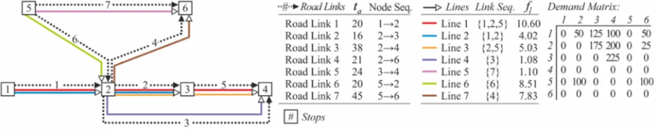
The proposed algorithm is performed on a hypothetical network consisting of six nodes, seven links, and seven transit lines. The hypothetical network built allows observation of a network with common lines, route shifts due to congestion, and stops that cause the number of waiting passengers to increase rapidly due to transfer routes. Bus line segments, link sequences and frequencies ( ˆ
l
f ), stops and demand between stops, road links, and road link travel times (ta) that
correspond to in-vehicle travel times of associated bus lines are illustrated in Figure 4. Line frequencies given in this figure are obtained from another model performed on the same network, which optimizes frequencies for user and operator cost minimization.
Figure 4. Bus line segment representation of the public transportation network
In every iteration of the proposed optimization model, the bus line segment network is converted to a route section network, and route section frequencies and capacities are calculated. The route section network, frequency values, and capacity values are given in Figure 5.
Figure 5. Route section representation and characteristics of the network
Algorithms were coded using MATLAB R2017a and carried out on a 64-bit computer with an Intel(R) Core(TM) i7 2.60 GHz CPU and 16 GB RAM. The average duration of an optimization terminated at the 100th iteration is 12 minutes for the network above.
In this work, the bus fleet size, max b
n , is assumed 50 buses. For all lines, bus capacities are 30 passengers, maximum and minimum allowed frequencies are 1 and 60 runs/hour, respectively. Transit assignment cost function parameters are set as ˆ 0.50α = , β =ˆ 1.00, and nˆ=4.00. Parameters
used for calculating total cumulative disease transmission risk based on passenger counts are 0.20
ρ= , η =2.00, and ζ =1.50. The passenger count risk threshold is set to 3 for all stops. As for the parameter values of DE, Storn and Price (1997) state that it is logical to choose a value between nVar×5 and nVar×10 for nPop. Therefore, nPop is defined 50. The number of iterations to terminate the algorithm, determined by a trial and error approach, is set 100. To better show the effect of different parameter values on the solution quality, F and CR values are selected from the sets F={0.5, 1, 1.5, 2}, CR={0.2, 0.4, 0.6, 0.8}. We execute three replications for each of 16 combinations of parameters, resulting in 48 optimizations with 100 iterations of 50 population. Table 2 presents the average risk costs for all parameter combinations, showing clearly that the best solutions are obtained in the combination of F=0.5 and CR=0.8, with the average risk cost of 91 296.
Table 2. Comparative results of all parameter combinations
Cumulative Transmission Risk Cost Values
F=0.5 F=1 F=1.5 F=2
CR=0.2 97 886 121 063 187 124 240 597 CR=0.4 91 316 125 610 279 383 254 596 CR=0.6 128 629 167 255 323 592 485 635 CR=0.8 91 296 146 306 533 251 1 370 728
The proposed algorithm with F=0.5 and CR=0.8 is executed for 30 independent runs to demonstrate the algorithm’s stability. Frequency values for the best and worst solutions, average value, standard deviation, and coefficient of variation values for the risk costs of 30 optimization runs are presented in Table 3.
Table 3. Risk minimization results obtained by the proposed model
Total Risk Cost *
Line Frequency Values (runs/hour)
1 2 3 4 5 6 7
Best 58 872 10.60 4.02 5.03 1.08 1.10 8.51 7.83 Worst 112 834 10.94 3.16 5.15 1.00 1.33 7.43 10.20 * Average = 87 594, Standard Deviation = 13 765, Coefficient of Variation = 12%
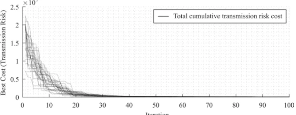
We experienced that minor changes in solution sets lead to significant changes in total cost. Therefore, the coefficient of variation value of 12% can be considered acceptable. Figure 6 depicts the convergence process for all independent runs along 100 iterations. It can be seen that in all runs, the algorithm converges in about 50 iterations.
The proposed risk minimization model is modified with objective functions given in Equations 11 and 12 are performed on the same network to obtain the user-optimal and user & operator-optimal frequency sets. ˆ ˆ ˆ ˆ ˆ ˆ min U a a a A z t x ∈ =
∑
× (11) ˆ & ˆ ˆ ˆ ˆ ˆ ˆ ˆ min U O a a OW l l l L a A z t x T f ∈ ∈ =∑
× + ×∑
× (12)where OW is the weight of operator cost.
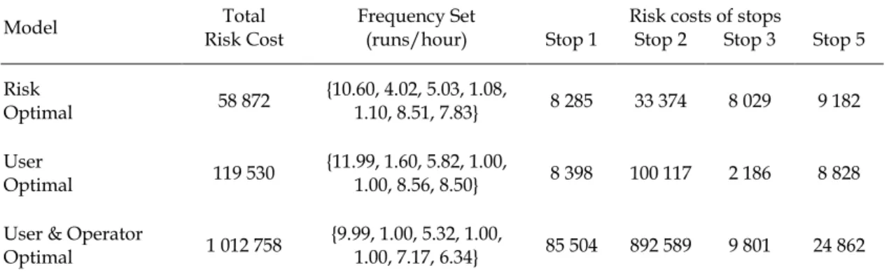
Optimization results of the best solutions of risk-optimal, user-optimal, and user & operator-optimal models are given in Table 4.
Table 4. Results of optimization models performed on the network
Model Risk Cost Total Frequency Set (runs/hour) Stop 1 Risk costs of stops Stop 2 Stop 3 Stop 5 Risk
Optimal 58 872 {10.60, 4.02, 5.03, 1.08, 1.10, 8.51, 7.83} 8 285 33 374 8 029 9 182 User
Optimal 119 530 {11.99, 1.60, 5.82, 1.00, 1.00, 8.56, 8.50} 8 398 100 117 2 186 8 828 User & Operator
Optimal 1 012 758 {9.99, 1.00, 5.32, 1.00, 1.00, 7.17, 6.34} 85 504 892 589 9 801 24 862
As a result of experimental studies, we found that minor changes in frequency values lead to enormous differences in risk cost. The minimum total risk cost is achieved in the risk minimization model proposed in this study, as expected. The risk cost reductions compared to user-optimal and user & operator-optimal solutions are 51% and 94%, respectively. The reason for the great differences in total risk costs between different models is the specific topological design of the hypothetical network and the demand matrix, which are generated to emphasize the effect of employing different optimization objectives. Stops 4 and 6 have no trip demand and are not used for transfers. Consequently, the risk cost is calculated zero for these stops.
Figure 7. Passenger count at Stop 2 between the 15th and 45th minutes of the analysis period In Figure 7, the passenger counts at Stop 2, the stop with the most passenger traffic, are given to attain the best solutions for three performed models. It can be seen that the risk-optimal model proposed in this study ensures that the number of passengers drops below the risk threshold more
frequently, and the stop is less crowded. Therefore, passengers spend less time together, resulting in less exposure to infection risk.
The proposed model allows for incorporating the differences in space between individual stops by setting different threshold values to each stop since the stop capacities may vary. Table 5 shows the risk costs resulting from the frequency sets obtained by the risk-optimal model for five different threshold sets. The threshold values of Stop 1 and 2 are increased to 10 passengers in turn in the stop passenger threshold sets 2 and 3 for the sake of comparison. The threshold sets 4 and 5 are generated randomly to demonstrate that the model is capable of handling individual threshold values of stops.
Table 5. Risk costs for different threshold sets
Threshold
Set Risk Cost Total
Threshold Values (Risk Cost)
Frequency Set (runs/hour) Stop 1 Stop 2 Stop 3 Stop 5
1 58 872 3 (8 285) 3 (33 374) 3 (8 029) 3 (9 182) {10.60, 4.02, 5.03, 1.08, 1.10, 8.51, 7.83} 2 45 303 10 (1 431) 3 (33 829) 3 (4 698) 3 (5 343) {9.84, 3.00, 6.63, 1.27, 1.25, 9.39, 7.51} 3 30 228 3 (4 689) 10 (12 126) 3 (5 976) 3 (7 436) {11.98, 3.28, 4.19, 1.11, 1.00, 8.86, 8.18} 4 16 821 5 (3 173) 10 (6 660) 2 (2 848) 4 (4 139) {12.76, 1.00, 5.09, 1.00, 1.32, 9.39, 5.68} 5 74 887 7 (4 414) 2 (68 282) 9 (408) 8(1 781) {8.33, 4.97, 8.03, 1.56, 1.00, 8.64, 8.34} In threshold set 2, the threshold value of Stop 1 is higher. Therefore, the gathering of more passengers is acceptable in terms of disease transmission risk. As a result, the optimization conducted using threshold set 2, compared to the threshold set 1, yields to lower frequency values of lines 1 and 2, which have routes originating from Stop 1. The frequency values of lines obtained using threshold set 3 are not possible to analyze since six of the total seven lines originate, terminate, or pass through stop 2, and the total risk cost depends on all stops that these lines are related. On the other hand, the risk cost is reduced due to the high threshold value since Stop 2 is the stop with the most passenger traffic in the network.
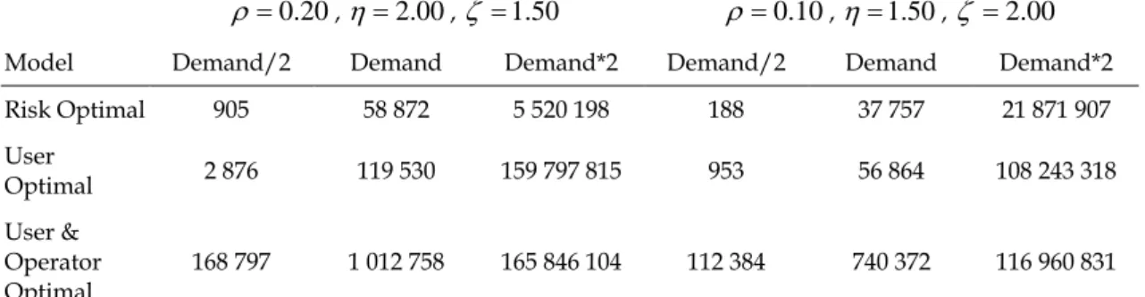
The variations of demand and the parameter values used to calculate the risk cost are expected to affect the risk cost. In order to demonstrate such an effect, optimal frequency sets of three different optimality concerns are obtained for two sets of parameter values and three different demand cases, as shown in Table 6.
Table 6. Risk costs under the different demand values and transmission risk cost function parameter values
0.20
ρ= , η=2.00, ζ =1.50 ρ=0.10, η=1.50, ζ =2.00 Model Demand/2 Demand Demand*2 Demand/2 Demand Demand*2 Risk Optimal 905 58 872 5 520 198 188 37 757 21 871 907 User Optimal 2 876 119 530 159 797 815 953 56 864 108 243 318 User & Operator Optimal 168 797 1 012 758 165 846 104 112 384 740 372 116 960 831
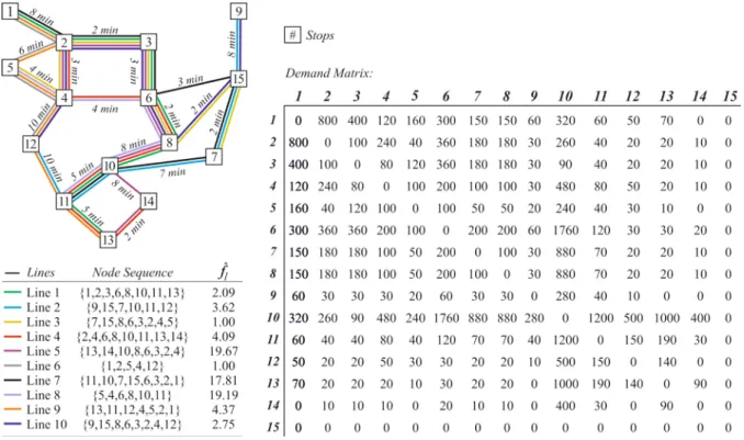
In addition to the small-size hypothetical network, we apply the proposed model to Mandl’s network (Mandl, 1980) consisting of 15 nodes, 21 bi-directional links to test its applicability in terms of computational time.
Figure 8. Mandl’s network with 10 routes
The route set of the best solution for the 10-route network in the study of Arbex and da Cunha (2015) is used in this network to optimize the frequencies for disease transmission risk minimization. The link travel times, bus route details, and the demand matrix are presented in Figure 8. It should be noted that all lines operate through the node sequence forth and back to complete a run. Risk costs calculated using the frequency sets determined by risk-optimal, user-optimal, and user & operator-optimal models are given in Table 7. All parameter values of DE, transit assignment model, and risk calculation is set as in the hypothetical network except for max
b
n and bus capacity. max
b
n and bus capacity are set to 75 and 50 in this case, respectively. A run with 100 iterations of 50 populations in Mandl’s Network takes a processing time of 1.5 hours approximately.
Table 7. Results of optimization models performed on the 10-route Mandl’s Network.
Model Risk Cost Total Line Frequency Values (runs/hour)
1 2 3 4 5 6 7 8 9 10 Risk Optimal 50 934 945 2.09 3.62 1.00 4.09 19.67 1.00 17.81 19.19 4.37 2.75 User Optimal 65 002 557 17.87 9.29 1.00 1.00 8.50 1.00 13.45 21.63 1.00 1.00 User & Operator Optimal 72 960 539 17.06 8.43 1.00 4.21 8.89 1.03 11.97 16.67 1.00 1.70
As can be seen in Table 7, the risk cost minimization model leads to a 22% and 30% reduction in the risk cost compared to user-optimal and user & operator-optimal solutions, respectively. The results show that the risk optimization model yields smaller risk cost differences in a more realistic network compared to the hypothetical network.
4. Conclusions and future research
In this paper, we have developed a transit frequency setting model that aims to provide a solution that promotes disease transmission risk minimization at public transportation stops during the COVID-19 pandemic. The main contribution of the paper lies in proposing a new transit frequency design problem with the inclusion of a novel objective function that takes into account the infection risk based on passenger movement at public transportation stops.
The proposed model is formulated as a bi-level TNFSP with a congested transit assignment model in the lower level. DE is employed to overcome the inherent complexity of the problem. The computational experiments demonstrate that the proposed model can yield optimal solutions. The optimization results demonstrate significant improvements in disease transmission risk reduction performance when compared to the traditional practice of network planning based on user and operator costs.
Decision-makers and planners can utilize the model developed in this study as a decision support tool for decreasing the risk of the virus spread by means of transit frequency setting, without the requirement of investment for an ATIS infrastructure and construction to redesign the stops. Since the model takes the available bus fleet size into consideration as a constraint, there will also be no requirement for an investment to increase the fleet size. For developed countries, investment cost may not be a significant limitation in exceptional circumstances such as a pandemic. For this reason, to reduce the number of passengers waiting at the stops, precautions such as stop redesign and street-queuing can be taken. However, all stops may not be suitable for these types of precautions due to physical limitations. In the cases of both partially or fully improved transit systems in terms of stop crowding, the proposed model is applicable through the stop risk threshold parameter, which can be set individually for each stop.
Finally, we introduce the following suggestions for consideration in future research to improve the proposed model.
In this study, a steady-state assignment model is employed in the lower-level model, and the risk is calculated in a stop-based manner. To make a more accurate (though not necessarily safer) passenger-based risk calculation, characterized by more detailed passenger traffic information at public transportation stops, dynamic assignment or simulation models can be considered for the lower-level model. The lower-level model is executed through numerous repetitions of the upper-level iterations. Since dynamic assignment and simulation models require longer computation durations, the problem should be evaluated with the replaced lower-level model, taking computational performance into account.
Congestion is considered for transit route choice of passengers in this study, while bus capacities are assumed restricted to assure adequate in-vehicle physical distance. It is also assumed that the pandemic condition does not affect the passenger route choice behavior and that passengers choose a path minimizing their total travel costs. However, the long-term route choice behaviors of passengers are likely to change in a way that they perceive transmission risk due to busy buses or stops as a component of generalized travel cost. Hence, in future studies, infection risk occurring due to in-vehicle congestion and crowding at the stops can also be considered in the transit assignment model.
Acknowledgments
The authors would like to thank the editor and two anonymous reviewers for their insightful and constructive comments that contributed to improve this paper. The authors would also like to thank EGE-PİK and Ege University Directorate of Library and Documentation for proofreading the article.
References
Arbex, R. O. and da Cunha, C. B. (2015). Efficient transit network design and frequencies setting multi-objective optimization by alternating multi-objective genetic algorithm. Transportation Research Part B: Methodological, 81(April 2016), 355–376.
Ben-Ayed, O., Boyce, D. E. and Blair, C. E. (1988). A general bilevel linear programming formulation of the network design problem. Transportation Research Part B, 22(4), 311–318.
Bruinen de Bruin, Y., Lequarre, A.-S., McCourt, J., Clevestig, P., Pigazzani, F., Zare Jeddi, M., Colosio, C. and Goulart, M. (2020). Initial impacts of global risk mitigation measures taken during the combatting of the COVID-19 pandemic. Safety Science, 128(2020), 104773.
Buba, A. T. and Lee, L. S. (2018). A differential evolution for simultaneous transit network design and frequency setting problem. Expert Systems with Applications, 106, 277–289.
Chriqui, C. and Robillard, P. (1975). Common Bus Lines. Transportation Science, 9(2), 115.
De Cea, J. and Fernández, E. (1993). Transit Assignment for Congested Public Transport Systems: An Equilibrium Model. Transportation Science, 27(2), 133–147.
dell’Olio, L., Ibeas, A. and Ruisánchez, F. (2012). Optimizing bus-size and headway in transit networks. Transportation, 39(2), 449–464.
Farahani, R. Z., Miandoabchi, E., Szeto, W. Y. and Rashidi, H. (2013). A review of urban transportation network design problems. European Journal of Operational Research, 229(2), 281–302.
Florian, M. and Spiess, H. (1982). The convergence of diagonalization algorithms for asymmetric network equilibrium problems. Transportation Research Part B: Methodological, 16(6), 477–483.
Frank, M. and Wolfe, P. (1956). An algorithm for quadratic programming. Naval Research Logistics Quarterly, 3(1‐2), 95 –110.
Gholami, A. and Tian, Z. (2019). The comparison of optimum frequency and demand based frequency for designing transit networks. Case Studies on Transport Policy, 7(4), 698–707.
Giesen, R., Martínez, H., Mauttone, A. and Urquhart, M. E. (2016). A method for solving the multi‐ objective transit frequency optimization problem. Journal of Advanced Transportation, 50(8), 2323–2337. Gkiotsalitis, K. and Cats, O. (2020). Optimal frequency setting of metro services in the age of COVID-19 distancing measures. arXiv preprint, arXiv:2006.05688.
Magnanti, T. L. and Wong, R. T. (1984). Network Design and Transportation Planning: Models and Algorithms. Transportation Science, 18(1), 1–55.
Mandl, C. E. (1980). Evaluation and optimization of urban public transportation networks. European Journal of Operational Research, 5(6), 396–404.
Miandoabchi, E., Farahani, R. Z. and Szeto, W. Y. (2012). Bi-objective bimodal urban road network design using hybrid metaheuristics. Central European Journal of Operations Research, 20(4), 583–621. Sheffi, Y. (1985). Urban transportation networks. Prentice-Hall, Englewood Cliffs, NJ.
Storn, R. and Price, K. (1997). Differential Evolution – A Simple and Efficient Heuristic for global Optimization over Continuous Spaces. Journal of Global Optimization, 11, 341–359.
Tirachini, A. and Cats, O. (2020). COVID-19 and Public Transportation: Current Assessment, Prospects, and Research Needs. Journal of Public Transportation, 22(1), 1–34.
Verbas, İ. Ö. and Mahmassani, H. S. (2015). Integrated Frequency Allocation and User Assignment in Multimodal Transit Networks. Transportation Research Record: Journal of the Transportation Research Board, 2498(April), 37–45.
WHO (2021). Coronavirus Disease (COVID-19) Dashboard. World Health Organization, viewed 2 January 2021, <https://covid19.who.int/>.
Yang, X.-S. (2010). Engineering Optimization. Operational Research Quarterly (1970-1977). Hoboken, NJ, USA: John Wiley & Sons, Inc.
Yoo, G. S., Kim, D. K. and Chon, K. S. (2010). Frequency design in urban transit networks with variable demand: Model and algorithm. KSCE Journal of Civil Engineering, 14(3), 403–411.
Yu, B., Yang, Z. and Yao, J. (2010). Genetic Algorithm for Bus Frequency Optimization. Journal of Transportation Engineering, 136(6), 576–583.
Zhao, H., Xu, W. (Ato) and Jiang, R. (2015). The Memetic algorithm for the optimization of urban transit network. Expert Systems with Applications, 42(7), 3760–3773.
Zhong, J.-H., Shen, M., Zhang, J., Chung, H.S.-H., Shi, Y.-H. and Li, Y. (2013). A Differential Evolution Algorithm With Dual Populations for Solving Periodic Railway Timetable Scheduling Problem. IEEE Transactions on Evolutionary Computation, 17(4), 512–527.