Selçuk J. Appl. Math. Selçuk Journal of Vol. 13. No. 2. pp. 11-24, 2012 Applied Mathematics
A Trivariate F Distribution of Markov Dependent F Distributed Random Variables
Funda ·I¸sçio¼glu, Muhammet Bekçi
Department of Statistics, Faculty of Science, Ege University, 35100, Bornova, Izmir, Turkiye
e-mail:funda.akdere@ ege.edu.tr,muham m et.b ekci@ ege.edu.tr
Received Date: October 19, 2011 Accepted Date: December 11, 2012
Abstract. The trivariate F distribution comes out with the ratios of the chi-squared random variables. In its classical form it has marginals on …xed de-nominator and arbitrary numerator degrees of freedom parameters. However it was reduced to have marginals on …xed (or arbitrary) numerator but arbitrary denominator degrees of freedom parameters in the literature. In this paper we introduce a new form which has marginals on both arbitrary numerator and de-nominator but in the case of Markov dependent random variables. We represent the distribution of those random variables and by means of the joint probability density function we study the bivariate, univariate and conditional distribu-tions. Also some graphics and numerical results for the correlation between the random variables are given.
Key words: Multivariate F distribution; Markov dependency; Probability den-sity function; Moment; Correlation coe¢ cient.
2000 Mathematics Subject Classi…cation: 62H10. 1. Introduction
In the case of classical bivariate F distribution [1, 2] when the ratios of two chi-squared random variables (rv s) are taken into consideration, the related univariate F marginal distributions have one degree of freedom (df ) parameter in common. When a multivariate F distribution is considered, all the marginal distributions of the this usual multivariate kind are also F distributions with an arbitrary numerator and a common (…xed) denominator df. The rv with a common df on the denominator provides a positive correlation into the distrib-ution. Jones [3] introduced two new distributions, a multivariate t distribution and a multivariate beta distribution which had a natural relationship to the
standart multivariate F distribution. Jones [4] also studied a dependent bivari-ate t distribution with marginals on di¤erent df. Olkin and Liu [5] presented the same bivariate beta distribution as in [3] but derived in a di¤erent way and studied its dependency properties. Al-Zahim and El-Bassiouny [6] took into consideration the bivariate F distribution with marginals on …xed numerator but an arbitrary denominator df and also presented a multivariate beta density which was related to their multivariate F distribution. Unlike these studies El-Bassiouny and Jones [7] provided an alternative bivariate F distribution with F marginals, each with its own arbitrary numerator and denominator df by adding a new chi-squared rv independent of the other rv s to the denominator. This study eliminated the disadvantage of the distribution whose univariate F marginals have the same denominator or numerator df.
In this paper we provide a new alternative multivariate F distribution with all its F marginals considered with Markov dependency structure and each with its own arbitrary numerator and denominator df parameters. To this end let us consider the following rv s;
(1) F1= X1=v1 X0=v0 ; F2= X2=v2 X1=v1 ; F3= X3=v3 X2=v2 ; :::; Fm= Xm=vm Xm 1=vm 1
We considered the case m = 3 for simplicity, obtained some important distri-bution properties [8,9] of a trivariate F distridistri-bution and its related bivariate and univariate F distributions. The proposed trivariate F distribution with the marginal F distributions on arbitrary numerator and denominator df such as fv1; v0g; fv2; v1g and fv3; v2g; is de…ned as the joint distribution of
(2) F1= X1=v1 X0=v0 ; F2= X2=v2 X1=v1 ; F3= X3=v3 X2=v2
We …rstly derived the joint probability density function (pdf ) of the rv s given in (2), illustrated its shape graphically and gave its product moment in Section 2. Then in Section 3 we obtained the bivariate distributions of those rv s in (2) considering all the pairs. Their joint pdf s and moments were given. Also the correlation coe¢ cients of those rv s were represented. The univariate case, the conditional distributions and moments were derived in Sections 4 and 5 respectively. In the end of Section 6 the multivariate case was given.
2. Trivariate F Distribution
(3) g(f1; f2; f3) = C123 fv1+v2+v32 1 1 f v2+v3 2 1 2 f v3 2 1 3 (1 +v1 v0f1+ v2 v0f1f2+ v3 v0f1f2f3) n123; f1; f2; f3> 0; where C123= (n123)(vv10) v1 2 (v2 v0) v2 2(v3 v0) v3 2 (v0 2) ( v1 2) ( v2 2) ( v3 2) ; n123= v0+ v1+ v2+ v3 2
and (:) is the Gamma function.
Proof. For F1=XX10=v=v10; F2= XX12=v=v21; F3= XX32=v=v32 , in order to get the joint pdf of F1; F2 and F3 we use the following transformations, x0 = f4; x1 = (v1=v0)f1f4; x2 = (v2=v0)f1f2f4; x3 = (v3=v0)f1f2f3f4 and hence the jacobian is (v1v2v3=v03)f12f2f43. Since the rv s X0, X1, X2and X3are independent and have a chi-square distribution with the v0, v1, v2 and v3 df s respectively, we can write the joint pdf as follows,
g(f1; f2; f3; f4) = 2 v02 (v0 2) fv02 1 4 e f4 2 2 v1 2 (v1 2) (v1 v0 f1f4) v1 2 1e 1 2(v1v0f1f4) 2 v22 (v2 2) (v2 v0 f1f2f4) v2 2 1e 1 2(v2v0f1f2f4) (4) 2 v3 2 (v3 2) (v3 v0 f1f2f3f4) v3 2 1e 1 2(v3v0f1f2f3f4) v1v2v3 v3 0 f12f2f43
Then we integrate (4) over f4from 0 to 1 , it follows
g(f1; f2; f3) = 2 n123v v1 2 1 v v2 2 2 v v3 2 3 (v0 2) ( v1 2) ( v2 2) ( v3 2) fv1+v2+v32 1 1 f v2+v3 2 1 2 f v3 2 1 3 (5) 1 Z 0 fn123 1 4 e (v1f12v0+v2f1f22v0 +v3f1f2f32v0 +1 2)f4 df4 De…ne I =R1 0 fn123 1 4 e (v1f12v0+v2f1f22v0 +v3f1f2f32v0 +1 2)f4
df4 for the integral over f4 in (5), and by using the property of the Gamma function I can be simpli…ed to
= v1f1 2v0 +v2f1f2 2v0 +v3f1f2f3 2v0 +1 2 n123 (n123)
Thus the proof follows substituting the result of I in (5) and making the re-maining manipulations.
2.1. Product Moments
Theorem 2.2. Let r1, r2 and r3 be nonnegative such that r1 v20, r2 v21 + r1 and r3 v22 + r2 then E(Fr1 1 F2r2F3r3) = v0 v1 r1 v1 v2 r2 v2 v3 r3 v0 2 r1 v1 2 + r1 r2 v0 2 v1 2 (6) v2 2 + r2 r3 v3 2 + r3 v2 2 v3 2
Proof.From the de…nition of F1, F2 and F3 in (2) , we can write
E(Fr1 1 F r2 2 F r3 3 ) = v0 v1 r1 v1 v2 r2 v2 v3 r3 E(Xr1 r2 1 )E(X r1 0 )E(X r2 r3 2 )E(X r3 3 ) It is known that ( see, Johnson et al [9]), if Yi 2(ni); then for some non-negative integers ri; i = 1; 2; :::; m we have E(Yiri) =
2ri (ni2+ri) (ni2) ; by using this de…nition we get E(Fr1 1 F r2 2 F r3 3 ) = v0 v1 r1 v1 v2 r2 v2 v3 r3 2r1 r2 v1 2 + r1 r2 v1 2 2 r1 v0 2 r1 v0 2 2r2 r3 v2 2 + r2 r3 v2 2 2r3 v3 2 + r3 v3 2
and the proof is completed by some simpli…cations. 3. Bivariate F Distributions
Theorem 3.1. The joint pdf of F1 and F2in (2) is given by
(7) g(f1; f2) = C1;2 fv1+v22 1 1 f v2 2 1 2 (v1f1 v0 + v2f1f2 v0 + 1) n12 ; f1; f2> 0;
where C1;2 = (n12)(vv10) v1 2 (v2 v0) v2 2 v0 2 v1 2 v2 2 ; n12= v0+ v1+ v2 2 .
Proof. This proof is similar with the proof of Theorem 2.1, we just take F1 = XX10=v=v10; F2 = XX21=v=v21; and do similar transformations. Also if we integrate the trivariate pdf found in (3) over f3from 0 to 1, we also get the joint pdf of F1 and F2:
The joint pdf s and counter plots of F1 and F2 for di¤erent values of v0; v1 and v2 are given in Figure 1.
Theorem 3.2. The joint pdf of F1, F3(F1and F3are independent rv s) de…ned in (2) is given as (8) g(f1; f3) = C1;3 fv12 1 1 f v3 2 1 3 (1 +v1 v0f1) v0+v1 2 (1 + v3 v2f3) v2+v3 2 ; f1; f3> 0; where C1;3= (v1 v0) v1 2 (v3 v2) v3 2 B v0 2; v1 2 B v2 2; v3 2 ; and B(:; :) is the Beta function.
Proof. If we integrate (3) over f2from 0 to 1, we can get the joint pdf of F1 and F3 . g(f1; f3) = C123 1 Z 0 fv1+v2+v32 1 1 f v2+v3 2 1 2 f v3 2 1 3 (1 + v1 v0f1+ v2 v0f1f2+ v3 v0f1f2f3) n123df3 where C123= (n123)(vv10) v1 2 (v2 v0) v2 2(v3 v0) v3 2 (v0 2) ( v1 2) ( v2 2) ( v3 2) ; n123= v0+ v1+ v2+ v3 2
and (:) is the Gamma function. De…ne 1 + v1f1
v0 = a and then f2 =
v0a
v2f1+v3f1f3tan
2 and hence df2= v2f12v+v03af1f3tan (cos12 )d then we get
g(f1; f3) = 2A
2
Z
0
where A = C123a n123f v1+v2+v3 2 1 1 f3 v3 2 1( v0a v2f1+v3f1f3) v2+v3
2 and by means of the
Lemma 4.1 and making some simpli…cations we get the joint pdf of F1 and F3. 3.1. Product Moments and Correlations
Theorem 3.3. Let r1; r2; r3; r4; r5 and r6 be nonnegative such that r1 v20; r2 v21 + r1; r3 v21; r4 v22 + r3; r5 v20 and r6 v22 then (9) E(Fr1 1 F2r2) = ( v0 v1 )r1(v1 v2 )r2 v0 2 r1 v21+ r1 r2 v22 + r2 v0 2 v1 2 v2 2 E(Fr3 2 F r4 3 ) = ( v1 v2 )r3(v2 v3 )r4 v1 2 r3 v2 2 + r3 r4 v3 2 + r4 v1 2 v2 2 v3 2 E(Fr5 1 F3r6) = E(F1r5)E(F3r6) = (v0 v1 )r5(v2 v3 )r6 v0 2 r5 v1 2 + r5 v2 2 r6 v3 2 + r6 v0 2 v1 2 v2 2 v3 2
Proof. By means of the de…nitions of F1, F2 and F3 in (2) the proof was completed in the same way as in the proof of Theorem 2.2.
Corollary 3.1. The correlation coe¢ cient between F1 and F2 is;
F1;F2 = 1 q v1(v0+v1 2)(v1+v2 2) v2(v0 4)(v1 4) ; vi> 4; i = 0; 1 .
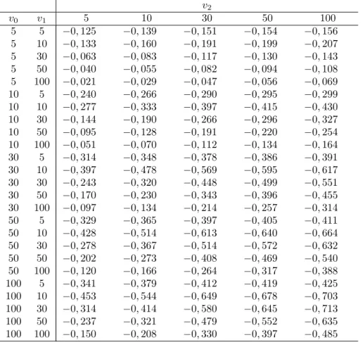
We also present Table 2 to give numerical illustration of the correlation coe¢ -cient between these two rv s.
Proof. Let r1 = 0 and r2 = 1; r1 = 1 and r2 = 0; and r1 = r2 = 1 in (9) respectively , we get the following moments and product moments,
(10) E(F1) = v0 v0 2 ; v0> 2 (11) E(F2) = v1 v1 2 ; v1> 2 (12) E(F1F2) = v0 v0 2 ; v0> 2
and let U and V have 2 distributions with v
1 and v2 df, then X = U=vV =v21 is F distributed with v1 and v2 df. In this case the variance of the rv X is ( v2
v2 2)
2 2 v1(
v1+v2 2
v2 4 ) then through this property we can write
(13) V ar(F1) = 2v2 0(v0+ v1 2) v1(v0 2)2(v0 4) ; v0> 4 (14) V ar(F2) = 2v2 1(v1+ v2 2) v2(v1 2)2(v1 4) ; v1> 4 then by (10)-(12) we write the covariance,
(15) Cov(F1; F2) = E(F1F2) E(F1)E(F2) =
2v0 (v0 2)(v1 2)
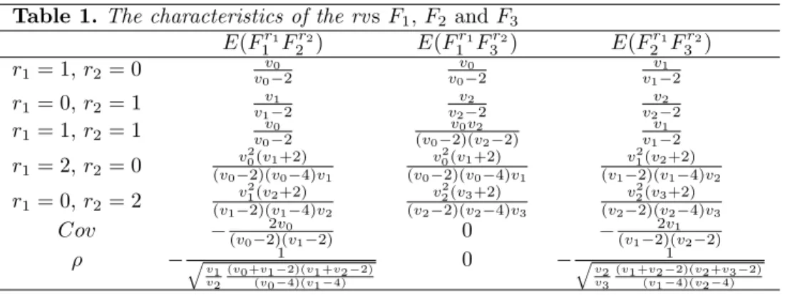
and by (13)-(15) we obtain the correlation coe¢ cient. We present the covari-ances and the correlation coe¢ cients of F1, F2and F3with their related product moments in the following Table 1.
Table 1.The characteristics of the rv s F1; F2 and F3 E(Fr1 1 F2r2) E(F1r1F3r2) E(F2r1F3r2) r1= 1; r2= 0 v0v02 v0v02 v1v12 r1= 0; r2= 1 v1v12 v2v22 v2v22 r1= 1; r2= 1 v0v02 (v0 v2)(v0v22 2) v1v12 r1= 2; r2= 0 v 2 0(v1+2) (v0 2)(v0 4)v1 v02(v1+2) (v0 2)(v0 4)v1 v21(v2+2) (v1 2)(v1 4)v2 r1= 0; r2= 2 v 2 1(v2+2) (v1 2)(v1 4)v2 v2 2(v3+2) (v2 2)(v2 4)v3 v2 2(v3+2) (v2 2)(v2 4)v3 Cov 2v0 (v0 2)(v1 2) 0 2v1 (v1 2)(v2 2) 1 q v1 v2(v0+v1 2)(v1+v2 2)(v0 4)(v1 4) 0 q 1 v2 v3(v1+v2 2)(v2+v3 2)(v1 4)(v2 4)
4. Univariate F Distributions and Their Moments
The following Lemma can be used in order to derive the marginal pdf of F1; F2 and F3 and in some other derivations throughout the article.
Lemma 4.1. The following identity is given in [10].
2
Z
0
sinax cosbxp1 k2sin2xdx =1 2B( a + 1 2 ; b + 1 2 )F ( a + b 2 ; 1 2; a + b + 2 2 ; k 2)
with a > 1; b > 1; jkj < 1; where B(a+12 ;b+12 ) is the Beta function and F (a+b 2 ; 1 2; a+b+2 2 ; k
2) is the Gauss hypergeometric function.
The univariate marginal pdf s of F1, F2 and F3 are known as F-distribution and can be given in the compact form as below
(16) g(fk) = vk vk 1 vk 2 B vk 1 2 ; vk 2 f vk 2 1 k 1 + vk vk 1 fk vk 1+vk 2 ; fk> 0 ; k = 1; 2; 3 .
Theorem 4.1Let rk (k = 1; 2; 3) be nonnegative such that rk vk21, then
(17) E (Frk k ) = vk vk 1 rk vk 2 + rk vk 1 2 rk vk 1 2 vk 2
This theorem gives the rth moments of F-distributed random variables with di¤erent degrees of freedoms. For the rth moment of F-distribution we can refer to [11].
Proof. By using (16) we obtain the rkth moment of the rv Fk as follows
E (Frk k ) = vk vk 1 vk 2 B vk 1 2 ; vk 2 1 Z 0 frk k f vk 2 1 k (1 + vk vk 1 fk) vk 1+vk 2 dfk = vk vk 1 vk 2 B vk 1 2 ; vk 2 1 Z 0 f vk 2+rk 1 k (1 + vk vk 1 fk) vk 1+vk 2 df k
If we de…ne fk = vkvk1tan2 , hence dfk = 2vkvk1 tan (cos12 )d and if we use
the Lemma 4.1. we obtain the result of the rkth moment of the rv Fk. As it is seen from (17) when we take r1= 1 we get the expected value of F1 as v0v02 and if we take r1 = 2 we get the second order moment of F1 as v
2 0(v1+2)
(v0 2)(v0 4)v1
same as given in the Table 1. Also the results for the rth moments of the rvs F2 and F3 can be pointed out as v1v12 and v2v22 by taking r2= 1 and r3= 1 in (17) respectively. These results can also be seen from Table 1.
5. Conditional F Distributions and Their Moments The conditional pdf s of F2; F3=F1 and F3=F1; F2 are as follows
g(f2; f3=f1) = C2;3=1 fv2+v32 1 (1 +vv10f1) v0+v1 2 f v2+v3 2 1 2 f v3 2 1 3 (1 +v1 v0f1+ v2 v0f1f2+ v3 v0f1f2f3) n123 ; f2; f3> 0;
where C2;3=1= (n123)(vv20) v2 2 (v3 v0) v3 2 (v2 2) ( v3 2) ( v0+v1 2 ) and g(f3=f1; f2) = C3=1;2f v3 2 1 3 (1 + v1 v0 f1+ v2 v0 f1f2+ v3 v0 f1f2f3) n123; f3> 0; where C3=1;2 = (n123) (vv30)v3=2f v3 2 1 f v3 2 2 (1 + vv10f1+ v2 v0f1f2) n12 (n12) v23 ; n12 = v0+ v1+ v2 2 ; n123= v0+ v1+ v2+ v3 2 .
Corollary 5.1. For any nonnegative integer r1 v0+v2 1; r2 v22 + r1; the conditional moment E(Fr1
2 F r2 3 =f1) is given by E(Fr1 2 F r2 3 =f1) = ( v0 v2 )r1(v2 v3 )r2 v0+v1 2 r1 v2 2 + r1 r2 v2 2 v0+v1 2 v3 2 + r2 (1 + v1 v0f1) r1 v3 2 f r1 1
Proof. We write the conditional product moment of Fr1
2 and F r2 3 on F1 = f1 as; E(Fr1 2 F3r2=f1) = 1 Z 0 1 Z 0 fr1 2 f3r2g(f2; f3=f1)df2df3 De…ne 1 + v1f1 v0 = a and then f2 = v0a v2f1+v3f1f3tan 2 and hence df2= v2f12v+v03af1f3tan (cos12 )d then we get
E(Fr1 2 F r2 3 =f1) = 2A 1 Z 0 fv32+r2 1 3 ( v0 v2f1+ v3f1f3 )v2+v32 +r1df 3 (18) 2 Z 0 sinv2+v3+2r1 1 cosv0+v1 2r1 1 d
where A = C2;3=1a n123+ v2+v3 2 +r1f v2+v3 2 1 (1 + vv10f1) v0+v1
2 and by means of the
Lemma 4.1 (18) becomes E(Fr1 2 F r2 3 =f1) = Av v2+v3 2 +r1 0 v v2+v3 2 r1 2 f v2+v3 2 r1 1 (19) B v2+ v3 2 + r1; v0+ v1 2 r1 1 Z 0 fv32+r2 1 3 (1 + v3 v2 f3) v2+v3 2 r1df 3 .
De…ne f3= vv23tan2 and hence df3= 2vv32 tan cos12 d then (19) becomes
= 2Avv2+v32 +r1 0 v v2 2+r2 r1 2 v v3 2 r2 3 f v2+v3 2 r1 1 B v2+ v3 2 + r1; v0+ v1 2 r1 2 Z 0 sinv3+2r2 1 cosv2+2r1 2r2 1 d = Avv2+v32 +r1 0 v v2 2+r2 r1 2 v v3 2 r2 3 f v2+v3 2 r1 1 B v2+ v3 2 + r1; v0+ v1 2 r1 B v3 2 + r2; v2 2 + r1 r2 and after some simpli…cations we get
E(Fr1 2 F r2 3 =f1) = ( v0 v2 )r1(v2 v3 )r2 v0+v1 2 r1 v2 2 + r1 r2 v0+v1 2 v2 2 v3 2 + r2 (1 + v1 v0f1) r1 v3 2 f r1 1 .
Corollary 5.2. For any nonnegative integer r v0+v1+v2
2 the conditional moment E(Fr 3=f1; f2) is given as E (F3r=f1; f2) = v0 v3 r v0+v1+v2 2 r v3 2 + r (1 + v1 v0f1+ v2 v0f1f2) r v0+v1+v2 2 v3 2 (f1f2)r
Proof. This conditional moment can be obtained by the same way as in the proof of the Corollary 5.1 or one can prove it by using the properties of univariate conditional F- distribution.
6. The Multivariate Case
Let Xi , i = 1; 2; :::; m be independent rv s each having a chi-square distribution with v0; v1; :::; vm df s. When the ratios of those chi-squared rv s are consid-ered as given in (1) we deal with the joint pdf of the F-distributed random variables F1; F2; :::; Fm which are Markov dependent. The joint distribution is respectively given by g(f1; f2; :::; fm) = C12:::m fv1+v2+:::+vm2 1 1 f v2+:::+vm 2 1 2 :::f vm 2 1 m (1 +v1 v0f1+ v2 v0f1f2+ ::: + vm v0f1f2:::fm) n12:::m ; f1; f2; :::; fm> 0; where C12:::m= (n12:::m)(vv10) v1 2 (v2 v0) v2 2 :::(vm v0) vm 2 (v0 2) ( v1 2) ( v2 2)::: ( vm 2 ) ; n12:::m= v0+ v1+ ::: + vm 2 .
Table 2. Correlations between the random variables F1 and F2 given in (2) for the given values of v0; v1 and v2
v2 v0 v1 5 10 30 50 100 5 5 0; 125 0; 139 0; 151 0; 154 0; 156 5 10 0; 133 0; 160 0; 191 0; 199 0; 207 5 30 0; 063 0; 083 0; 117 0; 130 0; 143 5 50 0; 040 0; 055 0; 082 0; 094 0; 108 5 100 0; 021 0; 029 0; 047 0; 056 0; 069 10 5 0; 240 0; 266 0; 290 0; 295 0; 299 10 10 0; 277 0; 333 0; 397 0; 415 0; 430 10 30 0; 144 0; 190 0; 266 0; 296 0; 327 10 50 0; 095 0; 128 0; 191 0; 220 0; 254 10 100 0; 051 0; 070 0; 112 0; 134 0; 164 30 5 0; 314 0; 348 0; 378 0; 386 0; 391 30 10 0; 397 0; 478 0; 569 0; 595 0; 617 30 30 0; 243 0; 320 0; 448 0; 499 0; 551 30 50 0; 170 0; 230 0; 343 0; 396 0; 455 30 100 0; 097 0; 134 0; 214 0; 257 0; 314 50 5 0; 329 0; 365 0; 397 0; 405 0; 411 50 10 0; 428 0; 514 0; 613 0; 640 0; 664 50 30 0; 278 0; 367 0; 514 0; 572 0; 632 50 50 0; 202 0; 273 0; 408 0; 469 0; 540 50 100 0; 120 0; 166 0; 264 0; 317 0; 388 100 5 0; 341 0; 379 0; 412 0; 419 0; 425 100 10 0; 453 0; 544 0; 649 0; 678 0; 703 100 30 0; 314 0; 414 0; 580 0; 645 0; 713 100 50 0; 237 0; 321 0; 479 0; 552 0; 635 100 100 0; 150 0; 208 0; 330 0; 397 0; 485
(a1) (a2)
(b1) (b2)
(c1) (c2)
Figure 1. The joint pdf s and counter plots of F1; F2 for di¤erent values of v0; v1 and v2: (ai) v0= 5 , v1= 5, v2= 5 (bi) v0= 5, v1= 10, v2= 50 (ci) v0= 50, v1= 50, v2= 50, i = 1; 2:
References
1. Johnson, N.L., Kotz, S. (1972): Distributions in Statistics:Continuous Multivariate Distributions. Wiley, New York.
2. Hutchinson, T.P., Lai, C.D. (1990): Continuous Bivariate Distribution Amphasizing Applications. Rumsby, Adelaide.
3. Jones, M.C. (2001): Multivariate t and beta distributions associated with the multivariate F distribution. Metrika 54: 215-231.
4. Jones, M.C. (2002): A dependent bivariate t distribution with marginals on di¤erent degrees of freedom. Statistics&Probability Letters 56:163-170.
5. Olkin, I., Liu, R. (2003): A bivariate beta distribution. Statistics & Probability Letters 62: 407-412.
6. Al-Zahim, N.I., El-Bassiouny, A.H. (2007): New forms for the multivariate F and beta distributions. M.S. Thesis, Department of Statistics & O.R. College of Science, King Saud University.
7. El-Bassiouny, A.H., Jones, M.C. (2009): A bivariate F distribution with marginals on arbitrary numerator and denominator degrees of freedom and related bivariate beta and t distributions. Stat. Methods Appl.18:465-481.
8. Johnson, N.L., Kotz, S., Balakrishnan, N. (1994): Continuous Univariate Distribu-tions, Vol. 1, second edition, Wiley, New York.
9. Johnson, N.L., Kotz, S., Balakrishnan, N. (1995): Continuous Univariate Distribu-tions, Vol. 2, second edition, Wiley, New York.
10. Gradshteyn, I.S., Rhyzik, I.M. (1980): Table of Integrals, series and products, page 386, formula 3.671, Academic Press, New York.
11. Walck, C. (2000): Handbook on Statistical Distributions for Experimentalists, University of Stockholm Press, Stockholm, Sweden.