Bliss and growth: optimal policies under uncertainty

GROWTH:

u n d e r t ^n ^: r R T A í ^ г r γ '

v o y v o d /^

Depa rt*7 ent of Ec onom i r. s

B ilkent U niversity

Ankara

SepternBer t9 98

BLISS A N D G R O W T H :

O P T IM A L POLICIES U N D E R U N C E R T A IN T Y

A THESIS

SUBMITTED TO THE DEPARTMENT OF ECONOMICS

AND THE INSTITUTE OF ECONOMICS AND SOCIAL SCIENCES OF BILKENT UNIVERSITY

IN PARTIAL FULFILLMENT OF THE REQUIREMENTS FOR THE DEGREE OF

MASTER OF ARTS IN ECONOMICS

By

Ebru Voyvoda

August 1998

HD

ï ■J · J

■V6 3

1 3 3 2

1 certify that I have read this thesis and that in my opinion it is fully adequate, in scope and in quality, as a thesis for the degree of Master of Arts.

7^

Asst. Prof. Dr. Erdem Bcişçı (Supervisor)

1 certify that I have read this thesis and that in my opinion it is fully adequate, in scope and in quality, as ¿v thesis lor the degree of Master ol Arts.

Assocvf^rof. Dr. Erinç Yeldan

1 certify that I have read this thesis and that in my opinion it is fully adequate, in scope and in q q a lity ,^ a the-si-Mor the degree of Master of Arts.

Lsst. Prof. Dr. Nedim Alemdai·

Approved for the Institute of Economics andSofyaLfyAeiices:

Prof. Dr. Ali Karaosmanogiu

A B S T R A C T

BLISS AND GROWTH:

OPTIMAL POLICIES UNDER UNCERTAINTY

Ebru Voyvoda

M.A. in Economics

Supervisor: Asst. Prof. Dr. Erdem Başçı

August 1998

This thesis conducts a study on growth theory by analyzing how the results of the current optimal growth theory change when households are assumed to have bliss points in their consumption sets. For this purpose a discrete-time, one-sector, stochastic model of endogenous growth, adopting constant returns to scale technology and quadratic utility function, is constructed. The solution of the model through “value function iteration” shows the existence of qualitatively different equilibria, depending on the initial state of the economy. This result demonstrates that it is possible to combine “poverty traps” and “sustained growth” into a common analytical framework.

Keywords: Optimal growth, bliss, value function iteration, poverty traps, sustained growth

Ö ZE T

DOYUM VE BÜYÜME:

BELİRSİZLİK ALTINDA OPTİMAL POLİTİKALAR

Ebru Voyvoda

İktisat Bölümü, Yüksek Lisans

Tez Yöneticisi: Yrd. Doç. Dr. Erdem Başçı

Ağustos 1998

Bu çalışma, bireylerin tüketim kümesinde doyum noktasına sahip olmaları durumunda, varolan büyüme teorisinin sonuçlarının ne şekilde değişeceğini araştırmaktadır. Bu amaçla, tek sektörlü, birinci dereceden homojen bir üretim ve parabolik fayda fonksiyonları altında işleyen, rassal bir endojen büyüme modeli kullanılmaktadır. Modelin “değer fonksiyonu iterasyonu” metodu ile çözümü, ekonominin başlangıç noktasına bağlı ve kalitatif olarak çeşitlilik gösteren dengelerin varlığına işaret etmektedir. Bu sonuç, “yoksulluğun kısır döngüsü” ve “sürekli büyüme” konularının ortak bir analitik çerçevede işlenebilirliğini göstermektedir.

Anahtar Sözcükler: Optimal büyüme, doyum, değer fonksiyonu iterasyonu, yoksulluk tuzağı, sürekli büyüme.

ACKNOWLEDGEMENTS

I would like to express my gratitude to Assistant Professor Dr. Erdem Başçı for drawing my attention to the subject, for providing me the necessary background I needed to complete this study and the valuable supervision he provided. I also would like to thank Associate Professor Dr. Erinç Yeldan, not only for his valuable comments concerning this study but for encouraging me to choose economics as a research field. Dr. Nedim Alemdar provided comments and suggestions which I benefited a great deal.

It would have been really difficult for me to submit a proper thesis on time without the help of Murat Temizsoy. The help he offered while I was trying to learn C + + and LaTex is gratefully acknowledged.

I am grateful to my family for the understanding, patience and moral support they provided on a continuous basis during my whole education. Finally, I thank all my friends for their endless support.

Contents

1 Introduction 1

2 Literature Survey 5

2.1 A Synopsis on Modern Growth T h e o r y ... 5 2.2 Poverty Traps and G r o w th ... H

3 The model 15

3.1 Discrete time one-sector model of optimal g r o w t h ... 1,5 3.1.1 Constant Returns to Scale Production F u n c t io n ... 17 3.1.2 Quadratic Utility F un ction... 18

3.2 Solution Methodology 18

3.3 Model S p e cifica tio n s... 22 3.4 Deterministic C a s e ... 23 3.5 Stochastic C a s e ... 27 4 Conclusion 34 Appendix 40 A Figures 41 B Program 46 Vll

List of Figures

3.1 Value Function under Quadratic Utility: Deterministic Model 25 3.2 Policy Function under Quadratic Utility: Expected S h o ck ... 26 3.3 Number of Diverging Series (out of 1000): A = 1.428 ... 27 3.4 Value Function under Quadratic U tility ... 28

3.5 Value Function under Logarithmic Utility 29

3.6 Probability of Take-off for Capital S t o c k ... 30

3.7 Sample Path of Convergence: ko = 3.9 31

3.8 Sample Path of Convergence: ko = 3.9 32

3.9 Sample Path of Take-off: ko — 3 . 9 ... 33 3.10 Comparison of Growth Rates for Divergent Series: ko = 3.4 . . . . 33

A .l Policy Function Under Quadratic Utility: Maximum Shock . . . . 41 A .2 Number of Diverging Series (out of 1000): A” = 1.68 42 A.3 Policy Function Under Quadratic Utility: S h ockJow ... 42 A .4 Policy Function Under Quadratic Utility: Shock_std. 43 A .5 Policy Function Under Quadratic Utility: S h ock _h igh ... 43 A .6 Policy Function Under Logarithmic Utility: ShockJow 44 A .7 Policy Function Under Logarithmic Utility: Shock_std. 44 A .8 Policy Function Under Logarithmic Utility: S h ock -h igh ... 45

Chapter 1

Introduction

The recent research in economic growth is not only central to the study of macroeconomics, but attracts interest from researchers in a wide variety of fields such as development economics, international economics, theory, history, ¿ind industrial organization. Yet, the academic interest in the mechanics of growth and development can be considered as a renewed one rather than a completely new area of research. The progress and well-being of nations was one of the major areas of interest of classical economists including Adam Smith, Diivid Ricardo, Thomas Malthus and Karl Marx. Their ideas provided many of the basic ingredients that appear in modern theories of economic growth. *

A discussion on economic growth that stresses the empirical implications of the theories and the relation of these hypotheses to data and evidence, identifies two major waves of interest in modern growth theory. The first is the development of the neoclassical model of late 1950s. The neoclassical theory states that the rate of growth of per capita output is a decreasing function of the level of per capita stock of capital. There is a unique, steady-state equilibrium where all countries are expected to converge; identified by zero rate of growth in the absence of exogenous technological advance. This prediction has invoked the question that has attracted the most attention in recent empirical work on growth, whether

per capita income in different countries is converging. The second wave, named “endogenous growth theory” began in 1980s as a reaction to the predictions of the neoclassical model. In contrast to the prediction of “convergence” of the neoclassical theory, the new endogenous growth theory offers an equilibrium with a positive rate of per capita growth, which can differ across countries.

The controversy between the neoclassical and endogenous growth theories, has led to hundreds of empirical studies testing the hypotheses of both. The hypothesis of convei’gence has mainly been supported for the economies that are similar to each other in many aspects; but not in the global sense.^ The new endogenous growth theory, has well fitted the observed behavior of poor and rich economies, but characterizing the economy with a self-sustained engine of growth, lacks an explanation for the existence of many countries that have been unable to start their engines.

The simple fact that can be derived from the analysis of data on economic growth, is the existence of a variety of routes taken by the world economies. Neither the world seems to converge to a unique destination, nor do we observe all countries following paths of sustained growth. A number of historical references would help clarifying the point that, there are different paths of growth for the world economies. Great Britain, during the First Industrial Revolution constitute an episode of take-off into sustained growth. According to the analysis ol Rostow (1978), the yearly growth rate of industrial production, which had been about 1% between 1700 and 1783, became 3.4% between 1783 and 1802, remaining higher throughout the 19*^ century. There are examples of countries which, after having been structurally similar for some period of their history, seem to have taken divergent paths at some stage. Lucas (1993) reports data showing that Korea and Philippines had very similar structural conditions in 1960. In the following eighteen years however, Korea has grown at 6.2% average annual rate whereas

Philippines have grown at a 1.8% rate. The miraculous development of East Asian countries in late 1980s has made them candidates to close the gap between the developing and developed countries. On the other hand, many countries seemed to be locked-in in underdevelopment traps, particularly the majority of the Sub- Saharan African countries. The existence of such episodes reveals the need for combining the hypotheses of the neoclassical model and the new endogenous growth model, into a common analytical framework.

The question that whether it is possible to obtain both convergent and divergent paths under a model of endogenous growth is the main motivation behind the current study. For the purpose of having a combining framework, this study constructs a discrete time, one-sector, stochastic model of endogenous growth. The model is designed to reflect the problem of a social planner, trying repeatedly over an infinite time horizon to allocate society’s output between consumption and investment.^ The key features of the model are as follows: A constant returns to scale technology in the reproducible factor of production is proposed as done in endogenous models. On the consumers’ side however, instead of employing a representative utility function which is strictly increasing in consumption argument, a utility function of quadratic form is adopted. The aim in adopting such a form of utility, is to analyze how the results of the endogenous growth model change when households have bliss points in their consumption sets. Finally, the model is constructed in a stochastic environment; the production function is exposed to random shocks to productivity. These random shocks can be thought to represent stimulus by education, technological innovation, or any favorable and unfavorable condition affecting the production process.

Having the criterion of maximizing the expected sum of discounted utilities, the long-run equilibrium of the economy under optimal policies is analyzed.

I______________________

^In the sense that the model is a discrete time, one-sector model of optimal growth, it could be considered as an endogenous growth analogue of the Brock and Mirman (1971) model, which was constructed in a neoclassical framework.

Construction of the model in discrete time, allowed for the application of dynamic programming approach in finding the solution to the maximization problem in hand. Specihcally, the method of numerical dynamic programming, based on the value function iteration is employed.

In constructing such a model of optimal growth, the aim of this study is to analyze, from a formal standpoint the two grand issues of economic development: the underdevelopment traps that could be analyzed under the framework of the neoclassical theory, and sustained growth, implied by the endogenous growth theory. The model is expected to exhibit some thresholds which separate a region where growth is “Solow-type” with convergence to a stationary steady-state, from a region where it is “Rebelo-type” allowing for sustained paths. Such a result of the existence of qualitatively different equilibria will help understanding the episodes of different growth paths, taken by the world economies.

The organization of the thesis is as follows: Chapter 2, presents a review of history of academic interest in economic growth with special emphasis on literature on underdevelopment. Chapter 3 introduces the model and the solution methodology employed. Chapter 4 provides the concluding remarks and the economic interpretations of the I'esults.

Chapter 2

Literature Survey

2.1

A Synopsis on Modern Growth Theory

Modern growth theory dates back to the classic article of Ramsey (1928). However, the academic interest, that has made economic growth central to the study of macroeconomics could only be awakened in 1950s. Given the recent wave of country experiences, a number of studies had already been carried out before Kaldor (1963) listed the stylized facts that he thought as typical to the process of economic growth. ^

It can be said that seminal works of Solow (1956) and Swan (1956) provided the initial contribution to what we term today as the modern theory of economic growth. Their models were constructed in a neoclassical environment: a production function exhibiting constant returns to scale in aggregate, and diminishing returns to each input together with a positive, smooth elasticity of substitution between the inputs. The key aspect of their models is the assumption that households save a fixed proportion of their income. Neither Solow nor Swan attempted to integrate households’ preferences or expectations into their models. However, their work constituted a giant step toward in the process of constructing a formal model of growth, where its theoretical predictions could be exploited

^Schumpeter (1934) and Knight (1944) provided a number o f basic ideas on growth theory. Harrod (1939) and Domar (1946) attempted to integrate the Keynesian analysis with the elements o f economic growth.

as empirical hypotheses through the years. One of these predictions, which follows from the assumption of diminishing marginal returns to capital, is on the steady-state behavior of the economy. It states that in the absence of continuing improvements in technology, which is completely exogenous to the model, per capita growth eventually ceases. However, the observation that positive rates of growth can persist over a century or more and that these growth rates have no clear tendency to decline was one of the stimulating factors in questioning the Solow-Swan model. Another prediction of the model, which has been central to a large debate in growth economics is “conditional convergence” .^ The lower the starting level of per capita gross domestic product (GD P), relative to the unique long run steady state position, the faster is the growth rate. This property also comes from the assumption of diminishing returns; economies that have less capital tend to have higher rates of return. The hypothesis applies if a poor country tends to grow faster than a rich one, so that the poor country can catch up with the rich in terms of the level of per capita income. The convergence is “conditional” because the steady state level of per capita output depend, in the Solow-Swan model, on the saving rate.

The question that whether per capita income in different countries is converging has attracted considerable attention in the study of development economics. It is important to point that research on the convergence controversy helped defining the relationship between the empirical analysis and the theory of economic growth. Lucas (1988) explains the role of the theory of economic development as to provide some kind of framework for organizing facts; for judging which are opportunities and which are necessities. He states “ ... the construction of mechanical, artificial world, populated by interacting robots that economics typically studies, that is capable of exhibiting behavior the gross features of which

Sq'j-jg convergence controversy hss been the major subject of many empirical studies. Examples include Easterlin (1960), Streissler (1979), Baumol (1986), DeLong (1988), Barro and Sala-i-Martin (1991), (1992), Chatterji (1993).

resemble those of actual world” to be the mechanics of economic development.^ Consistent with this observation, it has always been the organized facts, that is, observed regularities across countries and across time in levels and rates of growth of per capita income, which functioned as the stimulating and directing factors of growth theory. The assumption of exogenous saving rate as the only source of country variation, together with the observation of positive and persistent growth rates, caused the neoclassical theorists of the late 1950s and 1960s to recognize the modeling deficiencies in the work of Solow and Swan. In an attempt to endogenize the saving rate, households’ preferences for the first time after Ramsey re-entered the discussion of economic growth by the works of Cass (1965) and Koopmans (1965).

Cass studied a centralized, closed economy where the social welfare, represented by the total discounted utility of consumption per capita is maximized over an infinite horizon. A neoclassical aggregate production function with constant returns to scale, positive marginal productivities and diminishing marginal rate of substitution, and an increasing, concave utility function constitute the basics of the model. The single output, is either used to satisfy current consumption requirements or is added to the capital stock, which in turn, depreciates at a fixed rate. Saving becomes endogenized in this framework, yielding a unique intertemporally optimum growth path. However, endogeneity of saving does not eliminate the dependence of the long run per capita growth to the exogenous rate of technological progress. Diminishing returns to capital implies that the long run rate of per capita growth, independent of the saving-investment quota, reaches to zero under the absence of technological improvement.

The work of Cass and Koopmans was carried out in a deterministic environment. Brock and Mirman (1971) was the first model to integiate a stochastic environment into the study of economic growth.·^ Concerned with

^Lucas (1988), page 5.

the necessity of incorporating random fluctuations occurring due to observation errors, lack of knowledge of exact production functions or any kind of shock to factors affecting the technology, Brock and Mirman studied a one sector, discrete time model of optimal growth under uncertainty. Their model operates in a completely neoclassical framework where uncertainty is introduced through a random element entering the production function in multiplicative form. Maximization of expected sum of discounted utilities makes it possible to take the random fluctuations into account while calculating optimal policies. Brock and Mirman used dynamic programming techniques to construct the necessary conditions satisfied by optimal policies. The usual deterministic properties of Cass and Koopmans are observed to hold under uncertainty as well: investment and consumption are continuous and monotonie functions of existing capital stock. However, the result of a unique steady state capital stock under optimal policies of the deterministic case leaves its place to the analogous result for the stochastic case; namely the existence and uniqueness of a stationary distribution on the economy’s capital stock. The long run equilibrium of Brock and Mirman model turns out to be analogous to the modified golden rule of the deterministic theory.®

Major studies following the work of Brock and Mirman on stochastic theory of optimal growth, include Mirman (1973), Radner (1973), Mirman and Zilcha (1975), (1976), (1977), Danthine and Donaldson (1981). Radnor’s work can be treated as the multiple-sector optimal growth analogue of the Brock and Mirman model. Mirman (1973), in return, worked in a common framework with Bi’ock and Mirman and investigated the behavior of an economy under the influence of a rather large class of admissible consumption policies. In a series of papers, Mirman and Zilcha studied possible technical improvements on the model of Brock and Mirman. Their main emphasis was on the extension

deterministic optimal growth models to uncertainty but these works were conceived in the area o f optimal investment and savings behavior for the individual, not the long run properties of economic growth.

of the boundedness property of the price function associated with the optimal steady state.® The work by Danthine and Donaldson was the single descriptive study in the stochastic optimal growth literature. Concerned with changes in discount rates, aversion to risk, and technological productivity, they studied the implications on consumption, investment and output. Formally, they provided an analysis of how the mean, riinge and variance of the stationary distributions of consumption, investment and output cire affected by parameter shifts.

Growth theory, after the work of Brock and Mirman (1971) became quite technical and lost contact with the empirics from which it had been fed. Probably the reason why it could not recover as an active research field until 1980s was its lack of empirical relevance.^ Barro and Sala-i Martin (1995) describe this period as follows:

Economists, who are required to give advice to sick countries, retained an applied perspective and tended to use models that are technically unsophisticated. The fields of economic development and economic growth drifted apart and the two areas became completely separated...®

Since mid 1980s, research on economic growth has experienced a new boom due to a motivation from observed dynamics and empirical results. The observation that determinants of the long run economic growth are crucial, led researchers to question the neoclassical model at this time. The neoclassical growth theory had provided an endogenous determination of the saving rate, but continued to rely on exogenous technological progress in order to achieve positive rates of per capita growth. Researchers who were not satisfied with a theory that leaves the main factor of economic growth, namely the technological

®Price in the deterministic case is simply the marginal utility of optimal consumption. In the stochastic case “prices” are taken in the sense of a price function defined on the same set as the random variable governing the production process.

■^See Barro and Sala-i Martin (1995), Chapters 11, 12, 13 for a brief history of empirical analysis o f growth.

progress, unexplained, pursued the idea of determining the long-run growth rate endogenously within the model.^

The direction taken at first by the models of new growth theory was to eliminate the long-run tendency for capital to experience diminishing returns. Arrow (1962), Sheshinski (1967), and Uzawa (1965) constructed models which exhibit unintended by-products of production or investment decisions, a mechanism described as learning-by-doing or learning-by-investing. Built mainly on these studies, Römer (1986) and Lucas (1988) introduced the idea of increasing marginal productivity of intangible capital good. In these models, growth may go on indefinitely because returns to investment in a broad class of capital goods- which includes human capital- do not necessarily diminish as economies develop. Rebelo (1991) shares with these models the property that growth is endogenous, in the sense that it occurs in the absence of exogenous increase in productivity as in the neoclassical model. But in contrast to the emphasis on increasing returns in the models of Römer and Lucas, Rebelo’s model displays constant returns to scale technologies. The works of Römer, Lucas and Rebelo have been the cornerstones of endogenous growth theory in the sense that they opened a new area of research to provide theoretical support on many stylized facts on development.

Introduction of the theory of technological progress, however, did not come easily since it necessitated fundamental changes in the neoclassical hypotheses; mainly the assumption of perfect competition had to be abondened. Römer (1986), (1990), Aghion and Howitt (1992) and Grossman and Helpman (1991) are among the ones who contributed significantly to the development of the theory of technological progress. These models introduced the research and development (R&D) theories and imperfect competition into the growth framework where technological advance results from purposeful R&D activities, which are later rewarded by ex-post monopoly power. Growth can remain positive in the long

^See Römer (1986) for motivation and evidence.

run as long as there is no tendency for the economy to run out of ideas. Distortions that are brought in by imperfect competition, cause the equilibrium to be sub- optimal.

There is still a controversy on the determinants of economic growth^*^ but compared to the growth theory of 1960s, the improvement achieved by endogenous growth theory in explaining the observed facts of economic growth is undeniable. Endogeneity of growth provides policy makers a large set of actions to be taken in influencing long term rate of growth, which is of course an important step toward in achieving economic development.

2.2

Poverty Traps and Growth

The new endogenous growth theory has brought the modern theory of growth to a point where it is possible to sustain the marginal productivity of capital, as its accumulation proceeds. Among the mechanisms used for the purpose of sustained growth are learning by doing externalities (Römer (1986)), accumulation of humcin capital (Lucas (1988)), intentional innovation (Römer (1990), Aghion and Howitt (1992)) and financial development (Saint-Paul (1992)). One of the main conclusions of the modern endogenous growth theory is that both the poor and the rich countries will enjoy positive rates of growth, but the poor will remain relatively poorer forever.

Many empirical studies, however, have not completely supported the idea of sustained growth of per capita. Reynolds (1983) has documented a prolonged period in which output growth is driven by labor force growth ( “extensive growth” ), and no significant trend in per-capita output is observed. Zilibotti (1995), based on the tables of World Bank (1992), has provided evidence that many poor countries not only failed to exhibit evidence of sustained growth but found themselves trapped in stable “underdevelopment equilibria” with zero rate

10_{See Solow (1994), Pack (1994) and Römer (1994).}

of growth. According to the Report, forty-one countries out of one hundred have experienced an annual average growth rate of GDP per capita of less than one percent.

Such evidence has led to a new theme in the literature of economic growth: poverty traps. The most common definition of poverty trap includes a stable steady state under low levels of initial per capita output and capital stock. We have observed decreasing marginal product of capital in the neoclassical model. In contrast, the new endogenous growth theory allows for increasing returns to capital cases as well. One of the ways that have been followed by researchers in this area is to model poverty traps by combining the neoclassical growth theory with elements of the new endogenous growth theory. The economy is modeled to have an interval of diminishing marginal product of capital, which is followed by a range of rising average product.*^ Poverty traps also arise in some models with non-constant saving rates. In an overlapping generations (OLG) setting, Galor and Ryder (1989) has shown that for any feasible set of well-behaved preferences, there exists a production function under which the economy experiences a global contraction, where the steady state equilibrium is characterized by zero production and consumption. Dechert and Nishimura (1983), have assumed that the form of the production function is contingent upon the initial level of capital stock: for small values of capital stock, the production process exhibits increasing returns to scale and for large values it exhibits decreasing returns. In a competitive equilibrium setting, they have demonstrated that for certain interest rates, optimal path of capital accumulation converges to zero below some critical level of initial capital stock.

The models of poverty trap together with the models of new endogenous growth theory fitted the observed behavior of poor countries among the rich. , A low level of output was detected as both the cause and the effect of certain

'^^See Barro and Sala-i Martin (1995), Section 1.3.5.

characteristics such as chronic unemployment together with underemployment, low level of scientific and technological knowledge, low savings and investment levels and limited accumulation of capital, common to almost all developing countries. The theory, mostly developed in a deterministic setting gave no chance for a poor country to take-off into sustained growth as the rich. “Modern economics has adopted this circular process as an explanation of the fact that a poor country tends to remain poor because its poor” ^^ has been a very familiar explanation for what has been demonstrated as the theory of vicious circle of underdevelopment.

It is mostly the miraculous development of the East Asian countries that suggested searching for ways to connect the two grand issues, underdevelopment traps and the take-off into sustained growth, into one framework of analysis. Episodes, in which structurally identical countries take diverging routes,as the example of Philippines and Korea given in introduction, have been the motivation behind the works of Murphy, Shleifer and Vishny (1989), Azeriadis and Drazen (1990), Caballe and Manresa (1994), Abe (1995), and Zilibotti (1995).

Murphy Schleifer and Vishny analyzed the idea of big-push of Rosenstein- Rodan (1961) in an imperfectly competitive economy with aggregate demand spillovers and showed that it is possible to move from a bad to a good equilibrium. Caballe and Manresa’s OLG model is based on the work of Jones and Manuelli (1992). In an OLG environment with life-cycles, Jones and Manuelli have demonstrated that to obtain sustained growth, one needs to have some kind of mechanism of income distribution from old generation to the young. In a similar set up, Caballe and Manresa have shown that escaping from poverty traps is possible when part of the surplus is given to young generation, under certain additional conditions on propensity to save, and the magnitude of the external effects. Azariadis and Drazen have studied the relation between poverty traps

^^Angelopoulus (1974), page 14.

and growth with human capital. Abe, on the other hand combined the issue of underdevelopment and growth in a model with public goods, giving policy implications to achieve persistent growth. Zilibotti, took a historical approach and introduced the classic manifest of Rostow (1991) into the study of economic growth. Rostow, in his contribution to economics of development, claimed that there is a “decisive interval in the history of a society, that growth becomes its normal condition.” relying on his observation, that there are countries which have not yet achieved this stage. The model of Zilibotti provides an analytical framework for Rostow’s observation. Introducing a learning function which allows for technological change only in the presence of a positive rate of capital accumulation, Zilibotti achieves separate regions of growth.

This thesis can be considered as a part of literature driven by the works of Rebelo (1991), Murphy et al. (1989), Dechert and Nishimura (1983) and Zilibotti (1995). In a model of endogenous growth, adopting constant returns to scale technology, it analyzes the optimal behavior of an economy which experiences stochastic shocks to productivity. The key point in the model is the behavioral assumption that households have bliss points in their consumption sets. This behavioral assumption helps combining the poverty traps and sustained growth into a common analytical framework. Existence of qualitatively different equilibrium trajectories depending on the initial state, shows that it is possible to integrate the neoclassical hypothesis of convergence and the sustained growth theory into one model of optimal growth.

^^Rostow (1991), page36.

Chapter 3

The model

3.1

Discrete time one-sector model of optimal

growth

In this section, I present a one-sector growth model of an economy in discrete time with future production uncertainties. In its most general form, the model reflects the decision problem of a central planner trying, repeatedly, over an infinite time horizon, to allocate society’s output between consumption and investment. Society’s preferences and technological possibilities are assumed to be known. Stochastic shocks, whose distribution is given and invariant over time, affect productivity.

The production function of the economy is given by:

Yt = F{Kt,Lt-,zt)

where Yt, Kt and Lt are respectively output, capital and labour at time t. The random variable representing uncertainty is given by zt. It is customary in these type of models, to assume that F{ . , .;.) is homogeneous of the first degree in its first two arguments. Then, all variables can be expressed in per-capita terms, namely:

yt = F{KtlLul-,zt) = f{kuZt)

where kt = Kt!Lt- Another way of thinking about this model, which is also the way chosen in this study is to have kt representing the capital stock in an economy with a single factor of production.

The charactei’istics of the random variable zt will be introduced as follows: Let iit denote the set of possible states of the world which influence the production at time t, with a typical element cot G fit- Let J-t be a collection of subsets of iL, assumed to be a <r- algebra. Let Pt be a probability measure defined on Tt which assigns a probability for each element of Tt., i.e. for any set Ft G Tt., the probability that the state of the world cui at time t is an element of Ft is given by:

Pt{Ft)

₌

_e

It is usually assumed that the probability space (Clt^F't^Pt) is the same in each period. The random component of the production function, zt is introduced to translate the random happenings into measurable values; defined from the probability space into the real line. The random variables zt are assumed to be independent and identically distributed over time.

The representative household of the social planner, ranks stochastic consumption sequences according to the expected utility they provide. The underlying utility function takes the additively separable form:

£ K

,C „...)] = - B E ;8 ‘£/(

,)1

t=0

Here, the discount factor is /9 and 0 < /? < 1. The current-period utility function is F : E(.) denotes the expected value with respect to the probability distribution of the random variables {ct}'^o·

The feasibility constraints for the economy under the sequence of random

variables {zt}^Q are:

ct + kt+i < f{kt,zt) Vt _(3.2)

In this general framework, the problem of the central planner becomes;

maxE

t=0

subject to

ct + kt+i < f(kt,zt) i = 0 , 1 , 2 , . . . _(SPs)

ko > 0, given

by choosing the sequence of history contingent policy functions {q, kt+i}'^^.

3.1.1

Constant Returns to Scale Production Function

Specifically, I assume a linear production function where the stochastic shock, in each period affect productivity in a multiplicative fashion, i.e. ?/< = ztAkt. Here A should be understood as an expression representing factors that affect the level of technology and zt as the value of the random shock in the current period. This specification which has been known as the “Ak model” in the endogenous growth literature, reflects the case of constant returns to scale to reproducible factor of production. The idea becomes more plausible when k is thought to represent capital in a broader sense, including both physical and human capital.^ Rebelo (1991) has adopted the linear production function in order to show that positive rates of endogenous growth can be obtained despite the absence of increasing returns. The simple linear model is considered as a good representative model of the class of endogenous growth economies that have convex technology.

^Knight (1944) was the first to stress the idea that diminishing returns might not apply to broad concept o f human capital. Models adopting this idea have also been employed by Benveniste (1976) and Eaton (1981).

3.1.2

Quadratic Utility Function

A quadratic form for the utility function, U{ct) — —ac^ + bct is assumed, to reflect the idea that households have bliss points in their consumption sets. The parameters a and b are assumed both positive, to assure a strictly concave, parabolic form for the utility function with /7(0) = 0. Such a form for the utility function exhibits a bliss point c = 6/2a > 0. The idea that hou.seholds may have a point of maximum obtainable rate of enjoyment or utility was introduced by Ramsey (1928). There he stressed the importance of investment-consumption decision of the household who wants to reach or approach to bliss sometime and allow for the possibility of keeping itself there. Quadratic form of utility, although not employed frequently in growth theory^, has been extensively used in analogous consumption models, especially in models testing for the hypothesis of permanent income.

3.2

Solution Methodology

The usual method in solving such infinite horizon optimization models is to utilize the recursive structure of the problem-implied by the additive separability of the utility function- and use dynamic programming introduced by Bellman (1957). This method, specifically for the problem discussed, involves searching for the optimal consumption-investment policy which solves the functional equation:

v { k , z ) = max { U [ z f { k ) - k ' ] + PE[v{k',z')\k,z]} (FEs)

where v{k,z) is the maximum attainable expected utility over all feasible consumption paths. Here, (k,z) is defined as the state in current period, and {k',z') denotes next-period’s state, k' is also known as the control variable of the problem.

^Cass (1965) stated that although the neoclassical models eschew the (somewhat artificial) foreseeable bliss level o f Ramsey, it reappears in a different guise when interpreting the limiting optimum path.

What makes the solution of the general problem posed in terms of infinite sequences (SPs) and the solution of the associated functional equation (FEs)

coincide is a set of assumptions, which are satisfied by a large set of constraint correspondences (Eqn. 3.2) and return functions (C/(.), u(.)).^

If we assume that the value function is differentiable and that the maximizing value of A;'-call it h{k,z)- is interior, the first order and envelope conditions for the maximization problem {FEs) would help establishing the existence of optimal capital path given by the stochastic difference equation:

kt+i = h{kt,zt) (3.3)

For most dynamic optimization problems, it is not possible to obtain an explicit analytical solution for the policy function h. In such cases, numerical

dynamic programming approach is used to compute the explicit solutions.

Let V, denote the value function of the infinite horizon problem as defined before. It is possible to approximate u by u„, the value function of the social planner of horizon n defined recursively through:

Vn+i{k,z) = m&x{U[zf{k) - k'] + /3E[vn{k\z')\k,z]} (3 .4 )

The recursion is initialized with:

(3.5)

Here, Vo denotes the value function of a planner who chooses consumption today, knowing that the economy will survive in the current period only.

Define now, the operator T which maps t>„ to Vn+i ■

Tvn{.) = Vn+i = m a x{t/(.) + /?E[u„(.)]} (3.6)

^Stokey and Lucas (1989), Section 9.1 analyzes the relationship between the problem posed in terms o f sequences (SP,) and the corresponding functional equation (FE,), m its most general form. Section 10.1, specifically introduces one set of assumptions which make the solutions to both problems coincide, in a one-sector model of optimal growth.

It turns out that if tends to u as n —>■ oo, (^F'Es) becomes v = Tv. Solving for (FEs) then, means solving for the fixed points of the operator T', in the domain it is defined.

In the context of analyzing permanent income hypothesis, in a dynamic model of consumption, Laroque and Lemaire (1997) adopt a quadratic utility function and show how the results of the permanent income hypothesis change, when free disposal of assets is allowed. The key point of their analysis is that, allowing for free disposal of assets makes the state space unbounded. If the operator T, that is defined to map into u„+i maps the set of non-decreasing, concave functions into itself, Blackwell’s sufficient conditions for contraction are satisfied.^ However, working on an unbounded state space causes the operator T to support more than one fixed points. It turns out that, when there are more than one fixed points, only one of them corresponds to the solution of the sequential problem (FFs),^ which in our case is given by the initialization in Section .3.5.

The specific forms of the production function and the utility function maintained, makes our model analogous to the model of Laraque and Lemaire. The parameter of the production function, A multiplied by the random element z, in our model of optimal growth, serves as the counterpart of the gross rate of interest in consumption models. The bliss point in the consumption set and the unbounded state space for the capital; point to the possibility of supporting different types of equilibria in our model of optimal growth.

In the neo-classical model of optimal growth, the assumptions on production function and utility function cause the operator T to be defined from the set of continuous, bounded functions into itself. T then becomes a contraction mapping.

'‘ Blackwell (1965) stated the sufficient conditions for contraction as follows: for any w and v in the domain o f T,

1. {monotonicity) w > v => Tw > Tv.

2. {discounting) for any constant c, T{v + c) = T v + 0 c, ¡3 being the discount factor. ®See Laroque and Lemaire (1997) for the proof

There is a unique bounded, continuous function v, satisfying the (FEs) which is strictly increasing, and strictly concave in the first argument. The associated policy function A, then has a unique distribution function F, which is independent of the initial capital stock. The counterpart of this result under the deterministic model, is convergence to a unique capital stock, under the path of the modified golden rule.

Under the Ak model of endogenous growth, the results of the current optimal growth theory change substantially when one allows for the households to have bliss points in their consumption sets. The results support the possibility of retaining positive rates of growth implied by the property of constant returns to capital in the production function, while allowing for the possibility of zero endogenous growth rate as well; all depending on the initial value of the capital stock.

Numerical dynamic programming method bearing on the recursive iteration of the value function is employed in the analysis. The implementation procedure goes thi’ough a number of steps.

• The state space is discretized and partitioned into a finite set of points. While doing this, the presumed growth path of the state variable, k is taken into consideration.

• A probability distribution for the stochastic variable 2: is defined.

• Parameters and the discount factor are assigned appropriate values.

The algorithm of the code generated to implement the value function iteration method for solving the problem is given below:

1

=0

2. For each pair of state variables {k^z) compute the value function for each point of control variable, k\ in its feasible set which satisfies Q < k' < zf(k). Given the initial guess for vq, choose the point for the control variable ko that maximizes the right side of the (FEs)] call this new value function vi. 3. Evaluate the value function for all pairs of state (k,z).

4. Repeat steps 2 and 3 until — u„| < e for all states, whei'e e > 0 is the convergence criterion.

3.3

Model Specifications

The utility function is quadratic in the form U{c) = -c^ + 4c which supports a bliss point of c = 2. The production function has its technology parameter A — 1.4. Ihe random variable z is taken discrete, and is assumed to have three states, shockJow, shockstd. and shock^high. z is constrained to follow the distribution below;

2 = 0.8 with probability 0.30

— 1.0 w.p. 0.30

2T — 1.2 w.p. 0.40

The parameter of the level of technology, A multiplied by the expected value of the random variable AE{z) = 1.428 which assures that ^AE{z) = 1 with the discount factor /? = 0.7.

The state space of the control variable k is discretized into a finite set of points with 0.1 grids. That is, starting from 0, the discrete space used allows the control variable k to increase by 0.1 units. The fact that k is defined on an unbounded space first forced using a dynamic structure, in order to take the growth possibility of k into consideration. However the value function analyzed

became constant after some critical value of k, which made it easier to deal with dynamic structures and growing k in the model.

3.4

Deterministic Case

Under the deterministic scenario, the social planner faces the following model of optimal growth: oo subject to Ct + ^i+1 < f { h ) t = 0 ,1 ,2 ,... ko > 0, given (SP,)

The variables are defined just as in the stochastic case except that now we do not have any random shock to technology. The central planner chooses the infinite sequence {(cj.

The functional equation associated with the deterministic model of optimal growth above, then takes the form:

v{k) = - k'] + l)[v(k')\k\} (FEk)

For the deterministic case it is easy to show that there exists a critical value for the capital stock in the economy that allows for sustained growth, i.e. there exists a capital stock kc which allows for always consuming at the bliss point and for which {A:t} will be a strictly growing sequence.

P r o p o s i t i o n ! For (¿o > c/(y4 —1)) optimal {kt}'^^ will he a strictly growing sequence, with lim kt = oo.

t—^OO

Proof: We will show that the policy of always consuming the bliss level, ct = c for all t, is feasible and leads to sustained growth. Let {ko > c!{A — 1). Then

c < ko{A - 1). Since ki = A k o ~ c we have ki > Ak^ - ko{A - 1) = k^. Now, k2 ~ Aki — c. Then

^ Ak{) — c = k\

k^ = Ak2 — c > Ak\ — c = k2

kt -{· 1 '> kt Vi.

Since kt = Akt-i — c , we can write: kt = A^ko — c

Lz=0

kt = A^ko — A^ ^ c _{Z m y} li=o

It is possible to express the summation term in parenthesis as the difference of the two geometric series; then we have:

c kt = AU k.

« - ¿

)

We have assumed (ko > cf {A - 1)) which implies lim A:i = oo □ t—^OO

The above proposition proves the existence of a critical value of the initial capital stock where for initial values of the capital stock higher than this specific value, we observe a strictly growing sequence of capital. This result defines a region where growth is “Rebelo-type” in the sense that we witness endogenous sustained growth.

The next step taken in the analysis of the deterministic case is to investigate whether the optimal path supports the hypothesis of convergence for initial values of the capital stock less than kc. The deterministic model is solved explicitly under the method of recursive iteration bearing on the value function, following the algorithm described in Section 3.2.

There are two different technological parameters for the production function. In the first model, the production function takes the form yt = A'kt

wheie A A .E {z) — 1.428, E denoting the expectation, and 2; being the random variable whose distribution is given in Section 3.3. By choosing such a multiplier for the production function, it is assured that ¡3A' = 1. The second model possesses a production function yt = A"kt where A" = A.m<ix{z) = 1.68. All the other parameters of the model are as defined in Section 3.3. Under this setup, for the first model, k^ = 4.68 and for the second model kc = 2.94 are computed.

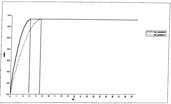
Figure 3.1 shows the shape of the value function under both scenarios. The functional forms assumed for the production and the utility functions in the

Figure 3.1: Value Function under Quadratic Utility: Deterministic Model

model, support a value function, which is strictly increasing until the critical point of capital stock, and then taking a constant value. This form of the value function is different than the form under the neo-classical scenario where the value function is strictly increasing in the whole domain. The critical point after which the value function becomes linear, is exactly the point where the bliss point of consumption becomes supportable in the infinite horizon. Below this level, thç value function displays a strictly increasing form as in the case of the neo-classical

model.

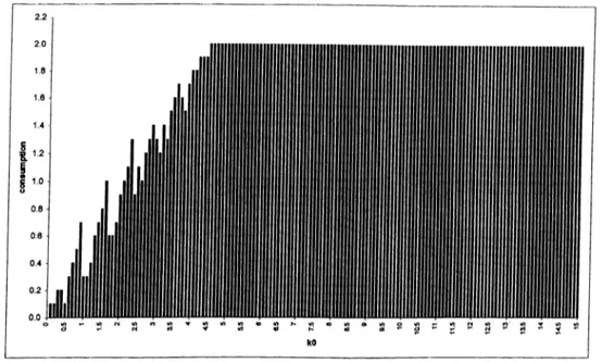
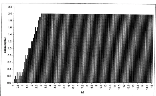
Figure 3.2 illustrates the shape of the consumption function vs. the initial value of the capital stock, for the first model {A' = 1.428). The figure illustrates that consuming at bliss becomes the optimal policy for capital levels that ai’e greater than which is computed to be 4.68 for the case under under consideration. The consumption function for the second model {A" = 1.68) is the same as the illustration in Figure 3.2, except that the critical is now 2.94; is given in Figure A .l in Appendix A.

Figure 3.2: Policy Function under Quadratic Utility: Expected Shock

Lastly I plot the number of divergent series vs. the initial capital stock, starting from the initial stock at f = 0 and moving the economy until the period t = 100. The exercise has been carried out 1000 times for each initial value of the capital stock and the number of strictly growing series of capital has been illustrated. Figure 3.3 shows the case for the first model with A' = 1.428. (The analogous Figure A .2 for the second model with A " = 1.68 is given in Appendix A.) The initial values of capital stock that are greater than kc, always supports

the economy on a path of sustained growth, as has been shown in Proposition 1. On the other hand, for any ko < kc, we observe no diverging series. Rather, a number of convergence points have been detected for the economies starting from any initial capital stock in this range. The observation of more than one convergence points however, is due to discretization of the state space into 0.1 grids, which has affected the dynamics of the algorithm.

Figure 3.3: Number of Diverging Series (out of 1000): A' = 1.428

3.5

Stochastic Case

This section presents the results of the simulation exercises adopted to the stochastic model. The results obtained in this section, generalize the results of the deterministic case to the stochastic environment. The technology faces productivity shocks, which has the ability to move the economy from one state to another. The social planner observes the value of the current-shock, but not the future values. Therefore the expected value of the consumption sequences to the planner are computed.

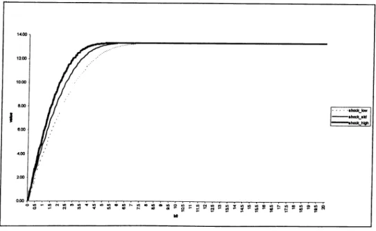
The illustration of the value function vs. the initial capital stock for each state of the random variable 2: is given in Figure 3.4. Here, we observe that the

Figure 3.4: Value Function under Quadratic Utility

value function takes the same shape as in the deterministic case but the point it becomes constant shifts to the right, as the initial shock reduces the productivity of the economy. The observation that after some initial level of capital, all three plots take exactly the same shape is also noteworthy. This shows the existence of an initial value of capital for which the planner takes exactly the same action no matter what type of shock is faced. The associated policy function figures revecil exactly the same scenario as Figure 3.2 and are given in Figures A.3, A.4, and A .5 in Appendix A.

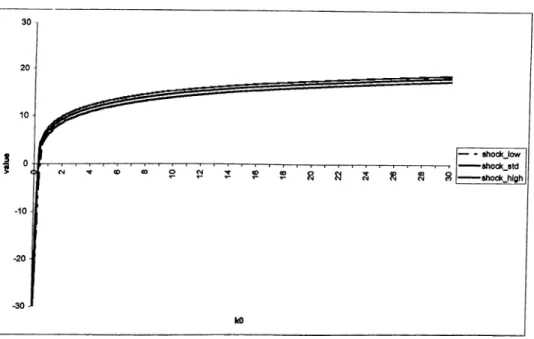
At this point, it would be interesting to observe the behavior of the value function under the same functional form for production, but the quadratic form of the utility changing to a strictly increasing, concave form from the form representing the bliss. For this observation, logarithmic preferences is adopted as the specialization of the utility function. U{0) is taken as —10 and a +3 is

added for all c > 0 for computational purposes. Figure 3.5 shows the behavior of the value function under logarithmic utility. The value function is observed to be strictly increasing as opposed to the case under quadratic form of the utility function. The policy function figures provide additional insight in making a comparison between the behavior of the economy under quadratic utility and the behavior under logarithmic utility. (Figures A.6, A .7, and A.8 in Appendix A, illustrate the policy functions for each state of the random variable, under logarithmic form.)

Figure 3.5: Value Function under Logarithmic Utility

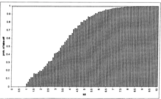
Considering the paths followed by the economy, the critical value of the capital stock, kc of the deterministic case now leaves its place to a probability distribution, over the initial values of the capital stock, ko denoting the probability of having a divergent sequence from each starting point. Figure 3.6 is obtained by a Monte-Carlo simulation exercise where the economy, starting from each initial value of capital is run for 100 successive time periods, each experiment being repeated 5000 times. The number of divergent series, for each starting point, divided by 5000, gives the approximate probability of take-off.

Figure 3.6: Probability of Take-off for Capital Stock

Divergence criterion taken while preparing the illustration in Figure 3.6 is that the capital stock at the end of period 100, reaches a sufficiently high value compared to the starting point. For a range of starting values ko 6 {0,0.1,0.2, ...9.9,10} the divergence criterion is the last period’s capital stock being greater than ¿loo = 10000. It is interesting that we have observed divergence with probability exactly equal to one for sufficiently high values of the initial capital stock. This shows the existence of initial values of capital stock that always take the economy into a sustained path of growth. On the other hand, for sufficiently low values of the capital stock, the probability for the economy to experience strictly growing sequences of capital approaches to zero. The equilibrium dynamics for these cases are well likely to drive the economy into a poverty trap.

The non-divergent sequences for a large range of the initial capital stocks, follow a very similar pattern as the deterministic case and show different loutes of convergence. The steady-state behavior under stochastic case of couise, is

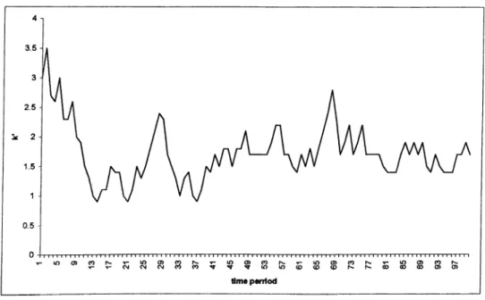
expected to be identified by a distribution over a certain range of capital stocks. As an illustration of convergence and divergence paths, Figure 3.7, Figure 3.8 and Figure 3.9 show how the economy moves starting from t = 0 with an initial capital stock, ko = 3.9 until t = 100. Figure 3.7 here can be identified as the illustration

Figure 3.7: Sample Path of Convergence: ko = 3.9

of an economy which is pushed into low levels of capital stock by unfavorable shocks to productivity, and seems to be “trapped” in this situation. Figure 3.8 shows an economy which, after 100 time periods, still have not achieved a way to sustained growth, but living in cycles of booms and busts. In Figure 3.9 we observe an economy, which has the same starting point as the economies of Figures 3.7 and 3.8 but has achieved its take-off into sustained growth.

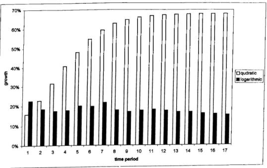
Once we have observed the existence of divergent paths, it is also possible to give a comparison of growth rates under the model adopting quadratic form of utility, and the model adopting logarithmic utility. As an illustration, an economy starting from an initial level of capital stock, ko = 3.4 is taken. The deterministic model with A" = 1.68, adopting quadratic utility and a deterministic model with

Figure 3.8: Sample Path of Convergence: ko = 3.9

a logarithmic utility function are used to compute the growth rates. Figure 3.10 shows the growth rates in each period under both models. The growth rate under the classical endogenous growth model is more or less constant, as pointed out by the current endogenous growth theory, whereas the growth rate under the model with quadratic utility is increasing in each period.

Figure 3.9: Sample Path of Take-off: ко = 3.9 70% 60% 50% 40% □q u d ra tic logarithmic |

Figure 3.10: Comparison of Growth Rates for Divergent Seiies. 3.4

Chapter 4

Conclusion

This study has constructed a one-sector, discrete time stochastic model of optimal growth, where households have a point of maximum attainable utility in their consumption sets. The behavioral assumption that households have a bliss point, has substantially changed the results of the current endogenous growth theory.

The equilibrium of the Ak-iy^e. of endogenous growth model, identified by sustained growth of per capita income, leaves its position to the existence of multiple steady-state equilibria, if a quadratic utility function -representative of households having bliss- is assumed instead of a strictly increasing one. There are equilibrium paths, illustrative of the hypothesis of the neoclassical theory, which converge to a steady-state. There are also equilibrium divergent paths which exhibit endogenous growth theory. An economy can move to one equilibrium or the other, depending on the initial state. Specifically, this thesis provides a simple analytical interpretation of the empirical evidence on the existence of both paths of poverty and paths of perpetual growth.

Deterministic model of Section 3.3 shows the existence of a critical level of initial capital stock, above which sustained per capita growth is achieved. The mechanism behind the observation of sustained growth for a model economy is as follows: For initial capital values which are greater than some critical value, the constant returns to scale technology provides the economy with an output level

where it becomes possible to consume at bliss level in the current period, and to consume always at that level thereafter. The economy follows a path where capital stock is strictly increasing, reaching to infinity in the limit. For low levels of initial capital stock however, the equilibrium is identified by convergence to a steady-state, which can be interpreted as a stationary trap at some level above the state of zero-income.

Introduction of a random element in the production function, changes the results in a way to “soften” the sharp threshold observed in the deterministic case. A sequence of favorable shocks may well function as sharp stimulus in some form of technological innovation, or education, causing the “big-push” . The economy then, experiences a path of sustained growth. On the other hand, an economy, facing a sequence of unfavorable shocks, may find itself locked in an underdevelopment trap. Figure 3.6, showing the probability of take-olf from each initial state portrays that the model constructed in this study, accounts for the possibility of both scenarios to take place.

Besides the identification of poverty traps and paths of permanent growth, this study also captures the situation that, countries which are identical initially, may be driven by different conditions to alternative destinies of making the “miracle” and trapping in stagnation. Figures 3.7, 3.8 and 3.9 depict these scenarios which are not far away from what we observe in actual world.

Approaching the problem of combining the hypotheses of neoclassical theory with the endogenous growth theory by making the behavioral assumption of a bliss point in households’ consumption sets, this study differs from the other studies of the literature. The models of Dechert and Nishumura and Zilibotti which are also constructed in an environment of infinitely-lived households, bear on the changes in the form of the production function, depending on the level of the capital stock of the economy. The simple model constructed in this thesis, point to the importance of the assumption on the household utility functions; a

fact that may well change the policy implications at times.