Analysis of assembly systems for interdeparture time
variability and throughput
IHSAN SABUNCUOGLUI, ERDAL EREL" and A. GURHAN KOK3
IDepartment of Industrial Engineering, and 2Faculty of Business Administration, Bilkcnt University, Ankara, Turkey 06533
E-mail: [email protected]
30perations and Information Management Department, University
(If
Pennsylvania, Pili/adelphia PA 19104, USAReceived January 1999 and accepted April 2001
This paper studies the effect of the number of component stations (parallelism), work transfer, processing time distributions, buffers and buffer allocation schemes on throughput and interdeparture time variability of assembly systems, As an alternative to work transfer, variability transfer is introduced and its effectiveness is assessed. Previous research has indicated that the optimal throughput displays an anomaly at certain processing time distributions and, this phenomenon is now thoroughly analyzed and the underlying details are uncovered. This study also yields several new findings that convey important practical implications.
I. Introduction
In this paper, we consider the problem of designing an assembly system in which parts produced at two or more component stations are fed into an assembly station. In general, assembly systems are built from three main building blocks: (i) serial; (ii) merging; and (iii) splitting (or competing) configurations. Most of the existing work to date has been conducted on serial systems even though the merging and splitting configurations are commonly encountered in practice. In our study, however, we con-centrate on the merging configuration and examine its various design characteristics.
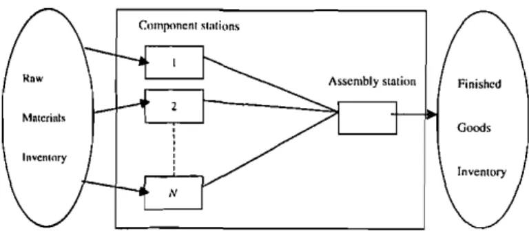
The system under consideration is an assembly system containing two or more component stations and an as-sembly station with unlimited raw materials and finished goods inventory capacities. In the unbuffered system, there is no storage space between the component stations and assembly stations (Fig. I). On the other hand, in a buffered system, there is storage space downstream of the component stations in which WIP inventory can be temporarily stored. In the unbuffered case, the assembly station does not start processing unless all items are transferred to the assembly station from the component stations (i.e., the assembly station does not start pro-cessing until a part from each feeder station becomes available). If a component station completes work early, it is blocked. On the other hand, the assembly station starves if one or more items are not ready from the component stations. Consequently, buffers reduce the incidence of blockage and starvation. Even though 0740-817X ©2002 "II E"
the main emphasis of this paper is on an unbuffered configuration, we test the sensitivity of the results to the buffered case. Since the receiving area upstream of the component stations has an unlimited supply of raw ma-terials and the shipping area downstream of the assembly station has an unlimited finished goods buffer capacity, the component stations never starve and the assembly station never becomes blocked. In common with the previous studies reported in the literature, all component stations are assumed to be identical and independent of each other.
In this study, we consider a system in which all the stations are perfectly reliable and have a 100% yield rate (i.e., no breakdowns, scraps, waste and absentee-ism). We also assume that the system operates under a push mode. In other words, the component stations continuously process raw materials as long as they are not blocked and the assembly station operates as long as it is not starved. In contrast, demand triggers the production process in systems operating under the pull mode.
The system described above can be viewed as a simple system. However a thorough analysis of such a system can provide important insights into the better under-standing of more complex real life systems. Also, this simple merging configuration constitutes a major building block of assembly systems encountered in practice. As previously noted by Powell and Pyke (1998), these sys-tems are also common in several mixed model automated processing and manually operated assembly systems (e.g., ready-to-wear apparel production).
Fig. I. Schematic viewof an assembly system,
A key criterion in the design and operation of assembly systems has been the throughput which is measured as the number of units produced per unit time. Output vari-ability (or interdeparture time varivari-ability) is also impor-tant especially in today's highly dynamic and stochastic environments, since a highly variable input or output process makes planning difficult and causes the per-formancc to deteriorate significantly. For example, Hendricks (1992) and Hendricks and McClain (1993) study the output processes of serial production lines by observing the first and second moments of the interde-parture time distribution. Hence, practitioners designing such assembly systems should consider interdeparture time variability in addition to throughput. Here, inter-departure time variability is defined as the standard de-viation of the time between consecutive departures of finished prod ucts from the system.
In this study, we consider both throughput and inter-departure time variability and analyze the effects of de-sign factors such as parallelism (given by the number of component stations), processing time distributions, work and variability transfers from the assembly station to component stations, buffers and buffer allocation schemes. We also study the so called "intrinsic behavior of the optimal throughput for some processing time dis-tributions" (Baker et al., 1993; Rekhi et al., 1995) and uncover the underlying details.
The rest of the paper is organized as follows. In Section
2,
we summarize the relevant literature on assembly sys-tem design. In Section 3, we present the proposed ap-proach, system considerations, and experimental design. The results of simulation experiments are presented in Section 4. In Section 5, we explain the intrinsic behavior. Later, we extend our analysis to the buffered case in Section 6. The paper ends with concluding remarks and suggestions for further research in Section 7.2. Literature survey
There arc only a few limited studies on this problem. They arc briefly summarized in chronological order below.
Baker et al. (1990) examine the design of balanced as-sembly systems with variable processing times under two
Sabuncuoglu et al.
loading mechanisms. The term "balanced" refers to identically distributed component and assembly station processing times. For all processing time distributions, the authors observe that the push mode results in a higher throughput than the pull mode since an assembly system utilizes the virtual buffer that exists in the assembly sta-tion under the push mode. The authors also analyze the effects of buffers on the throughput of assembly systems containing 'two feeder lines where each feeder is a serial line. They note that the results from the serial line re-search generally apply to such systems. In addition, the authors observe that a small buffer is sufficient to recover the significant portion of the lost capacity and that equal buffer allocation is desirable for these systems.
Later, Baker et al. (1993) examined the problem of allocating a fixed amount of work to stations in an as-sembly system operating under the push mode. For sys-tems of up to four component stations with exponentially distributed processing times, Markov analysis was used, whereas simulation was used for other distributions and larger systems. Their basic finding is that the throughput can be improved by transferring work from the assembly station to component stations. The authors also study two specific unbuffered assembly systems for exponential and uniform processing time distributions. The first one is a system with two feeder lines where each feeder line is composed of two stations. Their results indicate that throughput is maximized by allocating more work to the initial stations and less work to the final stations of the feeder lines and assembly station. The second system in-volves two or more component stations in parallel. The results show that optimal throughput is a decreasing function of the number of the component stations. However, this phenomenon is not observed for the uni-form distribution; instead, optimal throughput displays a small peak in a specific range. We call this anomaly "hump behavior" in this paper. In a later study (but published earlier), Baker (1992) presents a brief survey on serial lines and assembly systems. He notes that the above unexpected behavior might be due to the lower coefficient of variation (CV) of the uniform distribution.
Bhatnagar and Chandra (1994) examine the impact of different types of variability (processing time, unreliable stations and imperfect yield) on the throughput of as-sembly and competing systems. They find out that theCV
of the processing times is a critical criterion for studying the impact of processing time 'variability in assembly systems.
Rekhi et al.(1995) studied assembly systems with up to 100 component stations for exponential, uniform, gamma and normal processing time distributions with different CV's. The results indicate that as the number of com-ponent stations increases, the optimal throughput steadily deteriorates for the distributions that have small tails such as exponential and high-CV gamma distribu-tions. However, they observe a hump behavior for those
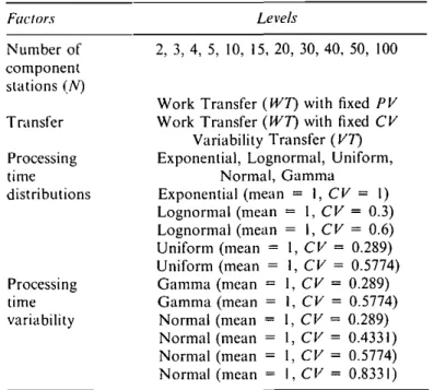
Table J. Experimental factors and levels
In a merging configuration with an equal amount of work at each station, the assembly station acts as a bot-tleneck since it is dependent on component stations. In such a system, favoring the bottleneck station in order to improve the system performance can be achieved either by transferring the work and/or variability of the bot-tleneck station (assembly station) to other non-botbot-tleneck stations (component stations) or imposing planned overtime work on the assembly station. Here, work transfer (WI) refers to shifting some work from the as-sembly station to the component stations by keeping the total work content of the system constant. Specifically, some portion of the mean processing time of the assembly station is transferred to the component stations. For ex-ample, consider a two-component station (i.e., one as-sembly station and two feeders) system with one unit of mean processing time and one unit of variance on each station. As depicted in Fig. 2a, the assembly station acts as a bottleneck in the system. One possibility to relieve the bottleneck station is to transfer some work, say 0.2 units of work, from the assembly to the component sta-tions that results in 1.1, 1.1, and 0.8 units of work (mean processing time) in the component stations and assembly station, respectively.
Note that the work transfer can be achieved by either keeping the coefficient of variation (CV) or processing time variability (PV) constant (Fig. 2). In practice, the CV-fixed case arises when the variability is mainly caused by internal factors such as, worker qualification, part and process characteristics, whereas the variability in the
PV-fixed case is mainly caused by external factors such as the nature of work environment, level of automation, etc.
distributions that have long tails such as normal or
low-CVgamma distributions. The authors explain the hump behavior as being a result of the long tails of the above distributions. In this study, we further examine this be-havior and uncover the underlying details.
In another study, Baker and Powell (1995) present a predictive model for the throughput of an assembly sys-tem with two component stations. They develop a dis-tribution-free method to evaluate alternative system designs and claim that the algorithm performs well in terms of the accuracy of the predictions. Simon and Hopp (1995) analyze an assembly system with two component stations. There are finite buffers between each component and the assembly station. The authors develop a sto-chastic model to estimate the steady-state average throughput and inventory level performances.
Finally, Powell and Pyke (1998) analyze optimal buffer allocations for unbalanced assembly systems with two or three component stations. The authors suggest methods to find the optimal location for the first buffer. The results indicate that the optimal buffer location depends not only on the mean processing times, but also on the variability of the processing times.
3. Proposed study
As can be noted from the literature review, there are only a few studies that analyze the merging assembly config-uration. Furthermore, the problem is only studied for the throughput measure by considering some design factors. For this reason, there is a need for a thorough analysis that address the following research issues:
I. An analysis of the interactions between various factors such as the number of component stations, processing time variability, work or variability transfer between stations for throughput.
2. An explanation of the hump behavior.
3. Repeating the analysis in I and 2 for interdeparture time variability.
4. Testing the sensitivity of the result to the buffered case.
.We analyze these research issues in the following sections. 3.1. Experimental settings
We use four experimental factors with their levels given in Table I: system size, transfer type, processing time dis-tribution, and variability. System size, which determines the complexity of the system, is defined by the number of component stations. The previous studies on assembly systems indicate that the system performance is strongly affected by the system size. As seen in Table I, we have II levels of N, ranging from the most basic system (N
=
2) to a very large system (N=
100).Factors Number of component stations (N) Transfer Processing time distributions Processing time variability Levels 2, 3, 4, 5, 10, 15, 20, 30, 40, 50, 100
Work Transfer (WI) with fixed PV
Work Transfer (WI) with fixed CV
Variability Transfer (VI)
Exponential, Lognormal, Uniform, Normal, Gamma Exponential (mean
=
I,CV=
I) Lognormal (mean=
I,CV=
0.3) Lognormal (mean=
I,CV=
0.6) Uniform (mean=
I,CV=
0.289) Uniform (mean=
I,CV=
0.5774) Gamma (mean=
I,CV=
0.289) Gamma (mean=
I,CV=
0.5774) Normal (mean=
I,CV=
0.289) Normal (mean=
I, CV=
0.4331) Normal (mean=
I, CV=
0.5774) Normal (mean=
I,CV=
0.8331)(II) (b) 0.85 - , - - - , 0.65
.\
o.ao \.
,\
-,.,
<,
.~.---.---.
:; 0.750-f
~ 0.70Fig. 2. Thework transfer alternatives: (a) WTwith a fixedCV; and (b) WTwith a fixed PI/.
Number of component stations(N)
3.2. Simulation model 60 70 80 90 100 50 30 40 10 20 0.80+ - - + - - + - - + - - + - - + - - + - - + - - + - - J - - - 1 o
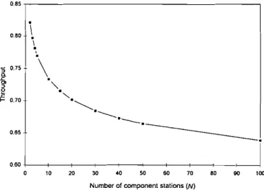
Fig. 3. The effect of parallelism (N) on throughput in the bal-anced case for lognormal times with CV
=
0.289.experiments because of its flexibility and positive skew-ness. It is also one of the most suggested distributions in the literature. The exponential distribution is used to see the effect of a high variance case. The other distributions (gamma, normal, and uniform) are employed to investi-gate the hump behavior. Note that we use the same dis-tribution function for both the assembly and component stations. In the simulation experiments, processing times are generated independently for each component station from the same distribution function (i.e., random variates are generated at each component station whenever needed). At the assembly station, we use the same type of distribution function with different parameters due to work and variability transfer.
The simulation model is developed using SIMAN. The Welch approach (Law and Kelton, 1991) is used to de-termine the warm-up period (300 observations). Relevant statistics are collected in steady-state conditions using the replication/deletion method. Specifically, 20 replications each with a length of 2000 observations are taken with an initial condition of an empty state (i.e., the data analysis is performed for 40 000 observations in steady-state conditions). A total of 20 simulation replications are taken to achieve a satisfactory level (at most 1%) of the relative accuracy (half width of the confidence interval divided by the estimate of the quantity of interest). Spe-cifically, we used the confidence interval approach for the paired-t test to assess the significance of the differences between results obtained at various experimental points. In our study, IDTVis measured by using the average of the sample standard deviations of 20 replications. Even though this is not an unbiased estimator of the popula-An alternative way of relieving the bottleneck station is
to transfer some portion of variability of the assembly station to component stations. This is called variability transfer (VT) and it shifts the variance of the assembly station to the component stations by keeping the sum of the variance of the processing times constant. In practice, the variability transfer can be achieved by allocating more experienced/trained workers to the assembly station.
We usc the following three-clement notation (i/ii/iii) to describe the main characteristics of the experimental setting.
i. Type of transfer: Work transfer(W7) or variability transfer (V7).
ii. Coefficient of variation (CI/) or processing time variability(PI/) is kept constant during the transfer. iii. Objective function: maximize throughput (7) or
minimize interdeparture time variability (IDTI/). The factors in the first two entries have been discussed previously. Note that the second entry is left blank for variability transfer since neither CV nor PV is kept con-stant. The third entry in this notation is reserved for the performance measures (Tand IDTI/). If this entry is left blank, it indicates that an optimization is conducted for either Tor IDTV by generating the entire search space (i.e., complete enumeration) and selecting the best per-former. For example, the notation WT/CV/- of Sections 4.1.1 to 4.1.4 represents the case in which an optimal Tis investigated as work is transferred from the assembly station to the component stations. Here, the optimal
Tis
obtained by searching all possible ways of work transfer that yield the maximum T for a given number of com-ponent stations (N). As a result, Fig. l4a.b (optimal T versus N) is obtained by plotting the best T values ex-tracted from Fig. 4a-c (T versus W7).
In this study, we consider five different distribution functions for the processing times. A list of these distri-butions and their variability levels arc given in Table I. These distribution functions and their parameters are selected from the literature based on previous theoretical and empirical studies (Knoll and Sury, 1987; Bakeret al., 1990). We mostly used the lognormal distribution in our
__._Na 10 - + - N a S (a)
:::L...
I I ......
0.55: •••· .. ···... • •••••i
0.50L :-~
045V
040L
"
0.35 0.30 ~---;--+---+-~---+--'==;::::::::'J 1 1.05 1.1 1.15 1.2 1.25 1.3 1.35 14 1.45 1.5Moan processing time of component stations In this section, we present the results of our simulation
experiments. First, we examine the effects of the experi-mental factors (i.e., parallelism, work transfer, variability of processing times) on throughput. This is followed by the analysis for the interdeparture time variability
(IDTV). We then compare work and variability transfers in terms of throughput and IDTV. We should also point out here that the results presented below are tested for statistical significance at C(
=
0.05.tion standard deviation, it is a practical measure and produces a reliable estimate for the variability.
4. Computational results (b)
..
" . • NaZ - a - N _ 3 _ _ N_5 _ _ N_10 - . - N - l 0 1.05 1.1 1.15 1.2 1.25 1.3 1.35 1.4 145 1.5Mean processing time of component stations
0.80 070
.1···· ·..····..·
.
.." ".. .. ... .. ...
.
0.65~::---
'. '" ••••••••••••••• 0 6 0 r/ ••••• 0.55L---;----+--+---;--- --I 1 1.05 1.1 1.15 1.2 1.25 1.3 1.35 14 145 1.5Mean processing time of component stations
0.65 0.55+----.----+---;-_--+---;--1 0.60 :::: l v · ·::: ...
?':::;'"
•. & " . . . . : : • •...
,-.
:; 075 ":::" ~ ..
.•.
:.:.:.:
...
o •.••• .i:: 0.70 " . f- • " . (e) 0 . 8 5 , - - - r - - : : - 7 . " : : : - h :; 0.75 0. s: OJ :Je
s:f-Note also that the maxima of these curves correspond to optimal Tvalues associated with N.
The practical implication of the above result is that a certain amount of work transfer from the assembly to the component stations helps to raise the throughput level without employing any additional resources (e.g., buffers). Fig. 4. The effect of WTjCV(- on throughput for: (a) expo-nential processing times; (b) lognormal processing times with CV
=
0.3; and (c) lognormal processing times with CV=
0.6.4.1.2. Effect of WT/C
V(-When a certain amount" of work is transferred from the assembly to the component stations by keeping CV con-stant (i.e., the variability of the processing times is pro-portional to the mean), Tincreases up to a level and then decreases, resembling a concave function (Fig. 4(a-e». Note that the decreasing behavior is not observed for large Nsince the amount of work in the assembly station is not sufficient to raise the mean processing time of the com-ponent stations. Prior to work transfer, the assembly sta-tion acts as the bottleneck stasta-tion. Hence, work transfer favors the bottleneck station and leads to an improvement in T.However, after a certain amount of work transfer, the component stations become a bottleneck and conse-quently any further work transfer leads to a decrease in T. 4. I. I. Effect of parallelism (N)
Throughput of a balanced system (with the mean pro-cessing times set to one) decreases at a decreasing rate (Fig. 3) as N increases. This is due to the fact that, as parallelism increases, coupling in the system increases, synchronization of the components becomes more diffi-cult and thus T decreases. This result is previously re-ported in the literature (Bakeret al., 1993). Note that the rate of decrease slows down as N increases, since the ef-fect of adding one more station to a larger system (e.g., N
=
50) is less significant than a smaller system (e.g., N = 2).The above result has important practical implications since the decreasing behavior of T reinforces the design for assembly principle: designing products with the
min-imum number of component parts.
The results on throughput (n are itemized below. A few of these results are confirmations of previous findings; we present them in order to give a complete picture and validate our model.
4.1.3. Interaction effect of' WT/CV/- and parallelism Theeffectof work transfer on Tis pronounced for large N, since there is more improvement potential in such systems (sec Fig. 4(a-e». This means that the capacity lost due to coupling in the system can be regained by work transfer to a greater extent in large systems than in small systems.
4.1.4. Interaction effect of' WT/CV/- and CV
As depicted in Fig. 4(b and c), the rate of improvement in T is smaller in the high CV case (e.g., for N = 10, the improvement after 0.02 units of work transfer is 5.11 % for a low CV while it is 4.44% in the high CV case). This is been usc, in the high C V case, the positive effect of work transfer becomes smaller due to increased in the system. In other words, to obtain the same percentage of im-provement, one needs to make more work transfer in the high CV case than the low CV case. When the simulation experiments arc repeated at very high CV (e.g., CV= 1.5), we observed the same behavior.
4.1.5. E/j'eel.\· of WTj P V/- and interactions with parallelism and P V
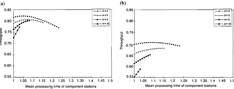
As discussed earlier in the paper, the second type of work transfer is accomplished by keeping PV constant. This means practically that more experienced workers and/or faster machines arc shifted to the component stations. When this situation is analyzed, we observed the same concave behavior of Twhich has been already elaborated in Section 4.1.2.
Note that this concave behavior can only be shown for some ranges of the mean processing time of lognormal distribution (Fig. 5(a and bj), This was mainly due to the
difficulties encountered in generating lognormal random variates for small mean values and very large variances.
4.1.6. Effect of
VTj-/-As variability is transferred from the assembly station to the component stations (i.e., the standard deviations of the processing times of the component stations increase), Tincreases (Fig. 6 (a and b». However, the change in Tis relatively less significant in this case than the PVOl'
C
V-constant work transfer cases. This result is analogous to the previous findings on serial production systems: the effect of processing time variability on Tis much less than the mean of processing time (Lau, 1992; Erel et al., 1997). Again, the same behavior is observed in the very high CV case.4.1. 7.Interactions ofVTj-/- withparallelism andPV When Fig. 6(a and b) is carefully analyzed, we observe a tendency that the increase in T is greater in large systems (i.e., more component stations), even though the im-provement is not statistically significant. As discussed in Section 4.1.3. this result is due to the existence of more improvement potential in such systems.
4.2. Results011interdeparture time variability
We present the results on IDTV in the same order as throughput.
4.2.1. Effeel ofparallelism (N)
As N increases, IDTV increases at a decreasing rate (Fig. 7) due to more coupling in such systems. Similar to T, the effect is less significant in the high parallelism case. This suggests that systems with fewer component stations
• N-2 - ..-N-3 ---+--N-S ______ Nil 10 0.80 0 . 8 5 , - - - c : : = ; ; ; - n (b)
I
0751
e
0.70 •• _.r=
I....
.
A " ,.£ .. 0 . 6 5 · V 0.60 0.551
1 1.05 1.1 1.15 1.2 1.25 1.3 1.35 1.4 1.45 1.5 Mean processing time of component stations- . - N - 2 - . - N : 0 3 ---+--N- 5 _ _ _ N-10
...
..
1.05 1.1 1.15 1.2 1.25 1.3 1.35 1.4 1.45 1.5 Mean processing time of component stations0.55 +--+---'--+--+--+----+--...,---+--+---J 1 (1I) 0.85, - - - 1 - - - - : : - - - - ; : : : 7 1 - 1 0.60 0.65
s
,g.
0.75 Cl ::>e
r=
0.700.60 __._N-S _ _ Na1Q - A - N - 3 -a-N-2 (b) 0.85
1
0001
I :::
0 _ 0 _ 0 _ _ 0 _ 0 _ 0 _ 0 _ 0 _ 0 _ 0 _ 0 _ 0 _ 0 - 0e
I ~-.-.-.
0.65c '. ' - - 0 ' - ' - ' - '-
...
0.60 0.55---+---+---=+==::::::..j
0.6 0.6::: 0.64 0.66 0.68 0.7 0.72 0.74 Std.dev. of processing time of component stations 0.31 0.32 0.33 0.34 0.35 0.36Std.dev. of processing time of component stations
0 0 0 0 0 - - - 0 0 ~
.
.
.
.
.
~ ~ - __ N=2 -A-N=3 ~N=5 _ _ N=10 0.55 0.3 0.65 0.80 :; 0.75 0-J:: 0> :J 0.70e
J:: f--(a) 0.851
Fig. 6. The effect of VT/-!- on throughput for lognormal processing times when: (a)PV
=
0.3; and (b)PV=
0.6.0.50 0.40 ~0.45
9
0 . 5 5 , - - - 1----0
--0
--0
..-/0
. / a /-I
° o,
° I ° 0.35I----+--+--+----;---+--+--+----;~--+--<o
10 20 30 40 50 60 70 80 90 100Number of component stations(M
Fig. 7. The effect of parallelism (N) on interdeparture time variability in the balanced case for lognormal processing times withCV= 0.289.
are more advantageous for JDTV from the system de-signer perspective.
4.2.2. Effect of
WT/CV/-We identified two cases each of which is explained below. The first represents the simple situation whereas the sec-ond is a relatively complicated case that requires further analysis.
4.2.2.1. Exponential distribution case. Similar to the throughput case (Section 4.1.2), the performance of the system improves by work transfer up to a certain level and then starts to deteriorate (Fig. 8a). However
differently to the previous case, the, JDTV behavior is a convex function of the work transfer. Similar obser-vations are made in the hyper-exponential case.
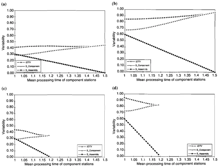
4.2.2.2. Lognormal and uniform distributions cases.
Un-like the exponential case, the behavior of the JDTV as a function of work transfer is a complex function. In this case, as seen in Fig. 8(b-t), the function is not unimodal with no apparent explanation. Hence, we perform ad-ditional experiments to understand this interesting be-havior. Specifically, we measure the JDTVin terms of its components: the variability of interarrival times to the assembly station (called the S_Component) and the variability of the assembly station (called the S_Assem-bly). Figure 9(a--<l) illustrates the behavior or these two components. Since CV is kept constant during the work transfer, S_Assembly decreases linearly with work transfer where the slope is higher in the high parallelism and high CV cases. On the contrary, the S_Component increases with work transfer because the P V of com-ponent stations increases. As a result of the combined effect of these two components, JDTV decreases as a function of work transfer in the high parallelism and high CV cases, but it increases in the low parallelism and low CV cases, Figure 8(e and f) also supports the above observations for uniform distribution. We also note that the results of a lognormal distribution with CV=
I (Fig. 8d) are very similar to the exponential distribution case (Fig. 8a). This implies that the behav-ior of the JDTVapproaches the convex behavior of the simple case.The above discussion suggests to practitioners that one should be cautious when implementing work transfer in the low CV and low parallelism cases since the complicated behavior of JDTV can conflict with T.
(a) 2 . 0 0 , - - - , (b) 0 . 5 0 , - - - , 1.90 1.80 ~1.70
9
1.60... ··-.-"'.3
j...
.:~.:.:...--"'-5
•• • .... • •••'orlm.=.:!!:':'.:.'"t-"-->--+--';==.==N::'::lO::j
1.40~~···"-~---1.05 1.1 1.15 1.2 1.25 1.3 1.35 1.4 1.45 1.5 Mean processing time of component stations0.48 046 0.44 l \ •••••• ~~
...••....
.
...
~ ~.;~r::~\.t~
:
::::::::: .
0.36 ,....---,-, _._N_2 0.34-._N·'
0.32 ---+-N-5 0.30L--~~ ---<-~---.;=::::;:::::::J 1 1.05 1.1 1.15 1.2 1.25 1.3 1.35 1.4 1.45 1.5 Mean processing time of component stations (c) 1 . 1 0 , - - - ' - - - , 1.05 1.00 -a-N=2 _ _ NaS - " - H - 3..'
..
,...
.'
...
.."
1.60 ..~
. . . . .. . .. .. .. .. .. . . ..
.
....
1.50 •••••••••...•...
1.90 ----N-l0 1.80 (d) 2 . 0 0 , - - - , - 0 - N · 3 ---+-"'-$
___+__H_l0 0.75 0.95.
•• - • ' ~...
~0.90... • ••••••• :.:.:: ••••• I 1\" ·t· "'!e ;.~.: . 0.85···'\:· .~ 0.80Mean processing time of component stations
...
.
..
.. .. ---+--"'=5 ---+--N-l0..
'..,
.'...
.
...•...
"£. • •••••••••••••• 0.45 0.50 (f) 080~ 0.75 ' .• 0.70 0.65 0.60 ~ 90.55 ---+--"'·'0
_ _ "'''5 - ..- H - 3...
(c) 0.45 [0.43 I 0.41039 • ••••••"'1
.:"
:.:.:...
.
...
0.37 •.•.•.•.•.• '. ~0.35 9 0.33 0.31 0.29 0.27 0.251--~-~~-~~--+--~---I--..-...lj 1 1.05 1.1 1.15 1.2 1.25 1.3 1.35 1.4 1.45 1.5Mean processing time of component stations Mean processing time of component stations
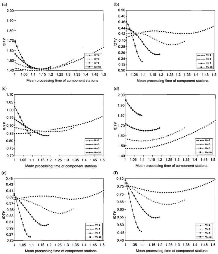
Fig.II. The effector WTjCV/- on interdeparture time variability for: (a) exponential processing times; (b) lognormal processing times with CV
=
0.3; (c) lognormal processing times with CV=
0.6; (d) lognormal processing times with CV=
1.0; (e) uniform processing limes with CV=
0.289; and (f) uniform processing times with CV=
0.5774.4.2.3. Effect of
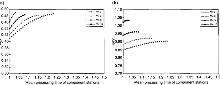
WTjPV!-As seen in Fig 10(a and b), IDTVfirst increases and then stabilizes at some level as work is transferred from the
assembly station to the component stations. This is probably due to the increase in mean processing times of the component stations. Note that the curves could not be
(a) 1 . 0 0 , - - - , 0.90 O.BO 0.70 (b) 1.00~ , " .. 0.90
...
•••••••••.:."' ......
o
BOt-··· ···
..
• ..10 .10 .10 .. 0.70...
..•.•., .. 1.05 1.1 1.15 1.2 1.25 1.3 1.35 1.4 1.45 1.5 Mean processing time ofcomponent stations-o-IOTV
j
- ..-S_Compcnent ---+--S_Assem,ty 0.30 0.20+, _ 0.10 O.OO+'==~~~~~--+-_I_-_--+-_I_-~~ 1 0.20+,---==::---"';-... 040 ••••••••••••••••••••••••••••••••••~~n••••~• • • • • • • • •. L-·
..
.10 .. 0.30 _ .' " ~ 0.60 ~ 0.50 'C ~ (c) 1 . 0 0 , - - - , 0.90 O.BO 0.70 (d) 1 . 0 0 , 1 - - - _ 0.90f
O
000
...
0.80 ...: :.:.::... . . . .10 0.70 ... -.-IDTV -.-IDTV -&-S_Component ---+--S_Auembly 1.05 1.i 1.15 1.2 1.25 1.3 1.35 1.4 1.45 1.5Mean processing time ofcomponent stations
£;'0.60 :00.50
'"
'C ~ 0.40 0.30 0.20 0.10 O.OO.\-~--+-.-~~-_I_-_----.b~~;;;;;;;;2=d...I 1 .~0.60 ~ 0.50~ ~.:~
[Oo
00::::::::::"..
0:20<,
0.10 .~
0.00.\---+-~-~~--+---.,----1=~=F:;:;;;~Lj 1 1.05 1.1 1.15 1.2 1.25 1.3 1.35 1.4 1.45 1.5Mean processing time ofcomponent stations
Fig. 9. The effect of WT/CV/- on interdeparture time variability and its components for lognormal processing times when: (a) N
=
2, CV=
0.3; (b) N=
2, CV=
0.6; (e) N=
5, CV=
0.3; and (d) N=
5, CV=
0.6.completed because of the difficulty encountered in gen-erating lognormal random variates for small mean values and very large variances.
4.2.4. Effect of
VTj-/-IDTV decreases as more variability is transferred to the component stations (Fig. II (a and b)). This is because the assembly station, that acts as the bottleneck station, is favored by variability transfer and consequently the I DTV decreases. In practice, this suggests that one should assign less variable operators, machines or other re-sources to the assembly station.
4.2.5. Interaction effect of VTj-/- and parallelism
As seen in Fig. II (a and b), the rate of improvement in IDTV, as variability is transferred from the assembly to the component stations, is more significant in the high parallelism case than in the low parallelism case due
to more variability transfer possibilities IJ1 large sys-tems.
4.2.6. Interaction effect of VT/-/- and PV
The percentage improvement in IDTV, as variability is transferred from assembly to component stations, is less in the high PV case (Fig. II(a and b)). As a result, the potential benefits of variability transfer are not realized to their full extent due to the highly variable environment.
As a closing remark in this section, we can con-clude that work and variability transfers are effective tools to improve system performance both in terms of T and IDTV, especially in the high parallelism and low CV cases.
4.3. Analysis ofthe correlation of the output proce.u
We also analyze the correlation structure of the output process. Specifically, we consider the effects of correlation
- ..- N .. 3 _ _ N=10 ____ HOllO _._Nra2 _ .._N_3 _ _ N-S ~ il.•••••• 00.90 ...,.•.•.<10... • •••••••••••• - I •••••••
~::~j
....
0.75. 0.70 ---+--+---+--+-~---+--+---+--+--1 1.05 1.1 1.15 1.2 1.25 1.3 1.35 1.4 1.45 1.5 Mean processing time of component stations(b) 1.10,---~--__n 1.05 -+--N"S - e - N .. 2 1.05 1.1 1.15 1.2 1.25 1.3 1.35 1.4 1.45 1.5 Mean processing time of component stations
...
...
...
..
....
..
.
.
,,;..
..
"..
0.42r:".··
~.
90.40 0.38 0.36 0.34 0.32 0.30.l--->---+--<---+---+----<-_i_-+---+---j 1Fig. 10. The effectof WTjPVj- on interdeparture time variability for lognormal processing times when: (a) PV= 0.3; and (b)
I'V=0.6. - . - N " , 2 -6-N=3 -+--N-S _____ N=10 0.95 ~0.90
-
0.85-'---
I '---.--A
.-.-:~,~ 0.80 ~'"",.--
<:--.--0.75 ..'-... ---. __ •--.
0.701----+---+----+---+---0---+---1 0.6 0.62 0.64 0.66 0.68 0.7 0.72 0.74Std.dev. of processing time of component stations (b) 1.10r---r-~~ 1.05 -+--N=S _______N '"10 _ . N:2 - ..-N_3 0.32 0.34 0.36 0.38 0.4 0.42 0.44 Std.dev. of processing time of component stations (a) 0.50r---,---::~ 0.48 0.46 0.44
~,
0.42t ~.
90.40 1 \ 0.38 :~ 0.36 '\."-., 0.34 '\."-.,. 0.32 • "'. 0.30+--_--O---O---f---+----+-~ 0.3Fig. II. The effect of VTj-j- on interdeparture time variability for lognormal processing times when: (a) PV
=
0.3; and (b)I'V= 0.6.
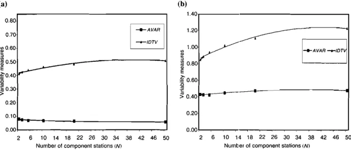
on IDTV for system size (N), work transfer (W7) and variability transfer (V7). The objectives of these experi-mentations are: (i) to see if a non-zero correlation exists; and (ii) to tcst the validity of the previous conclusions in Section 4.2. We measure the variability of the output process as the asymptotic variance discussed in Hendricks (1992). In particular, we usc the following variance esti-matc:
, A VA R
~
Var(I
+
2t
corrj ) , j=1where the lag j correlations are zero for j > q and q is finite.
First, we look at the effects of correlation on IDTV for various system sizes. As seen in Fig. 12(a and b), IDTV and A VA Rmostly display a similar behavior when CV is
high (CV=O.6). In the low CV case, however, AVAR
shows a steadily flat behavior as compared to IDTV. These observations can be explained as follows. The correlation is negative and decreases as N increases; this negative correlation results in A VAR being lower than IDTV. In the high CVease (Fig. 12b), AVAR shows an increasing behavior because the variance term is much larger than the sum of the negative correlations. But, in the low CV case, the variance and correlation terms balance each other and hence the flat behavior appears in Fig. 12a.
Next, we test if the previous conclusions on work and variability transfers hold in the correlation case. For this, we repeat the simulation experiments for A VAR in both high and low CV cases for various N values. The results are summarized in Fig. 13(a and b).
When Fig. 13a is compared with Fig. 8(b and c), and Fig. 13b is compared with Fig. 11 (a and b), we observe that both A VAR and !DTV display a similar behavior,
(a) (b)
0.00
2 6 10 14 18 22 26 30 34 38 42 46 50
Number of component stations(N)
-:
.... AVAR_IDT> ~..
1.00 1.20 0.00 2 6 10 14 18 22 26 30 34 38 42 46 50Number of component stations(N) 1.40 0.20 ~ :> ~ 0.80 Q) E ~0.60 :c
'"
~
0.40 _AVAR --+-IDTV•
~
•
0.80 0.20 0.70 0.10 ~O.60 :> ~0.50 E ~0.40 :c .~0.30 >Fig. 12. The effect ofN on A VA R for the cases when: (a) CV
=
0.3; and (b) CV=
0.6.-...-CV .. O.3.N .. 3
-+-CV .. O.3,N .. S
Up to now, we have discussed the effects of several design factors on the system performance. In most cases, how-ever, both practitioners and academics are more inter-ested with the optimal ways to operate systems. Thus, in this section, we analyze the effects of optimal work and variability transfers on Tand JDTV. To find the optima, we first generate the entire search space and select the maximum or minimum (depending on the objective function). The results are summarized below.
I. Optimal T decreases as the number of component stations increases for the exponential and lognormal distributions with a CV of 0.6. However, as dis-cussed earlier, it exhibits a "hump behavior" for the lognormal distribution with a CV of 0.3 and the uniform distribution (see Fig. l4(a-e)). The negative effect of parallelism on optimal T is greater in the
high CV case than in the low CV case. The hump
behavior and its practical implications will be fur-ther discussed in Section 5.
2. Percentage improvement in T from the balanced case to optimal configuration (i.e., the optimal work transfer level) is greater in the high CV case and large systems (see the first two columns of Table 2). 3. Work transfer which optimizes T leads to a sub-stantial improvement inJDTVin large systems (i.e.,
N
=
5 or 10). However, optimal configuration may cause JDTV to deteriorate in small systems (see the first three columns of Table 2). As discussed in de-tail in Section 4.2.2.2 this is due to the fact thatJDTVsharply decreases for large N whereas it in-creases for small N (see Fig. 8(b and c)). This sug-gests that system designers should be more cautious when applying work transfer to small systems since the two objectives can conflict with each other. 4.4. Optimal throughput and interdeparture time variability
-o-CV .. O.3,N .. 1
0I
--cv=0.6,N,.2 _ C V .. O.6,N .. 3 I ---+-CV .. O.6,N .. S I - ev ..0.6,N.10 (b) 0 . 5 0 , - - - , Ii:0.45 ~t=1=- • ._~_ _.--. ~ 0.40 ~==.:---: :--._~ -; 0.35 -M-CV.O.3,N=2 u.ffi
0.30 <t; 0.25 > 0.20 u 'E 0.15a
E 0.10 f60.05 ~==t=--==1=l-.---« ..: 0.00 L--=~ ~=::::===::j 0.60 0.61 0.62 0.63 0.64 0.65 0.66 0.67 0.68 0.69 0.70 0.71 0.72 0.73 Std.dev of Processing time of component stations Fig. 13. (a) The effect of WT on A VAR; and (b) the effect of VTon AVAR.but the curves are relatively flat in the A VA R case. This is again due to the fact that the negative correlation term in
A VAR has a decreasing effect on variability. However
this does not change our previous conclusions. (a) 0.80 , - - - ,
~070
.i->:
::; 0.60 ---,---,~~~-.:
""--j_CV.0.3.N.2
i
0.50 ~. -O-C'.".N.'•
~,_=o~-
I :::::::::, 0.40 ~~- ~CV.O.6.N_2 o _CV.O.6,I'h3:s
0.30 _CV.O_6.N ..~ ~ 0.20 __-c~~~
---« 0.10 If1=1---io::t==l:I_I=t=u-:t=t=t
I : 0.001 - - - ' 1.00 1.04 1.08 1.12 1.16 1.20 1.241.28 1.32 1.36 1.40 1.44 1.48 Mean processing time of component stations(a) 0.60r:---~ 0.55 S a. -§,0.50
"
e
~ 0045 I1l .§ C. 0 0 040 0.35 (b) 0.30l---+---+----+--+--~___+_-+____+_-_+__o
10 20 30 40 50 60 70 80 90 100Number of component stationsWi
(c) 0 . 9 0 , - - - , 0 . 9 0 , - - - ,
_...._.-.-.--a-.-.---
_
90 100 ...,...-
..-
..--._-.--.---~._.--a--.--.,---l
.
..
,...... 0.55 1-'-CV'O.289I -.-cvllo.sn..1 0.50 0 10 20 30 40 50 60 70 80Number of component stationsWi
0.85 S 0.80 a. s: g>0.75
e
~ 0.70 I1l E'a
0.65o
0.60 (e) 90 100 20 30 40 50 60 70 80Number of component stationsWi
10 i
.
"<,.. ...< ,
....
--.---.
0.55· 0.85 (d) S 0.80 a. s: g>0.75e
~ 0.70 I1l E'a
0,65o
0.60 0 . 9 0 , - - - , -a-CV"O.2811 -",-CV"04331 ~----__l cv-osn.. _ _ _ CV"O.8331'-_.---J
10 20 30 40 50 60 70 80 90 100Number of component stationsWi
\...--.
..
...,...--
..- ..- -
..
-
.. .-.
...-.-.--._-.
'.' 0 . 9 0 , - - - , 0.85 0.55 S 0.80 a. s: g>0.75e
~0.70'"
E'a
0.65o
0.60 10 20 30 40 50 60 70 80 90 100Number of component stationsWi
-: .>
-.--._-._-._---!
...
.
\ "-'".-....
<,- - - .--.
-.---.
0.50L_->---+----+--+----+--~~~~o
0.85 0.55 S 0.80 a. s: g>0,75e
~ 0.70 ~a
0.65o
0.60Fig. 14. The effect of WTjCVjTon throughput for: (a) exponential processing times; (b) lognormal processing limes; (c) uniform processing times; (d) gamma processing times; (e) normal processing times.
Table 2. Improvement from the balanced case in throughput and interdeparture time variability for lognormal processing times
WT/CVIT WTICVIIDTV VT/-IT or IDTV
Throughput (%) IDTV (%) Throughput (%) IDTV (%) Throughput (%) IDTV (%)
Low CV (CV = 0.3) N=2 0.72 -2.26 0.00 0.00 0.62 29.12 N=3 2.10 -0.47 -6.30 9.43 0.85 31.01 N = 5 5.17 11./6 2.72 24.53 0.88 24.64 N= 10 10.83 40.08 10.83 40.03 1.08 25.05 High CV (CV = 0.6) N=2 1.13 -0.34 0.61 0.07 1.25 17.08 N=3 3.25 2.53 1.65 3.11 1.38 19.93 N = 5 7.42 11.65 7.02 13.17 1.24 18.95 N = 10 13.30 22.37 13.30 22.37 0.97 13.87
4. The above observation can be also made for IDTV; work transfer that optimizes IDTV leads to an im-provement in Tin large systems. It is worthwhile to mention that in very large systems (i.e., N= 10in our case), the optimal work transfer for Tand IDTV are the same.
5. The results of experiments indicate that VT leads to same amount of improvement in both T and IDTV (see Table 2 for the percentage improvements). It appears that the level of VT that optimizes T also optimizes I DTV for any N (the converse is also true). 6. We also observe that in small systems, variability transfer improves T and IDTV more than work transfer, whereas the reverse is true for large sys-tems. This suggests that work transfer for large systems and variability transfer for small systems should be the recommended policies to improve the overall performance of assembly systems.
5.
Hump
behavior5.1. Throughput
As reported earlier in the paper, the optimal throughput as a function of the number of component stations dis-plays a hump behavior for certain distribution functions (e.g., lognormal). This behavior was first observed by Baker et al. (1993) and discussed later by Rekhi et al.
(1995) who relate this unexpected behavior to certain processing time distributions. In this section, we further examine this phenomenon and uncover the underlying details.
The hump behavior, which is depicted in Fig. l4(a-e) can be explained with Fig. 4(a--e). As can be seen in Fig. 4(b and c), the rate of improvement in Tas a func-tion of work transfer is greater in the low CV and high parallelism cases. Consequently, the curves associated with large Ncrossover the curves with smallN in the low C V case (Fig. 4b). This means that the optimal T of large
N can be substantially greater than the one of small N, although T oflarge N is smaller than the one of small N
in the balanced case (i.e., at the origin of Fig. 4b). Hence, the optimal throughput curve is not always a decreasing function of
N,
but rather displays a hump behavior by making ups and downs.As seen in Fig. 14a, the hump behavior is not observed for the exponential distribution function. This was also reported in Baker et al. (1993) and Rekhi et al. (1995)
without any detailed explanation: Baker et al. (1993) re-late this phenomenon to an "intrinsic" property of the uniform distribution and leave it as an open research question. Rekhi et al. (1995) further examine this be-havior in a larger experimental setting and conclude that this phenomenon is due to the long-tailed distribution functions. Our results depicted in Fig. 4a clearly show that the curves associated with different N do not cross-over each other as a function of work transfer. This is due to the fact that all work at the assembly station is de-pleted by the time the crossovers actually take place. Note that this also leads to unequal lengths of the curves in Fig. 4(a--e). Consequently, without crossovers, the opti-mal throughput. curve is a decreasing function of N. As seen in Fig. 14(a-e) the above explanation is also valid for the other distributions with a high C V (note also that the hump does not disappear in Fig. l4c, since the CV of a uniform distribution could not be increased beyond a certain level; otherwise, negative values would have been sampled).
In summary, the hump behavior is a distribution-free phenomenon; that is, it can be observed for any distribu-tion funcdistribu-tion as long as the CV can be varied. For the high CV case, it is not observed due to the reasons discussed above. However, as CV decreases, it starts to emerge as shown in Fig. 14(a-e).
5.2. Hump behavior of interdeparture time variability
Optimal IDTV is an increasing function of the number of component stations for exponentially distributed
(a) 1 . 8 0 , - - - , 1.70 1.60 ~ 91.50 m .§1040 C. 0 1.30 1.20 1.10 1.00+--~-+---+---+---I--.---<--+---+---..j
o
10 20 30 40 50 60 70 80 90 100Number of component stations(N)
(b) (c)
10 20 30 40 50 60 70 80 90 100
Number of component stations (N)
• Lognormal
f-l
-
-A-Umlorm-'
--.-Normalf:.-.~.~.
_ _ _ Gamma ~~
"'--A-
'-.
•
I
[
0.90 0.30 0.20 0 1.00 0.80§
0.70 ~ 0.60 C. 00.50 0040 • Lognormalr
-"-Unitorm _____ Normal _ _ Gamma I•
\~
~:\"'--'~=---:----l
'-'-.
~
O.50,---r=:-;:=.,-;;;;;;;;;;;;;r, 0045 0.25 ~ 0040 9 m0.35 E "E-00.30Fig. 15. Theeffectof WTjCVjlDTVonintcrdeparture time variability for: (a) exponential processing times; (b)CV= 0.289; and (c) CV=O.6.
processing times (Fig. 15a). However, for various other distributions it is a decreasing function of N at low CV (Fig. 15b). In thc high CV case, the optimallDTV asso-ciatcd with lognormal distribution again displays a hump behavior (Fig. 15c). Similar to the throughput case dis-cussed in Sections 4.1.2, 4.1.3 and 4.1.4, I DTVdecreases at a luster ratc in thc low CV and high parallelism cases. This leads to crossovers (see Fig. 8(b and
f»
and the optimal I DTVof a small system can be higher than that of a larger system. Note also that the hump behavior ofIDTV is just a mirror imagc of the hump behavior of the throughput.
6. Analysis of buffered systems
In this section, we extend our analysis to the buffered case. First, in Section 6.1. we compare two buffer allocation schemes, called the "pooled" and the "separated" buffer
configurations. Then we measure the sensitivity of our previous results to the buffered case in Section 6.2.
6.1. Buffer allocation schemes
Due to the structure of the system, two main types of buffer allocation are possible. In the first case (i.e., the separated type), each component station has its own dedicated buffer area whereas in the second case (i.e., the pooled type), all component stations have access to a common buffer area. Our initial expectation was that the pooled type would outperform the separated type as in the case of queuing systems. However, our results indicate that the pooled type is not always the best con-figuration for assembly systems. As can be seen in Fig. 16(a-d) the separated buffer type performs consid-erably better than the pooled type. This counter-intuitive result is explained as follows. Even though the pooled
10 20 30 40 50 60 70 80 90 100 Number of component stations(N)
10 20 30 40 50 60 70 80 90 100
Number of component stations (N)
\
,
r·
"'\
•. • <, ' \ <.----.
...--._-"
'...- - - 1
--.-'-,._---
I I . Separa,ooIJ
- ..-PoolOd 1 . 0 0 , - - - , 0.80 0.90 0.50 (b) :; 2'0.70 Cl"
o.<:
0.60 I-0.80 0.90 0.40 0.40 0.30 0.30 0 10 20 30 40 50 60 70 80 90 100 0Number of component stations(N)
(e) (d) 0.60
r
I 1.30 1.20 0.55 0.50I
1.10 - ' - - '-'
0.45 , / '-'
1.00§
0.40//
.-.
---'
§
0.90 /.-0.35 ._L- 0.80 0.30 0.70 0.25 0.60 0.20] 0.50 0 10 20 30 40 50 60 70 80 90 100 0Number of component stations(N)
0.50 (a) 1.00,••---~
",
, '-.. .-.-.-.-.~---' " '1 "._"' ._"' ,
-:; c. '§,0.70"
~ 0.60I-Fig. 16. The effect of parallelism(N) on throughput and interdeparture lime variability in the balanced case for lognormal processing times when: (a)CV= 0.3; (b)CV==0.6; (c)CV= 0.3; and (d)CV= 0.6.
type provides the component stations with more flexibil-ity in using buffer spaces, it causes more blockage than the separated type due to some buffer spaces being oc-cupied by the component stations. This affects the syn-chronization of the component stations and hence deteriorates the system performance. The above discus-sion holds for both T and IDTV. We also observed that as in the case of the unbuffered systems, the negative effect ofNon Tand IDTVis pronounced as CVincreases due to more coupling between the stations.
Note also that average WIP inventory is a linearly in-creasing function ofN and the pooled type yields higher average WIP inventory than the separated type.
6.2. Work transfer and hump behavior in the huffered case In contrast to the unbuffered case (Section 4),
WTjCV/-does not improve T(in fact it even deteriorates the system performance) in small systems (e.g., N = 2, 3, 5) for the
separated buffer allocation type (Fig. 17a). However, it still has a positive effect on T for the pooled type (Fig. 17b). This observation can be explained by the fact discussed in Section 6. I. that the pooled type adversely affects the synchronization of the component stations and work transfer helps to alleviate this negative effect (Fig. 17b). In the separated case, there is not much cou-pling between the stations and work transfer can only lead to bottleneck component stations that eventually deteriorate
T.
In large systems, work transfer improvesT
for both buffer configurations.
The effect of WTjCV/- on IDTV is similar to the un-buffered case for both the pooled and separated buffer configurations (see Fig. l7(c and d) in comparison to Fig. 8c). We also note that the average WIP inventory decreases with work transfer since it reduces the possi-bility of blockage of the component stations.
The hump behavior of the optimal T and IDTV is smoothed out in the buffered case (Fig. 18(a-<l)). Recall
• 101.2 - " - N . 3 ---+-H_S _ _ H.,O
o.eo ••••••••••••••••
075+ : ••••••••. L · · · · :::
.
0.70 - •• _._..
.
0.65 " . '" 0.60'j
1 1.05 1.1 1.15 1.2 1.25 1.3 1.35 1.4 1.45 1.5 1 . 0 0 , - - - r = ; : = ; ; : > l 0.95 0.90 (b) S ~ 0.85 OJ :Je
~Mean processing time of component stations
• N.2 -.II.-N_3 -..-N_,5 _ _ N.l0 0.60-l--+--.---+--->--->----+--+----t---+--~ 1 1.05 1.1 1.15 1.2 1.25 1.3 1.35 1.4 1.45 1.5 Mean processing time of component stations (II) 1 . 0 0 , - - - f : = ; : = ; ; : : i I 0.95 0.90 S '.
B-
0.85t ••••• g> ... ••••e
080 -. ~.....
...
0.75~~.~.:.:.:.~
••••...
--...;
:
.
0.70,.... ... • • • • ....
...
'. 0.65 ••••• '" '. (c) 1 . 0 0 , - - - , - ..- H e ) -..-H-.S _ . _ H . l 0 • N .. 2 0.75 0.70 0.65 (d)~:::~1
.
..1
0.90 •• •••-.
.
0.85 ... :::::. .-.:;.:.:
.. 1-at
. ..
9 0.8 •••••••••;.1. ... _ _ N.l0 ____ N-5 0.65... "1
•...•••
....
.... ~ :'! :.:.:.:.:.: ... 0.80 ~.a.;...... .•..=..
0.751..' • 0.70 • 0.95 0.90 0.85 ~ 9 0.60l---+--+----+--+----+--+----+--""===:::::..j 1 1.05 1.1 1.15 1.2 1.25 1.3 1.35 1.4 1.45 1.5Mean processing time of component stations Mean processing time of component stations
Fig. 17. The effectof WTjCVj- on throughput and interdeparture time variability for a buffer size of one and lognormal pro-cessing timesCV
=
0.6 for: (a) a separated buffer allocation; (b) a pooled buffer allocation; (c) a separated buffer allocation; and (d) a pooled buller allocation.that WTjCVj- creates the hump behavior as discussed in
Section 5. Since buffers absorb the effect of work trans-fer, this intrinsic behavior of optimal T and IDTV is flattened in the buffered systems (see Fig. 18a in com-parison to Fig. 14b). We also note that the separated
buffer
configuration yields a better Tand IDTVthan the pooled type.7. Discussion
In this paper, we have examined the effects of various design factors (i.e., parallelism, processing time distri-butions, work and variability transfers, buffers and buffer allocation schemes) on throughput and interde-purturc time variability of assembly systems. Based on extensive computational experiments, we have obtained several important findings that can guide practitioners
to design more effective systems and open new research avenues for academics. These new findings are summa-rized below:
I. The effect of work transfer on throughput is more pronounced in large systems with a low CV(which is the typical situation in practice).
2. Variability transfer also improves throughput. However the magnitude of this improvement is not as much as work transfer. The positive effect of variability transfer on throughput is again more significant in large systems.
3. In contrast to throughput, the positive effect of work transfer on interdeparture time variability is significant only in the systems with a high CV.
4. Variability transfer is also an effective tool to im-prove interdeparture time variability, especially in large systems.
\
.~ \~ . \'\".,<:---...
".-.
__
._---".
.
~'-'----I
i
10 20 30 40 50 60 70 80 90 100Number of component stations (N) (b) 1 . 0 0 , - - - , - - - = - - - - , - - , - - , 0.95 0.90 ~0.85 .c g'0.80
e
f=. 0.75 ~ 0.70'8
0.65 0.60 0.55 0.50 i--->---+----+---+--+-->----+--+--_+_~o
I . Separated I -.to-Pooled 10 20 30 40 50 60 70 80 90 100Number of component stations (N)
..
-.
..--.-.-.-.-.---·..- ..-.-..- .
..__ollo----
_
(a) 1 . 0 0 , - - - · . , - - - - : : - - - , - , - , 0.95 0.90 0.85 0.80 0.75 0.70 0.65 0.60 0.55 0.50+----t--+---+--+----+--+--+----t---+--~o
(c) 0 . 5 0 , - - - , 1.10 0.70 0.601----+---t----+---t----+---t---+--'==~~::=C-Io
10 20 30 40 50 60 70 80 90 100 Number of component stations (N) (d)1.20,---1
~1.00 £:)I
0.90.>:__
.---======1
o
0.80ff.-.t.-=::::t.::::':----
~
.
~'-'----i
.
I • SeparatedI - ..-Pooled .'\.
i'<;
. .
... .OO:::::';:=---& _ _ ... ~:==~---0.45 0.25 ~0.40 £:) ~0.35"a
0 0.30Fig. 18. The effect ofWT/CVITon throughput and WT/CV/IDTVon interdeparture time variability for a buffer size of one and lognormal processing times when: (a)CV
=
0.3; (b)CV=
0.6; (c)CV=
0.3; and (d)CV=
0.6.5. For large systems, work transfer that optimizes throughput also optimizes interdeparture time variability (the converse is also true). For small systems, however, variability transfer improves both throughput and interdeparture time variability more than work transfer.
6. The above results hold when the interdeparture time variability is measured considering correlation. 7. The hump behavior of optimal throughput is a
distribution-free phenomenon and emerges in the systems with a low CVdue to different improvement rates of throughput for different numbers of com-ponent stations.
8. The hump behavior is also observed for interde-parture time variability due to the same reasons explained above.
9. In the buffered systems, the separated configuration displays a better performance (throughput and in-terdeparture time variability) than the pooled
con-figuration. The same observation is also made for optimal throughput and interdeparture time vari-ability. In general, buffers diminish the effects of work transfer and N on the performance and flatten the hump behavior.
Even though several features of assembly systems have been thoroughly analyzed in this paper, there still remain various research issues to be addressed. First, the work presented in thi.s paper can be extended to systems in which the total work content is constant (i.e., total work content does not depend on N). Second, it would be in-teresting to compare pull and push loading mechanisms in assembly systems for interdeparture time variability and average WIP inventory. Third, it would be interesting to test the validity of the results when different distribu-tion funcdistribu-tions are used in the component stadistribu-tions and the assembly station. Along the same line, the fourth research item would be to test the results for higher moments
(third. fourth. and higher). Finally, two major lines of research in the areas of serial production and assembly systems can be combined in a single study to understand the interactions between these two systems and draw more general conclusions.
References
Baker. K.R. (1992) Tightly-coupled production systems: models. analysis. and insights.JournalofManufacturingSystems,
11,385-400.
Baker. K.R. and Powell. S.G. (1995) A predictive model for the throughput of simple assembly systems. European Journal of
Operationa! Research. 81.336-345. .
Baker. K.R .. Powell. S.G. and Pykc, D.F. (1990) Buffered and un-bufferedassembly systems with variable processing times. Journal
0/
Ivla111~laclll,.illgand Operations Management,3, 200-223.Hukcr, K.R .. Powell. S.G. and Pykc, D.F. (1993) Optimal allocation
of work in assembly systems. Management Science, 39,
lOl-106.
Hharnagur, R. and Chandra. P. (1994) Variability in assembly and
competing systems: effect on performance and recovery. liE
Transactions.26, 18-3I.
Ercl, 10.. Sabuncuoglu, I. and Kok, A.G. (1997) Analyses of serial
production line systems for intcrdcparture time variability and
WI!' inventory. Working paper, IE-OR 9618. Department of In-dustrial Engineering, Bilkcnt University.
Hendricks, K.B. (1992) The output process of serial production lines of exponential machineswithfinitebuffers. Operations Research. 40,
1139-1147.
Hendricks. K.B. and McClain. J.O. (1993) The output processes of serial production lines of general machines with finite buffers,
Management Science, 39. 1194-1201.
Knott, K. and Sury, R.J. (1987) A study of work-lime distributions on unpaccd tasks. liE Transactions. 19.50-55.
Lau, H.S. (1992) On balancing variances of station processing times in unpaccdlines. European JournalofOpcrutionu! Research, 56,
345-356.
Law. A.M. and Kelton, W.D. (2000) Simulation Modeling and
Analv-sis. 3rd edn .. McGraw-Hili. Inc .. Singapore. . .
Powell. S.G. and Pykc, D.F. (1998) ButTering unbalanced assembly
systems. lIE Transactions, 30, 55-65.
Rckhi, I..Chand. S. and Moskowitz, H. (1995) Optimal allocation of work in assembly systems revisited. Working paper, Krannert School or Management, Purdue University, West Lafayette, IN 47907-1287. USA.
Simon, J.T. and Hopp, W.J. (1995) Throughput and average inventory
indiscrete balanced assembly systems. liE Transactions, 27,
368-373.
Biographies
lhsun Sabuncuoglu is all Associate Professor of Industrial Engineering at Bilkent University, He received B.S. and M.S. degrees in Industrial Engineering from the Middle East Technical University and a Ph.D. degree in Industrial Engineering from the Wichita State University. Dr. Sabuncuoglu teaches and conducts research in tbe areas of simu-lation. scheduling, and manufacturing systems. He has published
papers inliE Transactions. Decision Sciences. Simulation. International Journal of Production Research, International Journal of Flexible
Munufacturing Systems. International Journal of Computer Integrated
Monufucturing, Computers and Operations Research, European Journal of Operational Research, International Journal of Production Econom-ics. Production Planning, Control, Journal of Operational Research Society. Journal of Intelligent Manufacturing and Computers and Industrial Engineering.Heison the Editorial Board of theInternational Journal of Operations and Quantitative Management.He is an associate
member of Institute of Industrial Engineering and Institute for Operations Research and the Management Science.
Erdal Erel is an Associate Professor in the Department of Business Administration at Bilkent University. He received his B.S. in Industrial Engineering from the Technical University of Istanbul, Turkey, and a M.S. from Stanford University. He received his Ph.D. in Industrial Engineering and Operations Research from the Virginia Polytecbnic Institute and State University. His research interests arc in the areas of manufacturing systems analysis, and production planning and control. He has published papers in International Journal of Production Re-search. International Journal of Production Economics. International Journal of Operations and Production Management, Omega. Production Planning and Control, European Journal Operational Research. and Annals of Operations Research. He is a member of the Institute of
Industrial Engineering and Institute for Operations Research and
Management Science.
A. Gurhan Kok is a Ph.D. student in the Operations and Information Management Department at the Wharton School, University of Pennsylvania. He received his M.S. and B.S. degrees from the De-partment of Industrial Engineering at Bilkent University. His research interests include design and analysis of production systems.