Adaptive and efficient nonlinear channel equalization for underwater acoustic communication

acoustic communication

Dariush Kari

a,

*

,

Nuri Denizcan Vanli

b

,

Suleyman S. Kozat

a

a_{Department of Electrical and Electronics Engineering, Bilkent University, Ankara, 06800, Turkey}

b_{Laboratory of Information and Decision Systems, Massachusetts Institute of Technology (MIT), Cambridge, MA 02139, United States}

h i g h l i g h t s

• An efficient and effective method for underwater acoustic channel equalization is proposed. • The algorithm outperforms state-of-the-art methods in underwater channels.

• A completely adaptive piecewise linear equalizer using hierarchical partitioning of the received signal space. • A guaranteed performance bound without any statistical assumptions on the data.

a r t i c l e i n f o

Article history:

Received 10 March 2017

Received in revised form 20 May 2017 Accepted 7 June 2017

Available online 12 June 2017

Keywords:

Underwater acoustic communication Nonlinear channel equalization Piecewise linear equalization Adaptive filter

Self-organizing tree

a b s t r a c t

We investigate underwater acoustic (UWA) channel equalization and introduce hierarchical and adap-tive nonlinear (piecewise linear) channel equalization algorithms that are highly efficient and provide significantly improved bit error rate (BER) performance. Due to the high complexity of conventional nonlinear equalizers and poor performance of linear ones, to equalize highly difficult underwater acoustic channels, we employ piecewise linear equalizers. However, in order to achieve the performance of the best piecewise linear model, we use a tree structure to hierarchically partition the space of the received signal. Furthermore, the equalization algorithm should be completely adaptive, since due to the highly non-stationary nature of the underwater medium, the optimal mean squared error (MSE) equalizer as well as the best piecewise linear equalizer changes in time. To this end, we introduce an adaptive piecewise linear equalization algorithm that not only adapts the linear equalizer at each region but also learns the complete hierarchical structure with a computational complexity only polynomial in the number of nodes of the tree. Furthermore, our algorithm is constructed to directly minimize the final squared error without introducing any ad-hoc parameters. We demonstrate the performance of our algorithms through highly realistic experiments performed on practical field data as well as accurately simulated underwater acoustic channels.

© 2017 Elsevier B.V. All rights reserved.

1. Introduction

Underwater acoustic (UWA) domain has become an important research field due to proliferation of new and exciting applica-tions [1,2]. However, due to poor physical link quality, high latency, constant movement of waves and chemical properties of water, the underwater acoustic channel is considered as one of the most ad-verse communication mediums in use today [3–5]. These adverse properties of the underwater acoustic channel should be equalized by in order to provide reliable communication [2,3,6–11]. To com-bat the effects of long and time varying channel impulse response

*

Corresponding author.

E-mail addresses:kari@ee.bilkent.edu.tr(D. Kari),denizcan@mit.edu (N.D. Vanli),kozat@ee.bilkent.edu.tr(S.S. Kozat).

(CIR), orthogonal frequency division multiplexing (OFDM) seems to be an elegant solution [12]. Nevertheless, the cyclic prefix in such systems have to be longer than the CIR, however, in practice, the UWA channels possess long CIRs [2,12]. In addition, adding a long cyclic prefix to the data block results in a severe reduction in the data transmission rate [12,13]. Therefore, it is reasonable to use an effective channel equalizer before the OFDM detector in such receivers, to reduce the inter-symbol interference (ISI) to a level that can be compensated for by a relatively small cyclic prefix [13]. Furthermore, due to rapidly changing and unpredictable na-ture of underwater environment, constant movement of waves and transmitter–receivers, such processing should be adaptive [2,7,8,10]. However, there exist significant practical and theoret-ical difficulties to adaptive signal processing in underwater ap-plications, since the signal generated in these applications show

http://dx.doi.org/10.1016/j.phycom.2017.06.001 1874-4907/©2017 Elsevier B.V. All rights reserved.

high degrees of non-stationarity, limit cycles and, in many cases, are even chaotic. Hence, the classical adaptive approaches that rely on assumed statistical models are inadequate, since there is usually no or little knowledge about the statistical properties of the underlying signals or systems involved [3,14,15]. In this paper, we introduce a completely novel approach to adaptive channel equalization that is mathematically guaranteed to work uniformly for all possible signals, without any explicit or implicit statistical assumptions on the underlying signals or systems [16].

Although linear equalization is the simplest equalization method, it delivers an extremely inferior performance compared to that of the optimal methods, such as Maximum A Posteriori (MAP) or Maximum Likelihood (ML) methods [9,17]. Nonetheless, the high complexities of the optimal methods, and also their need of the channel information [9,18] make them practically infeasible for UWA channel equalization, because of the extremely large delay spread of UWA channels [17,19,20]. As a nonlinear alternative, in [21] the authors employ a Volterra filter in the equalizer, which is a kind of polynomial extension to the linear filters. However, Volterra filters cannot completely model the strong nonlinearity unless there is a priori knowledge about the channel and also suf-fer from high computational complexity in very long underwater channels.

In recent years, there has been a growing research on using artificial neural networks (ANN) for wireless channel equaliza-tion [22], since these methods can form arbitrary nonlinear deci-sion boundaries. For instance, multilayer perceptron (MLP) based equalizers exhibit a superior performance to the conventional de-cision feedback equalizers (DFE). However, as the equalizer length increases (which is the case in UWA channels), the performance of the MLP-based equalizers deteriorates [23]. In addition, the major limitation of the MLP-based equalizer is its slow convergence [22]. Note that there are more advanced ANN-based methods in the wireless communications literature, e.g., functional-link ANN-based [24,25], wavelet ANN-based [26], radial basis function (RBF)-based [27], and recurrent neural network (RNN)-based [28,29] equalizers. Nevertheless, the large computational complexity due to the extensive training [22] of neural network based methods hinders their application in equalizing long underwater acous-tic channels. Therefore, we introduce a piecewise linear method, which has the capability of modeling strong nonlinearities, while maintaining a low computational complexity.

In piecewise linear equalization methods, the space of the re-ceived signal is partitioned into disjoint regions, each of which is then fitted a linear equalizer [17,30]. We use the term ‘‘linear’’ to refer generally to the class of ‘‘affine’’ rather than strictly linear filters. In its most basic form, a fixed partition is used for piece-wise linear equalization, i.e., both the number of regions and the region boundaries are fixed over time [30,31]. To estimate the transmitted symbol with a piecewise linear model, at each specific time, exactly one of the linear equalizers is used [17]. The linear equalizers in every region should be adaptive such that they can match the time varying channel response. However, due to the non-stationary statistics of the channel response, a fixed partition over time cannot result in a satisfactory performance. Hence, the partitioning should be adaptive as well as the linear equalizers in each region.

To this aim, we use a novel piecewise linear algorithm, in which not only the linear equalizers in each region, but also the region boundaries are adaptive [16]. Therefore, the regions are effectively adapted to the channel response and follow the time variations of the best equalizer in highly time varying UWA channels. In this sense, our algorithm can achieve the performance of the best piece-wise linear equalizer with the same number of regions, i.e., the linear equalizers as well as the region boundaries converge to their optimal linear solutions.

Nevertheless, due to the non-stationary channel statistics, there is no knowledge about the number of regions of the best piecewise linear equalizer, i.e., even with adaptive boundaries, the piecewise linear equalizer with a certain number of regions, does not perform well. Thus, we use a tree structure to construct a class of models, each of which has a different number of regions [30,32]. Each of these models can be then employed to construct a piecewise linear equalizer with adaptive filters in each region and also adaptive region boundaries [16]. In [32], the authors choose the best model (subtree) represented by a tree over a fixed partition. Nevertheless, the final estimates of all of these models should be effectively combined to achieve the performance of the best piecewise linear equalizer within this class [16]. For this purpose, we assign a weight to each model and linearly combine the results generated by each of them. However, due to the high computational com-plexity resulted from running a large number of different models, we introduce a technique to directly combine the node estimates to produce the exactly same result. Furthermore, the algorithm adaptively adjusts the node combination weights and the region boundaries as well as the linear equalizers in each region, to achieve the performance of the best piecewise linear equalizer. As a result, in highly time varying UWA channels, we significantly outperform other piecewise linear equalizers constructed over fixed partitions.

Our algorithm is shown (i) to provide significantly improved bit error rate (BER) performance over the conventional linear and piecewise linear equalizers in realistic UWA experiments (ii) and to have guaranteed performance bounds without any statistical assumptions. Note that the proposed algorithm minimizes the final soft squared error, with a computational complexity only polyno-mial in the number of nodes of the tree. In our algorithm, we avoid any artificial weighting of models with highly data dependent parameters, instead, ‘‘directly’’ minimize the squared error. Hence, the introduced approach significantly outperforms the other tree based approaches such as [30], as demonstrated in our simulations. The paper is organized as follows: In Section2, we describe our framework mathematically and introduce the notations. Then, in Section3, we first present an algorithm to hierarchically partition the space of the received signal. We then present an upper bound on the performance of the promised algorithm and construct the algorithm. In Section4, we show the performance of our method using highly realistic simulations, and then conclude the paper with Section5.

2. Problem description

2.1. Notations

All vectors are column vectors and denoted by boldface lower case letters and all matrices are denoted by boldface upper case letters. For a vector x, xT is the ordinary transpose. a∗ is the conjugate of the complex number a.

2.2. Setup

As depicted in Fig. 1, we denote the received signal by r(t),

r(t)

∈

_{R, and our aim is to determine the transmitted symbols}

{b(t)}

t≥1, which are sent through the channel every Ts seconds. To transmit the symbols

{b(t)}

_t≥1, we use the raised cosine pulse shaping filter g(t), which generates the continuous time signalb(t),

˜

and then up-convert the signal to the carrier frequency fc, and send it through the channel. Using the linear time varying convolution betweenb(t) and c(t

˜

, τ

) [33], the received signal at time t is

y(t)

=

∫

τmax

0

˜

Fig. 1. The block diagram of the model we use for the transmitted and received signals. The transmitted data{b(t)}_t≥1are modulated, and after pulse shaping with a raised cosine filter g(t) and up-conversion to the carrier frequency fc, pass through a time varying intersymbol interference (ISI) channel c(t, τ). The received signal is the output of the ISI channel contaminated with the ambient noiseν(t). The equalizer is fed with r and generates the soft output_{b. Q (}ˆ _{b) is a quantization of}ˆ _{b regarding the signaling}ˆ

scheme used in the transmitter.

where c(t

, τ

) is the channel response at time t related to an im-pulse launched at time t

−

τ

,

τ

is the delay time,

τ

maxrepresents the maximum delay spread, and

ν

(t) represents the ambient noise of the channel. The received signal is first passed through a bandpass filter centered at the carrier frequency fc to remove unwanted disturbances [20]. The output of the bandpass filter is then down-converted, matched filtered, and sampled every Tsseconds (Tsis the symbol duration) to obtain a discrete time signal. With a small abuse of notation, in the rest of the paper, we denote the discrete sampling times by t, such that the discrete time channel model is represented as [33] y(t)

=

L

∑

k=0 b(t

−

k) c(t

,

k)

+

ν

(t)

,

(1)

where L

=

⌊

τ

_max

/

Ts

⌋

indicates the length of the CIR. In the following sections, we use the discrete time model of the channel to address the equalization problem.

2.3. Doppler compensation

In order to compensate for the Doppler effects, a linear in-terpolation method is used to convert the sampling rate of the signal [20]. The complex baseband signal (after the matched filter), is sampled at four times the symbol rate and shown by y(t′

). The output of the interpolator is then down-sampled to two samples per symbol shown by r(t′′), which is finally used as the input to the equalizer [20]. The adaptive resampling algorithm is given as

r(t′′)

=

(It

−

1)y(t ′

+

1)

+

Ity(t ′ )

,

It+1

=

It

+

Kp

φ

t

,

φ

t

=

arg

{¯

b(t)b

ˆ

∗ (t)

}

,

where Kp

∈ [

10−6

,

10−4

]

is the phase tracking constant, andb(t)

ˆ

is the output of the equalizer. In addition, in the training phase,

¯

b(t)

=

b(t), and in the decision directed phase,b(t) indicates the

¯

hard estimate of the b(t). Also, note that t′

∈ {

1

,

3

,

5

, . . .}

and

t′′

_{∈ {}

1

,

2

,

3

, . . .}

[20].

2.4. Equalization problem

A linear channel equalizer can be constructed as b(t)

ˆ

=

wT_{(t)r(t), where r(t)}

≜

[r(t)

, . . . ,

r(t

−

h

+

1)

]

T is the received signal vector (after Doppler compensation) at time t, w(t) ≜

[

w

₀(t)

, . . . , w

h−1(t)

]

Tis the linear equalizer at time t, and h is the equalizer length. Note that since r(t) is sampled at twice the sym-bol rate (see Section2.3), using a length h equalizer corresponds

Fig. 2. The block diagram of an adaptive piecewise linear equalizer. This equalizer

consists of N different linear filters, one of which is used for each time step, based on the region (a subset ofRh, where h is the length of each filter) in which the received

signal vector lies.

to involving h

/

2 symbols for the equalization. The tap weights w(t) can be updated using any adaptive filtering algorithm such as the least mean squares (LMS) or the recursive least squares (RLS) algorithms [34] to minimize the squared error loss function, where the soft error at time t is e(t)

=

b(t)

− ˆ

b(t).

However, we can get a significantly better performance by using adaptive nonlinear equalizers, because such linear equalization methods usually yield unsatisfactory performance in real life sce-narios. Thus, we employ piecewise linear equalizers, which serve as the most natural and computationally efficient extension to linear equalizers [31]. The block diagram of a sample adaptive piecewise linear equalizer is shown in theFig. 2. In such equaliz-ers, the space of the received signal (here, Rh) is partitioned into disjoint regions, to each of which a different linear equalizer is assigned.

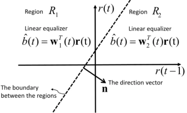
As an example, in Fig. 3, we use the received signal r(t) ≜

[r(t)

,

r(t

−

1)

]

T

_∈

R2to estimate the transmitted bit b(t). We partition the space R2_{into two regions w}

1

∈

R2and w2

∈

R2 in these regions respectively. Hence the estimateb(t) is calculated

ˆ

as

ˆ

b(t)

=

{

wT 1(t)r(t)

+

c1(t) if r(t)

∈

R1 w₂T(t)r(t)

+

c2(t) if r(t)

∈

R2

,

Fig. 3. A simple two region partition of the spaceR2. We use different equalizers w1and w2in regions R1and R2respectively. The direction vector n is an orthogonal vector to the regions boundary (the hyper-plane used to separate the regions).

where c1(t)

∈

R and c2(t)

∈

R are the offset terms, which can be embedded into w1and w2, i.e., wj ≜

[

wjT cj

]

T

,

j

=

1

,

2, and r≜

[

rT ₁

_]

T_{. Hence the above expression can be rewritten as}

ˆ

b(t)

=

{

wT 1(t)r(t) if r(t)

∈

R1 w₂T(t)r(t) if r(t)

∈

R2

.

We then update the equalizer’s coefficients using the LMS algo-rithm as

w1(t

+

1)

=

w1(t)

+

µ

1e(t) r(t) if r(t)

∈

R1 w2(t

+

1)

=

w2(t)

+

µ

2e(t) r(t) if r(t)

∈

R2

.

Note that, in our method (which will be discussed in the next section), we use LMS-based methods instead of other adaptive methods such as recursive least squares (RLS)-based methods due to the computational complexity constraints arising from running several different filters in parallel. However, one can straightfor-wardly extend our algorithm to use any other adaptive method.

To obtain a general expression, consider that we use a partition

P with N subsets (regions) to divide the space of the received signal

into disjoint regions, i.e., P

= {R

1

, . . . ,

RN

}

, Rh

= ∪

Nj=1Rj, and

ˆ

b(t)

= ˆ

bj(t)

=

wjT(t)r(t) if r(t)

∈

Rj, which can be rewritten using indicator functions as

ˆ

b(t)

=

N

∑

j=1

ˆ

bj(t) idj(r(t))

=

N

∑

j=1 w_jT(t)r(t) idj(r(t))

,

(2) where the indicator function idj(r(t)) determines whether r(t) lies in the region Rjor not, i.e., idj(r(t))

=

1 if r(t)

∈

Rj, and idj(r(t))

=

0 otherwise.

Remark 1. Note that this algorithm can be directly applied to

decision feedback equalizers (DFE). In this scenario, we partition the space of the extended received signal vector, i.e., we append the past decided symbols to the received signal vector asr(t)

˜

≜

[r(t)

, . . . ,

r(t

−

h

+

1)

, ¯

b(t

−

1)

, . . . , ¯

b(t

−

hf)

]

T, where hf is the length of the feedback part of the equalizer (i.e., we partition R(h+hf)). Also,b(t)

¯

=

Q (b(t)) denotes the quantized estimate of the

ˆ

transmitted bit b(t). Furthermore, corresponding to this extension in the received signal vector, we merge the feed-forward and feedback equalizers in each region to obtain an extended filter of length h

+

hfasw

˜

j(t)≜

[

wjT(t) fjT(t)

]

T, where fj(t) represents the feedback filter corresponding to the jth region at time t. Hence, the

jth region estimate is calculated asb

ˆ

j(t)

= ˜

wjT(t)r(t). In the next

˜

section, we extend these expressions to the case of an adaptive partition, both in the region boundaries and number of regions, and introduce our final algorithm.

3. Adaptive partitioning of the received signal space

3.1. An adaptive piecewise linear equalizer with a specific partition

Here, we consider a specific partition with a certain number of regions. However, due to the non-stationary nature of underwater channel, a fixed partitioning over time cannot match well to the channel response, i.e., the partitioning should be adaptive. Hence, we use a partition with adaptive boundaries, although the number of regions is still fixed. To this end, we use hyper-planes with adap-tive direction vectors (a vector orthogonal to the hyper-plane) as boundaries. Here, n to refers to the direction vector of a hyperplane. As an example, consider a partition with two regions (i.e., one boundary) as depicted inFig. 3. The indicator functions for these regions are calculated as id1(r(t))

=

σ

(r(t)) and id2(r(t))

=

1

−

σ

(r(t)), where

σ

(r(t))

=

1 if r(t)

∈

R1, and

σ

(r(t))

=

0 if r(t)

∈

R2, i.e.,

σ

(r(t)) represents the hard separation of the regions. However, in order to learn the region boundaries, we use a soft (differentiable) separator function, which is defined as

σ

(r)≜ 1 1

+

erT_n+b

,

(3) which yields

σ

(r)

=

{

1 if rTn

+

b

≪

0 0 if rTn

+

b

≫

0

which can be used to simply update the direction vector n using the LMS algorithm, resulting in an adaptive boundary. For simplicity, with a small abuse of notation, we redefine n and r, as n≜

[

nT _b]T and r≜

[

rT ₁

_]

T_{, hence(3)can be rewritten as}

_σ

_(r)

≜ 1

1+erT n. By using the LMS algorithm to update the direction vector n, n(t

+

1)

=

n(t)

−

1 2

µ ∇

n(t)e 2

=

n(t)

+

µ

e(t)

∂ ˆ

b(t)

∂

n(t)

=

n(t)

+

µ

e(t)

(

∂

id1(r(t))

∂

n(t)

ˆ

b1(t)

+

∂

id2(r(t))

∂

n(t)

ˆ

b2(t)

)

=

n(t)

+

µ

e(t)

σ

(r)(

σ

(r)

−

1)

(

_b

ˆ

_1(t)

_{− ˆ}

_b2(t)

)

_r(t)

_,

since

∂σ

(r)

∂

n

=

−

r erTn+b (1

+

erT_n+b₎2

= −

r

σ

(r)(1

−

σ

(r))

.

(4) Since the region boundaries as well as the linear filters in each region are adaptive, if every filter converges, this equalizer can perform better than other piecewise linear equalizers with the same number of regions.

Remark 2. The piecewise linear equalizers are not limited to the

BPSK modulation and one can easily extend these results to higher order modulation schemes like quadrature amplitude modulation (QAM) or pulse amplitude modulation (PAM). However, for the complex valued data (e.g., in QAM modulations) the separating function should change as

σ

(r) ≜ 1

1+exp[rTrenre+r_imTnim]

, where the subscripts ‘‘re’’ and ‘‘im’’ denote the real and imaginary part of each vector respectively.

3.2. The completely adaptive equalizer based on a turning boundaries tree

The block diagram of a sample adaptive piecewise linear equal-izer with adaptive regions is shown inFig. 4. Given a fixed number of regions, we can achieve the best piecewise linear equalizer with

Fig. 4. The block diagram of a turning boundaries tree (TBT) equalizer. The received

signal space is partitioned using a depth d tree, and corresponding to each node i there is a linear filter wi. Furthermore, the direction vectors of the separating hyper-planes, n’s, are adaptive resulting in an adaptive tree. The weight vector u, which contains the combination weights for each node’s contribution, is also adaptive.

the algorithm described in Section3.1. However, there is no a priori knowledge about the number of regions of the best piecewise linear equalizer, and the best linear equalizer will change in time, due to the highly non-stationary nature of underwater medium. In order to provide an acceptable performance with a relatively small computational complexity, we hierarchically partition the space of the received signal, i.e., Rh_{. Every node of the tree represents a} region and is fitted a linear equalizer, as shown inFig. 5. As shown inFig. 4, each node j provides its own estimateb

ˆ

j(t), which are then combined to generate the final estimate_{b(t) as}

ˆ

ˆ

b(t)

=

2d+1−1

∑

j=1 uj(t)wjT(t)r(t)

=

u T_(t)b(t)

ˆ

_,

₍₅₎

where u(t)

= [u

1(t)

, . . . ,

u2d+1−1(t)

]

Tis the combination weight vector, which is updated each time, and b(t)

ˆ

=

[ˆ

b1(t)

, . . . ,

ˆ

b₂d+1−1(t)

]

Tis the vector of the node estimates.

As depicted inFig. 6, this tree introduces a number of partitions with different number of regions, each of which can be separately used as a piecewise linear equalizer [16]. In our proposed tree structure, each node represents a region that is the union of the regions assigned to its left and right children [35], as shown in Fig. 5. The root node is denoted by 1, and the left and right children of the node j are denoted by 2j and 2j

+

1, respectively. Obviously the root node indicates the whole space of the received signal, i.e., Rh. The estimate generated by node j is calculated asb

ˆ

j(t)

=

wT

j(t) r(t). In addition,

α

drepresents the number of partitioning trees with depth

≤

d. Hence,

α

d+1

=

α

2d

+

1, which shows that there are a doubly exponential number of models embedded in a depth-d tree (SeeFig. 6), each of which can be used to construct a piecewise linear equalizer [30]. Each model consists of a number of nodes. However, the number of regions (leaf nodes) in each model can be different with that of other models, as shown inFig. 6, e.g., P2 has 2 regions, while P5 has 4 regions. Therefore, we implicitly run all of the piecewise linear equalizers constructed based on these partitions, and linearly combine their results to estimate the transmitted bit. Then, by adaptively learning the combination weights, we achieve the best estimate at each time.

To clarify, suppose the corresponding space of the received signal vector is two dimensional, i.e., r(t)

∈

_R2, and we partition this space using a depth-2 tree as inFig. 5. A depth-2 tree is represented by three separating functions

σ

1(r(t)),

σ

2(r(t)) and

σ

3(r(t)), which are defined using three hyper-planes with direction vectors n1(t), n2(t) and n3(t), respectively (SeeFig. 5). The left and

Fig. 5. Partitioning the spaceR2using a depth-2 tree structure. Hyper-planes (lines)

are used to divide the regions. The direction vectors are the orthogonal vectors to the hyper-planes.

Fig. 6. All different partitions of the received signal space that can be obtained using

a depth-2 tree. Any of these partition can be used to construct a piecewise linear equalizer, which can be adaptively trained to minimize the squared error. These partitions are based on the separation functions shown inFig. 5.

right children of the node j are 2j and 2j

+

1 respectively, therefore, the indicator functions are defined as

id1(r)

=

1 id2j(r)

=

σ

j(r)

×

idj(r) id2j+1(r)

=

(1

−

σ

j(r))

×

idj(r)

,

where j

≤

2d

−

1 and

σ

j(r)≜ 1 1+erT nj .

Due to the tree structure, three separating hyper-planes gen-erate four regions, each corresponding to a leaf node on the tree given inFig. 5. The partitioning is defined in a hierarchical manner, i.e., r(t) is first processed by

σ

1(r(t)) and then by

σ

i(t), i

=

2

,

3. A complete tree defines a doubly exponential number, O(22d

), of models each of which can be used to partition the space of the received signal vector. As an example, a depth-2 tree defines 5 different partitions as shown inFig. 6, each of which constructed using the leaves and the nodes of the original tree.

Consider the fifth model inFig. 6, i.e., P5, which consists of 4 disjoint regions, each corresponding to a leaf node of the original complete tree inFig. 5, labeled as 4, 5, 6, and 7. At each region, say the 4th_{region, we generate the estimateb}

ˆ

4(t)

=

wT4(t)r(t), where w4(t)

∈

Rh is the tap weights of the linear equalizer assigned to region 4. Considering the hierarchical structure of the tree and having calculated the region estimates,b

ˆ

j(t), the final estimate of

P5is given by

ˆ

b(5)(t)

=

7

∑

j=4 idj(r(t))b

ˆ

j(t)

,

(6)

for an arbitrary selection of the separator functions

σ

1

, σ

2

, σ

3and for any r(t). We emphasize that any Pi, i

=

1

, . . . ,

5 can be used in a similar fashion to construct a piecewise linear channel equalizer. Based on these model estimates, the final estimate of the transmitted bit b(t) is obtained by

ˆ

b(t)

=

αd

∑

i=1

ˆ

b(i)(t) u′_i(t)

= ˆ

b′(t)Tu′(t)

,

(7) where b

ˆ

′

(t) ≜

[ˆ

b(1)_(t)

_{, . . . , ˆ}

_b(αd)_(t)

_]

T _{and b}

ˆ

(k)_{(t) represents the} estimate of b(t) generated by the kth piecewise linear channel equalizer, k

=

1

, . . . , α

d. We use the LMS algorithm to update the weighting vector u′(t). Note that in our method, which is given in Algorithm 1, we linearly combine the estimates generated by all

α

d models, using the weighting vector u′

(t)≜

[u

′

1(t)

, . . . ,

u

′ αd(t)

]

T_{, to} estimate the transmitted bit b(t), such that we can achieve the best performance on the tree.

Under the moderate assumptions on the cost function that

e2_(u′

(t)) is a

λ

-strong convex function [36] and also its gradient is upper bounded by a constant number, the following theorem pro-vides an upper bound on the error performance of our algorithm (given in Algorithm 1).

Theorem 1. Let

{b(t)}

_t≥1 and

{r(t)}

t≥1 represents arbitrary and

real-valued sequences of transmitted bits and channel outputs. The algorithm forb(t) given in Algorithm 1 when applied to any sequence

ˆ

with an arbitrary length L

≥

1 yields

E

{

_L

∑

t=1

(

b(t)

− ˆ

b(t)

)

2

}

−

min z∈Rαd E

{

_L

∑

t=1

(

b(t)

−

zTb(t)

ˆ

)

2

}

≤

E

{

_L

∑

t=1

(

b(t)

− ˆ

b(t)

)

2

}

−

E

{

min z∈Rαd L

∑

t=1

(

b(t)

−

zTb(t)

ˆ

)

2

}

≤

O

(

log L

)

,

(8)

where z is an arbitrary constant combination weight vector, used to combine the results of all models.

Outline of the proof: Since we use a stochastic gradient method

to update the weighting vector in Algorithm 1, from Chapter 3 of [37]

it can be straightforwardly shown that

L

∑

t=1

(

b(t)

− ˆ

b(t)

)

2

−

min z∈Rαd L

∑

t=1

(

b(t)

−

zTb(t)

ˆ

)

2

≤

O

(

log L

)

,

in a strong deterministic sense, which is a well known result in computational learning theory [37]. Taking the expectation of both

sides of this deterministic bound yields the result in(8).

This theorem implies that the algorithm given in Algorithm 1 asymptotically achieves the performance of the optimal linear combination of the

α

d

≈

(1

.

5)2

d

different adaptive piecewise linear equalizers, represented using a depth-d tree, in the MSE sense, with a computational complexity O(h4d_{) (i.e., only polynomial in the}

number of nodes). Moreover, note that as the data length increases and each region becomes dense enough, the linear equalizer in each region, converges to the corresponding linear MMSE equalizer in that region [30]. In addition, since in our algorithm the tree structure is also adaptive, it can follow the data statistics effectively even when the channel is highly time varying. Therefore, our algo-rithm outperforms the conventional methods and asymptotically achieves the performance of the best piecewise linear equalizer.

By adjusting the combination weights using LMS algorithm to achieve the performance of the best piecewise linear equalizer we obtain

u′(t

+

1)

=

u′(t)

−

1

2

µ∇

u′(t)e 2_(t)

₌

_u′

(t)

+

η

e(t)b(t)

ˆ

.

Note that, as depicted inFig. 6, each model weight equals the sum of the weights assigned to its leaf nodes, hence, we have u′

k(t)

=

∑

i∈Pkui(t), which in turn results in the following node weights update algorithm

uj(t

+

1)

=

uj(t)

+

µ

e(t)b

ˆ

j(t) idj(r(t))

,

where uj(t) denotes the weight assigned to the jth node at time t. So far, we have shown how to construct a piecewise linear equalizer using separating functions and how to combine the es-timates of all models to achieve the performance of the best piece-wise linear equalizer. However, there are a doubly exponential number of these models, hence it is computationally prohibited to run all of these models and combine their results. In order to reduce this complexity while reaching exactly the same result, we directly combine the node estimates, i.e., instead of running all possible models, we combine the node estimates with special weights, which yields the same result. We now illustrate how to directly combine the node weights in our algorithm. The overall estimate using all models contributions is

ˆ

b(t)

=

αd

∑

i=1

ˆ

b(i)_{(t) u}′ i(t)

=

αd

∑

i=1

ˆ

b(i)(t)

⎛

⎝

∑

j∈Pi uj(t)

⎞

⎠

=

αd

∑

i=1

⎛

⎝

∑

k∈Pi idk(r(t))b

ˆ

k(t)

⎞

⎠

⎛

⎝

∑

j∈Pi uj(t)

⎞

⎠

=

αd

∑

i=1

⎛

⎝

∑

j,k∈Pi idk(r(t))b

ˆ

k(t)uj(t)

⎞

⎠

,

(9)

where j and k indicate two arbitrary nodes. For each node k, we define zk(t) ≜ idk(r(t)) b

ˆ

k(t). Hence we have b(t)

ˆ

=

∑

αd i=1

(

∑

j,k∈Pizk(t)uj(t)

)

.

Consider thatΓ

= {

Γ1

, . . . ,

Γθd(dk)

}

is the family of models (subtrees) in all of which the node k is a leaf node, where

θ

d(dk) denotes the number of such models. Therefore the final estimate of our algorithm can be rewritten as:

ˆ

b(t)

=

2d+1−1

∑

k=1 zk(t)

⎡

⎣

∑

j∈_Γ1 uj(t)

+ · · · +

∑

j∈_Γθ d (dk ) uj(t)

⎤

⎦

.

We denote by

ρ

(j0

,

k) the number of models in all of which the nodes j0and k appear as the leaf nodes simultaneously. The weight of each node j0(i.e., uj0) appears in the above expression

exactly

ρ

(j0

,

k) times, which yields the following expression for the final estimate _b(t)

ˆ

₌

∑

2d+1−1

k, none of the children of that is a common ancestor of j and k.

This parameter can be calculated using the following algorithm. Assume that, without loss of generality, j

≤

k. Obviously if j is an

ancestor of k, it is also the nearest common ancestor, i.e., l

=

dj. However, if j is not an ancestor of k, we define j′≜ 2dk−dj_{j, which} is a grandchild of the node j. Hence, the nearest common ancestor of j′

and k is that of j and k. The following procedure computes the parameter l. l

=

0;

δ =

dk; while (l

≤

dk) do

δ = δ −

l; if (j′

_,

k

≤

2δ−1

+

2δor j′

_,

k

≥

2δ−1

+

2δ) then l

=

l

+

1; else stop; end end

In order to update the region boundaries, we update their direction vectors as follows

nj(t

+

1)

=

nj(t)

−

1 2

µ∇

nj(t)e

2_(t)

_,

₍₁₀₎

where

∇

_nj(t)e2_{(t) is the derivative of e}2_{(t) with respect to n} j(t). Since e(t)

=

b(t)

− ˆ

b(t) the updating expression can be calculated

as follows nj(t

+

1)

=

nj(t)

−

1 2

µ∇

nj(t)e 2_(t)

=

nj(t)

+

µ

e(t)

∂ ˆ

b(t)

∂

nj(t)

=

n_j(t)

+

µ

e(t) 2d+1₋₁

∑

k=1

∂ ˆ

b(t)

∂

zk(t)

∂

zk(t)

∂

n_j(t)

=

nj(t)

+

µ

e(t) 2d+1−1

∑

k=1

β

k(t)b

ˆ

k(t)

∂

idk(r(t))

∂

nj(t)

=

nj(t)

+

µ

e(t) 2d+1−1

∑

k=1

β

k(t)b

ˆ

k(t)

∂

idk(r(t))

∂ σ

j(r(t))

∂ σ

j(r(t))

∂

nj(t)

=

nj(t)

+

µ

e(t)

∂ σ

j(r(t))

∂

nj(t) 2d+1−1

∑

k=1

β

k(t)b

ˆ

k(t)

∂

idk(r(t))

∂ σ

j(r(t))

.

However note that not all of the idk(r(t)) functions involve

σ

j(r(t)), i.e., only the nodes of the subtree with the root node j are included.

s=2m

σ

j(r(t))

We have presented the Algorithm 1 for a ‘‘turning boundaries tree’’ (TBT) equalizer, which is completely adaptive to the channel response. Especially in our algorithm both the number of regions and the region boundaries as well as the linear equalizers in each region are adaptive. We emphasize that the learning rates and initial values of all filters can be different.

3.3. Complexity

Consider that we use a depth-d tree to partition the space of the received signal, Rh_{. First note that each node estimate needs h} computation. Since we update all the linear filters corresponding to each region at each specific time, it generates a computational complexity of O(h(2d+1

₋

_{1)). Also, updating the separator functions} results in a computational complexity of O(h(2d

₋

_{1)). Moreover,} note that we compute the cross-correlation of every node esti-mate and every node weight, which results in the complexity of

O(hN2

d)

=

O(h4d). Hence, our algorithm has the complexity O(h4d), which is only polynomial in the number of the tree nodes.

4. Simulations

We show the efficacy of our algorithm (TBT) over a synthetic and a real world acoustic channel and compare our algorithm to state-of-the-art equalization methods including: the Fixed Bound-aries Tree (FBT) equalizer, Finest Partition with Fixed BoundBound-aries (FF), Finest Partition with Turning Boundaries (FT) (all having depths d

=

2), linear normalized LMS (NLMS) equalizer, Variable Step Size LMS (VSLMS) of [38], and Subband Adaptive Filter [39]. In addition, we implement and compare the performance of our al-gorithm and the NLMS in a DFE structure, denoted by DFE-TBT and DFE-NLMS, respectively. The Finest Partition refers to the partition consisted of all leaf nodes of the tree (the P5model inFig. 6). Also, we use FBT to refer to an equalizer with ‘‘fixed’’ boundaries, which adaptively update the node weights as well as TBT algorithm. We use the LMS algorithm in the linear equalizer of each node for all algorithms. For the direction vector at node j, i.e., nj, we set the dj-th element to 1, and all other elements to zero, where djindicates the depth of this node on the tree. All other filters are initialized by all zero vectors

4.1. Experiments on a simulated channel 4.1.1. Setup

In this section, we illustrate the performance of our algorithm under a highly realistic UWA channel equalization scenario. The UWA channel response is generated using the algorithm intro-duced in [40], which presents highly accurate modeling of the real life UWA communication experiments. The simulation con-figurations and the parameters used for simulating the channel are presented in the Table 1. We sent 60000 bits generated by

Compute

ρ

(j

,

k) for all pairs

{j

,

k}of nodes; for t

=

1 to L do r

= [r(t)

, . . . ,

r(t

−

h

+

1)

]

T_; for k

=

1 to 2d

₋

_{1 do}

σ

k

=

1 1+erT nk ; end id1

=

1; for k

=

1 to 2d

−

1 do id2k

=

idk

σ

k; id2k+1

=

idk(1

−

σ

k); end

ˆ

b

=

0; for k

=

1 to 2d+1

₋

_{1 do}

ˆ

bk

=

wkTr; zk

= ˆ

bkidk;

β

k

=

0; for j

=

1 to 2d+1

₋

_{1 do}

β

k

=

β

k

+

uj

ρ

(j

,

k); end

ˆ

b(t)

= ˆ

b(t)

+

zk

β

k; end

if train mode then

¯

b

=

b(t); else

¯

b

=

Q (b(t));

ˆ

end e

= ¯

b

− ˆ

b(t); for k

=

1 to 2d+1

−

1 do wk

=

wk

+

µ

ke idkr; uk

=

uk

+

η

e zk; end for j

=

1 to 2d

₋

_{1 do} dj

= ⌊

log2(j)

⌋

; for m

=

0 to d

−

dj

−

1 do for p

=

0 to 2m

₋

_{1 do} i

=

2m+1_j

₊

_p; S1

=

S1

+

β

ib

ˆ

i id_σji; end for p

=

2mto 2m+1

−

1 do i

=

2m+1_j

₊

_p; S2

=

S2

+

β

ib

ˆ

i id_σji; end S

=

S

+

S1

−

S2; end n_j

=

n_j

+

ζ

_je

σ

(

σ −

1) S r; end end

Algorithm 1: Turning Boundaries Tree (TBT) Equalizer

repeating a Turyn sequence [41] (with a length of 28 bits), after pulse shaping with a raised cosine filter with a roll-off factor of 0.25, over the simulated UWA channel shown inFig. 7. In addition, the system setup is the same as one described at Section2.2. Also, we have calculated the SNR after down converting and matched filtering (i.e., from the baseband signal). The step sizes are set to

µ =

0

.

08 for all equalizers except the SAF, which has a step size of 0.01. Furthermore, in SAF we use 4 subbands, in all of which we use the same step size. In all algorithms we have used length 5 equalizers. Also, the length of feedback part in DFEs is set to 3. The

Fig. 7. Time evolution of the magnitude baseband impulse response of the

gener-ated channel [40].

Table 1

The simulated channel configurations.

Parameters Values

Depth 100 m

Tx height 20 m

Rx height 50 m

Distance between Tx and Rx 1 km

Carrier Frequency (fc) 10.8 kHz

Bandwidth 1.6 kHz

Minimum frequency (fmin) 10 kHz

Frequency resolution (df ) 100 Hz

Time resolution (dt) 10/16 ms

Coherence time of the small scale variants (TSS) 60 s Total duration of simulated channel (Ttot) 60 s

results are averaged over 10 repetitions, and show the extremely superior performance of our algorithm over other methods

4.1.2. Results and discussion

Fig. 8bshows the normalized time accumulated squared errors

of the equalizers, when SNR

= −

5 dB. We emphasize that the TBT equalizer significantly outperforms its competitors, where the FBT equalizer cannot provide a satisfactory result at the low SNRs, since it commits to the initial partitioning structure. Note that the TBT equalizer adapts its region boundaries and can successfully per-form channel equalization even for a highly difficult UWA channel. TheFig. 8ashows the bit error rate performance in different SNRs for different equalizers.

In the second experiment, again, we sent 60000 symbols of repeated Turyn sequence over the simulated channel and used TBT algorithm with different depths to equalize the channel. The results, as shown inFig. 9, demonstrate that increasing the depth of the tree improves the performance. However, as the depth of the tree increases, the effect of the depth diminishes. This is because increasing the depth introduces finer partitions, i.e., the partitions with more regions. As the number of the regions in a partition increases, the data congestion in each region decreases, hence, the linear filters in these regions cannot fully converge to their MMSE solutions. As a result, the estimates of these regions (nodes) will be contributed to the final estimate with a much lower combination weight than other nodes, which are also present in a lower depth tree. Therefore, although increasing the depth of the tree improves the result, we cannot get a significant improvement in the performance by only increasing the depth.

(a) The BER comparison.

(b) The MSE comparison.

Fig. 8. The BER and MSE comparison for different equalizers in the synthetic

channel [40] experiment.

Fig. 9. The MSE performance comparison for different depths TBT equalizers at

SNR= −5 dB.

Fig. 10. The evolution of node combination weights in TBT algorithm, in the

synthetic channel experiment, at SNR= −5 dB.

Moreover, the evolution of node combination weights in the synthetic channel [40] experiment is shown inFig. 10, which indi-cates the contribution of each node’s estimate in the final estimate. This figure shows that node 1, the root node, has the largest weight at the early stages of the algorithm, while its weight decreases as the time passes. On the other hand, the weights assigned to nodes with finer partitions, e.g., nodes 4, 6, and 7, gradually increase. Therefore, as the finer models receive sufficient amount of data to be trained with, they contribute more to the final nonlinear estimation.

4.2. Experiments on a real world dataset

To evaluate the efficacy of our algorithm in a real life scenario, we use a dataset provided by the Applied Research Laboratory (ARL) at University of Texas-Austin, on November 2009 [42,43]. The maximum depth of the lake is about 37 meters. The distance between the transmitter and the receiver is in range of 73

−

267 meters, and there is a towing motion of the transducer at speeds of

∼

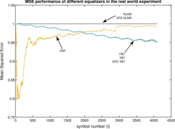
5 km/h at varying depths of at most 5 m [42].

We use one of the packets described in this dataset, which consists of 4096 BPSK modulated symbols which are later pulse shaped by a raised cosine filter with a roll-off factor of 1. Also, the first 52 symbols of the transmitted data frame, is consisted of 4 repetitions of a Barker sequence of length 13. The power spectrum of the transmitted and received signals are depicted inFig. 11. The sampling rate at the transmitter and receiver is 200 kHz, the symbol rate is 15.625 kHz, and the carrier frequency is 62.5 kHz. We have set the step size of all methods to 0.0001, the depth of trees to 2, and the number of subbands in SAF method to 16.

The receiver consists of a frame synchronizer block such that it receives a base banded packet of the data, searches for four consec-utive blocks of Barker sequence each of length 13, which precedes the data frame. Then, the data frame passes through the Doppler compensation filter (discussed in Section2.3) and is resampled at a rate of 4 samples per symbol. Finally, the equalizer removes the ISI effect from the data.Fig. 12shows the MSE performances of different equalizers on the described dataset. Furthermore, the Table 2indicates the resulting bit error rates using each equalizers. As depicted inFig. 12andTable 2, our method significantly outper-forms the other methods in this real life experiment. Moreover, as

Table 2

The BER performance of different methods over the ARLUT dataset.

Algorithm NLMS DFE-NLMS VSLMS SAF FBT TBT DFE-TBT

BER 0.5112 0.5068 0.4880 0.3447 0.2976 0.2903 0.2971

Fig. 11. The power spectrum of the transmitted and received signals in ARLUT

dataset, obtained using ‘‘Welch’’ method in MATLAB.

Fig. 12. The MSE performance comparison of different methods in the experiment

over ARLUT dataset.

shown by the figure, the tree based methods provide the best MSE convergence performance, while the conventional NLMS method and its DFE counterpart fail to deliver an acceptable performance.

5. Conclusion

We study nonlinear UWA channel equalization using hierarchi-cal structures, where we partition the received signal space using a nested tree structure and use different linear equalizers in each region. In this framework, we introduce a tree based piecewise linear equalizer that both adapts its linear equalizers in each region

as well as its tree structure to best match to the underlying channel response. Our algorithm asymptotically achieves the performance of the best linear combination of a doubly exponential number of adaptive piecewise linear equalizers represented on a tree with a computational complexity only polynomial in the number of tree nodes. Since our algorithm directly minimizes the squared error and avoid using any artificial weighting coefficients, it strongly outperforms the conventional linear and piecewise linear equal-izers as shown in our experiments.

Acknowledgments

This work is in part supported by Turkish Academy of Sci-ences, Outstanding Researcher Programme, and TUBITAK, Contract No:112E161.

References

[1] B. Xerri, J.-F. Cavassilas, B. Borloz, Passive tracking in underwater acoustic, Signal Process. 82 (8) (2002) 1067–1085. http://dx.doi.org/10.1016/S0165-1684(02)00240-2.

[2] A.C. Singer, J.K. Nelson, S.S. Kozat, Signal Process. for underwater acoustic communications, IEEE Commun. Mag. 47 (1) (2009) 90–96.

[3] D.B. Kilfoyle, A.B. Baggeroer, The state of the art in underwater acoustic telemetry, IEEE J. Ocean. Eng. 25 (1) (2000) 4–27.http://dx.doi.org/10.1109/ 48.820733.

[4] J.W. Choi, T.J. Riedl, K. Kim, A.C. Singer, J.C. Preisig, Adaptive linear turbo equalization over doubly selective channels, IEEE J. Ocean. Eng. 36 (4) (2011) 473–489.

[5] M. Stojanovic, Recent advances in high-speed underwater acoustic communi-cations, IEEE J. Ocean. Eng. 21 (2) (1996) 125–136.

[6] J.C. Patra, P.K. Meher, G. Chakraborty, Nonlinear channel equalization for wire-less communication systems using legendre neural networks, Signal Process. 89 (11) (2009) 2251–2262.http://dx.doi.org/10.1016/j.sigpro.2009.05.004. [7] H. Zhang, Y. Shi, A. Saadat Mehr, H. Huang, Robust FIR equalization for

time-varying communication channels with intermittent observations via an LMI approach, Signal Process. 91 (7) (2011) 1651–1658.

[8] N. Iqbal, A. Zerguine, N. Al-Dhahir, Decision feedback equalization using par-ticle swarm optimization, Signal Process. 108 (Complete) (2015) 1–12.http: //dx.doi.org/10.1016/j.sigpro.2014.07.030.

[9] Y. Zhang, J. Zhao, Y. Guo, J. Li, Blind adaptive MMSE equalization of underwater acoustic channels based on the linear prediction method, J. Mar. Sci. Appl. 10 (1) (2011) 113–120.http://dx.doi.org/10.1007/s11804-011-1050-9. [10]S. Fki, M. Messai, A. Aissa El Bey, T. Chonavel, Blind equalization based on pdf

fitting and convergence analysis, Signal Process. 101 (2014) 266–277. [11] A. Radosevic, T. Duman, J. Proakis, M. Stojanovic, Channel prediction for

adaptive modulation in underwater acoustic communications, in: OCEANS, 2011 IEEE — Spain, 2011, pp. 1–5.http://dx.doi.org/10.1109/Oceans-Spain. 2011.6003438.

[12] A. Song, M. Badiey, Generalized equalization for underwater acoustic commu-nications, in: Proceedings of OCEANS 2005 MTS/IEEE, 2005, pp. 1522–1527. http://dx.doi.org/10.1109/OCEANS.2005.1639971.

[13]K. Yeo, K. Pelekanakis, M. Chitre, Time-domain equalization for underwa-ter acoustic OFDM systems with insufficient cyclic prefix, in: OCEANS’11 MTS/IEEE KONA, 2011, pp. 1–5.

[14]B. Li, S. Zhou, M. Stojanovic, L. Freitag, P. Willett, Multicarrier communication over underwater acoustic channels with nonuniform doppler shifts, IEEE J. Ocean. Eng. 33 (2) (2008) 198–209.

[15]M. Stojanovic, J. Preisig, Underwater acoustic communication channels: Prop-agation models and statistical characterization, IEEE Commun. Mag. 47 (1) (2009) 84–89.

[16]N.D. Vanli, S.S. Kozat, A comprehensive approach to universal piecewise non-linear regression based on trees, IEEE Trans. Signal Process. 62 (20) (2014) 5471–5486.

[17]K. Kim, N. Kalantarova, S.S. Kozat, A.C. Singer, Linear MMSE-optimal turbo equalization using context trees, IEEE Trans. Signal Process. 61 (12) (2013) 3041–3055.

[18] Y. Xiao, F. liang Yin, Blind equalization based on RLS algorithm using adaptive forgetting factor for underwater acoustic channel, China Ocean Eng. 28 (3) (2014) 403–408.http://dx.doi.org/10.1007/s13344-014-0032-5.

[23]M. Meyer, G. Pfeiffer, Multilayer perceptron based decision feedback equalis-ers for channels with intequalis-ersymbol interference, IEE Proceedings I (Communi-cations, Speech and Vision) 140 (4) (1993) 420–424.

[24] H. Zhao, J. Zhang, Functional link neural network cascaded with chebyshev orthogonal polynomial for nonlinear channel equalization, Signal Process. 88 (8) (2008) 1946–1957http://dx.doi.org/10.1016/j.sigpro.2008.01.029. URL http://www.sciencedirect.com/science/article/pii/S0165168408000480. [25] J.C. Patra, R.N. Pal, A functional link artificial neural network for adaptive

channel equalization, Signal Process. 43 (2) (1995) 181–195http://dx.doi.org/ 10.1016/0165-1684(94)00152-P.

[26] A. Pradhan, S. Meher, A. Routray, Communication channel equalization us-ing wavelet network, Digital Signal Process. 16 (4) (2006) 445–452http: //dx.doi.org/10.1016/j.dsp.2005.06.001. URL http://www.sciencedirect.com/ science/article/pii/S1051200405000953.

[27] Q. Gan, P. Saratchandran, N. Sundararajan, K.R. Subramanian, A complex valued radial basis function network for equalization of fast time varying channels, IEEE Trans. Neural Netw. 10 (4) (1999) 958–960.http://dx.doi.org/ 10.1109/72.774271.

[28] H. Jiang, K.S. Kwak, Recurrent neural network adaptive equalizers based on data communication, J. Commun. Netw. 5 (1) (2003) 7–18.http://dx.doi.org/ 10.1109/JCN.2003.6596681.

[29] J. Choi, A.C.C. Lima, S. Haykin, Kalman filter-trained recurrent neural equalizers for time-varying channels, IEEE Trans. Commun. 53 (3) (2005) 472–480.http: //dx.doi.org/10.1109/TCOMM.2005.843416.

[30]S.S. Kozat, A.C. Singer, G.C. Zeitler, Universal piecewise linear prediction via context trees, IEEE Trans. Signal Process. 55 (7) (2007) 3730–3745.

[31] O.J.J. Michel, A.O. Hero, A.-E. Badel, Tree-structured nonlinear signal modeling and prediction, IEEE Trans. Signal Process. 47 (11) (1999) 3027–3041.http: //dx.doi.org/10.1109/78.796437.

[32] S. Gelfand, C. Ravishankar, E. Delp, Tree-structured piecewise linear adaptive equalization, IEEE Trans. Commun. 41 (1) (1993) 70–82.http://dx.doi.org/10. 1109/26.212367.

[33]F. Qu, L. Yang, Basis expansion model for underwater acoustic channels?, in: OCEANS 2008, 2008, pp. 1–7.

[34]A.H. Sayed, Fundamentals of Adaptive Filtering, John Wiley & Sons, NJ, 2003. [35] F.M.J. Willems, Y.M. Shtarkov, T.J. Tjalkens, The context-tree weighting method:

basic properties, IEEE Trans. Inform. Theory 41 (3) (1995) 653–664.http: //dx.doi.org/10.1109/18.382012.

[36]E. Hazan, A. Agarwal, S. Kale, Logarithmic regret algorithms for online convex optimization, Mach. Learn. 69 (2–3) (2007) 169–192.

[37]N. Cesa-Bianchi, G. Lugosi, Prediction, Learning, and Games, Cambridge Uni-versity Press, New York, NY, USA, 2006.

[38] J.K. Hwang, Y.P. Li, Variable step-size LMS algorithm with a gradient-based weighted average, IEEE Signal Process. Lett. 16 (12) (2009) 1043–1046.http: //dx.doi.org/10.1109/LSP.2009.2027653.

[39] J.J. Shynk, Frequency-domain and multirate adaptive filtering, IEEE Signal Process. Mag. 9 (1) (1992) 14–37.http://dx.doi.org/10.1109/79.109205. [40]P. Qarabaqi, M. Stojanovic, Statistical characterization and computationally

efficient modeling of a class of underwater acoustic communication channels, IEEE J. Ocean. Eng. 38 (4) (2013) 701–717.

Polytechnic), Tehran, Iran, July 2014. He is currently an M.S. student at the Department of Electrical and Electron-ics Engineering, Bilkent University, Ankara, Turkey. His current research interests include learning theory, online learning, big data analytics, optimization, statistical signal processing, and adaptive filtering.

Nuri Denizcan Vanli received the B.S. and M.S. degrees

in electrical and electronics engineering from Bilkent Uni-versity, Ankara, Turkey, in 2013 and 2015, respectively. He is currently working toward the Ph.D. degree in electrical engineering and computer science at Massachusetts Insti-tute of Technology, Cambridge, MA, USA. His research in-terests include convex optimization, online learning, and distributed optimization.

Suleyman Serdar Kozat (A’10–M’11–SM’11) received the

B.S. degree with full scholarship and high honors from Bilkent University, Turkey. He received the M.S. and Ph.D. degrees in electrical and computer engineering from Uni-versity of Illinois at Urbana–Champaign, Urbana, IL. Dr. Kozat is a graduate of Ankara Fen Lisesi. After graduation, Dr. Kozat joined IBM Research, T. J. Watson Research Lab, Yorktown, New York, US as a Research Staff Member in the Pervasive Speech Technologies Group. While doing his Ph.D., he was also working as a Research Associate at Microsoft Research, Redmond, Washington, US in the Cryptography and Anti-Piracy Group. He holds several patent inventions due to his research accomplishments at IBM Research and Microsoft Research. Dr. Kozat is currently an Associate Professor at the Electrical And Electronics Engineering Department of Bilkent University. Dr. Kozat is the President of the IEEE Signal Processing Society, Turkey Chapter. He has been elected to the IEEE Signal Process. Theory and Methods Technical Committee and IEEE Machine Learning for Signal Process. Technical Committee, 2013. He has been awarded IBM Faculty Award by IBM Research in 2011, Outstanding Faculty Award by Koc University in 2011 (granted the first time in 16 years), Outstanding Young Researcher Award by the Turkish National Academy of Sciences in 2010, ODTU Prof. Dr. Mustafa N. Parlar Research Encouragement Award in 2011, Outstanding Faculty Award by Bilim Kahramanlari, 2013 and holds Career Award by the Scientific Research Council of Turkey, 2009.