Absence of phase transitions in one-dimensional antiferromagnetic models with long-range interactions

Journal o f Statistical Physics, Vol. 72, Nos. 3/4, 1993

Absence of Phase Transitions in

One-Dimensional Antiferromagnetic Models

with Long-Range Interactions

A z e r K e r i m o v 1, 2

Received August 4, 1992; final April 16, 1993

The absence of phase transitions in a one-dimensional model with long-range antiferromagnetic potential is established at low temperatures when the ground states have a rational density. A description of the set of all ground states and typical configurations is given.

KEY W O R D S : Hamiltonian; ground state; Gibbs state; interacting and noninteracting contours; extreme Gibbs state.

1. I N T R O D U C T I O N

We consider a classical lattice model of statistical mechanics on a one- dimensional lattice, the spin variable q~(x) at each point x taking the values 0 and 1. The interaction is specified by means of the Hamiltonian

I-I(~o(x))=

y~

U(x-y)~o(x)~o(y)-~ y~ ~o(x)

(1)

x, y E Z l ; x > y x ~ Z 1

where # is the external field. The following conditions are imposed on the potential U(x):

1. U ( x ) > 0 at x ~ Z 1, x > 0 . 2. Zx~z~ U(x)< ~ .

3. U ( x + y ) + U ( x - y ) > 2 U ( x ) ; x, y ~ Z 1, x > y .

t Depmartment of Mathematics, Bilkent University, 06533 Bilkent, Ankara, Turkey. 2 Permanent address: Institute of Mathematics and Mechanics, Academy of Sciences of

Azerbaijan, Baku 370602, Azerbaijan.

571

4. The function U(x) can be extended to a twice continuously

differentiable function such that U ( x ) ~ A x -~, U ' ~ - A v x ~-1, and

U"(x) ~ AT(y + 1 ) x - ~ - 2 at x ~ 0% where ~ > 1, and A is a strong positive

constant.

The first condition means that the model (1) is antiferromagnetic. The natural second condition is necessary for the existence of the thermo- dynamic limit. The third condition on the convexity of the interaction function U(x) is essential for all further evaluations. The fourth condition

determines the character of the potential's decrease at infinity.

The main purpose of the present paper is to investigate the structure of the set of all Gibbs states (1) of the model (1).

The hypothesis on the uniqueness of the Gibbs states in the model (1) was stated by Sinai in 1983 (see ref. 2, Problem 1).

It is well known that the condition Zx~zl,x>0 x U ( x ) < oo automati-

cally implies the uniqueness of the Gibbs states. (3-5) Therefore, we investigate the problem of the phase transitions in the model (1) for potentials U(x) ~ Ax -~, where 7 = 1 + ~, 0 < c~ < 1. The ferromagnetic case

[when the potential U(x) is negative] was considered by Dyson. (6'7) He

considered a model with the following potential [the external field is absent, spin variable ~o(x) takes the values + 1 , - 1 ] :

1. U(x) < O.

2. Zx~zl lU(x)l < oo. 3. U(x + 1) > U(x).

4. Zx~Z~x>olnln(x+4) - l x 3 U ( x ) -~< oo.

Note that all potentials decreasing as x -1-~, O<c~< 1, certainly satisfy the above conditions.

Dyson established that in the ferromagnetic case one can find/~1 such that if fl > / ~ then there exist at least two extremal Gibbs states P+ and P - corresponding to the ground states q~(x)= +1 and r - 1 . This very profound result is connected with the following fact. Let us consider the boundary conditions q3(x)= 1, the segment I - - n , n], and the configuration

~0 l(X) such that q)_1(x) = - 1 if x e [ - n , n], and q ) l ( X ) = 1 if x e Z 1 -

I - n , n]. Then the difference between the energies of the configurations q~ ~(x) and qS(x) is of order n t-~. In other words, in the one-dimensional case there arises an analog of the notion of the surface tension and this fact leads to the existence of two extremal Gibbs states, as could be anticipated. In the antiferromagnetic case we are faced with a quite different situation. It will be shown that at arbitrary fixed boundary conditions qS(x), x e Z 1 - I - - n , n], a configuration cp(x), x e l - - n , n], with maximal

Absence of Phase Transitions in 1 D AF M o d e l s 573

weight (or with minimal energy) almost does not differ from the special ground state with the exception of some bounded zone and is stable in the sense of Peierls (see Lemma 5). This fact has a decisive significance in establishing all further results.

A series of papers has been devoted to the investigation of the ground states of the model (i)/8-1~ 1 1 - 1 4 )

Let us now briefly introduce necessary definitions and facts. Let #per denote the set of all periodic configurations. F o r every ~0 ~ ~b per we define

q-~y=x+l-vx+P q~(x)/p,

where p is the period of q~. It is obvious that q does not depend on x. Therefore, the density of each periodic configuration is

= q/p.

It is more convenient to work with the reciprocal of the density, ~/(~0(x)) =

p/q,

which represents the average distance between neighboring points at which q~(x)= 1. F o r every configuration ~o E q~per we define the mean energy h(~0) as follows:

1 x + p

= -

Z

q (x) U(z) o(y + z)

Py=x+l

z > 0

It is readily seen that this expression is independent of x.

The special definition of the ground state was formulated in ref. 2. This definition does not coincide with the generally accepted one (1) and is useful for describing the phase diagram of the model (1) at zero temperature.

Let p/q be a fixed positive rational number.

Definition 1 .(2) A configuration ~0o(X ) e t~ per with

q(~Oo(X ) = p/q)

is called a special ground state if

h(q~(x))

= inf h(~0)

~p e ~Per, r/(q~) = p/q

The following proposition readily follows from the convexity of the potential

U(x).

Hubbard's C r i t e r i o n . (2"8) Let ~0 e Cper and let

ri(x; ~o)

denote the distance between x e Z ~ and the ith particle on the right. If for each x and i

[#/] ~<

r~(x; q~)<. [in] + 1

(the square brackets denote the integral part of the enclosed number) then ~o is a special ground state.

The existence of a configuration satisfying Hubbard's criterion (the special ground state) is proved in ref. 2. A remarkable short formula for the special ground states was given by S. Aubry (see ref. 13). Here we give the construction of the special ground state for each fixed rational

value of the density s:. (z) Special g r o u n d states for irrational densities are investigated in refs. 13 a n d 14.

Every rational n u m b e r p/q can be uniquely d e c o m p o s e d into a finite

c o n t i n u e d fraction. We write it as p/q = [-no, nl ... ns], which means

1

n o + 1

n l + 1

n z + - . - + - -

r/s

The g r o u n d state for a configuration with s: = [-no, nl ... ns] will be constructed by induction.

1. ~C=no~>l, nl is an integer. It is then obvious that a periodic configuration with equally distant x at which ~o(x)= 1 satisfies H u b b a r d ' s

criterion, i.e., is a special g r o u n d state. In this case ri(x; q~)= ino, i > 0 .

2. ~: = n o + 1/nl, where n o and n 1 are integers, no ~> 1, n l > 1. T h e n the

(non1 + 1)-periodic configuration

0 ... 0 1 0 ... 01 ... 0 ... 01

n o + 1 n o n o n l -- 1 t i m e s

also satisfies H u b b a r d ' s criterion a n d is a special g r o u n d state.

3. • = [no, nl,..., ns], where no, nl,..., ns are integers, no, nl,..., ns >/1.

F o r s = 0 a n d s = 1 the required configurations are already constructed.

Suppose we have already c o n s t r u c t e d a g r o u n d state with s = m a n d

~:= [no, nl,...,nm]. T h e n the following configuration with s = m + 1 and

K' = [ - n O , F/1 . . . n m + l ] is constructed:

~O(no,..., nm+ 1) - - ~0(/'/0,'", /~/m 1) ~O(no ... nm)"" q~(no ... Plrn) nm + 1 times

Here, 9(n0,..., nj), j = m - 1 , m, m + 1, are the blocks f r o m which the

g r o u n d states for ~ = [-no,..., nj] are obtained by periodic continuations.

(2)

It can be verified that the constructed configuration satisfies H u b b a r d ' s

criterion a n d therefore is a special g r o u n d state for tc = [no, n l ... nm, nm+ 1].

H u b b a r d ' s criterion allows us to extract an explicit expression for the m e a n energy of a special g r o u n d state(Z):

h~= ~ ~ U(mi) ~U+ U(m,+ 1)(1 - z c ; ) (2)

i = 1

Absence of Phase Transitions in 1D AF Models 575

This formula shows that the function of mean energy is continuous on the set of all rationals and can be extended to a continuous function defined on the whole segment [0, + oe).

T h e o r e m 1 .(2,10) 1. The function h~ is convex.

2. In each rational point the function h~ has a left-hand derivative #~ and a right-hand derivative # ~ , w i t h / ~ > / ~ - . + +

3. The Lebesgue measure of the complement of the set U~ (#~-, / t+) in the real line R is zero.

T h e o r e m 2. (u) Suppose that the value of the external field/~ of the model (1) belongs to the interval ( / ~ , / ~ + ) for some number ~c = q/p. Then the special ground state of the model (1) is unique to within a translation. In this paper we establish the validity of Sinai's hypothesis at low temperatures almost (with respect to the Lebesgue measure) for each value of the external field. The main result of the present paper (and the solution of Problem 1 of ref. 2 almost for each value of the external field) is the following:

T h e o r e m 3. Suppose that the value of the external field # of the

model (1) belongs to the interval (/tK, #+ ) for some number ~ = q/p.

Then the model (1) has a unique Gibbs state at all sufficiently small values of the temperature [/3-1 < const(/~, U(x))].

Suppose that the value of the external field # of the model (1) belongs to the interval ( ~ , kt +) for some number ~ = q/p.

Let us consider an arbitrary configuration ~0(x). We say that ~0(V), V~ Z 1, is a preregular phase if there exists a special ground state ~0~ such that a restriction of this configuration on V coincides with (p(V). We say that q~(V'), V ' ~ Z 1, is a regular phase if there exists a preregular phase q)(V), V ~ Z ~, such that both V'+dop and V ' - d o p belong to V.

Let us consider a set A = U~ Vi, where (p(Vi) is a regular phase and supp PB is a complement of A in Z ~. The connected components of supp PB defined in such a way are called supports of precontours and are denoted by supp PK.

The value of the constant do will be defined later.

D e f i n i t i o n . 2 . The pair P K = ( s u p p PK, ~0'(suppPK)) is called a

precontour. The set of all precontours is called a preboundary PB of the configuration ~0'(x). Two precontours PK1 and PK2 are said to be connected if dist(supp PK1, supp PK2) < Nb. The set of precontours

(PKi; i e I)

is called connected if for any two precontours

PKp

and

PKq,

p, q e I there exists a collection

(PK(j,1) = PKp ... PK(j,i),..., PKo,,-1), PKo,,) = PKq)

( j , i ) e I ,

i=l,...,n

such that any two precontours

PK(j,o

and

PK(j,g+I),

i = l , . . . , n - 1 , are connected. Let U 7= 1

PK~

be some maximal connected component of the preboundary

PB.

Suppose that s u p p P K i =

[a~,bi]

and b ; < a i + l , i = 1 ... n - 1 .

The pair K = (supp K, q)'(supp PK)), where supp K = [ a l , b,] is called a contour. The set of all contours is called a boundary B of the configuration (p'(x).

The value of the constant

Nb

will be defined later. Note that

(n

)(

(n

))

supp K = i~1 supp

PK i

w [ a l , bn] -

i~=l

supp

PK i

= supp ~ K u supp 2 K

The sets supp I K and supp 2 K will be respectively called the essential and regular parts of the support supp K.

Let the boundary conditions qS(x)= [~o(x), x ~ ( - o e , - V - 1 ] w I V + l , oo)] be fixed. A set of all configurations q0(x),

x s [ - V ,

V],

we denote by qs(V).

It is obvious that for each contour K such that supp K e [ - V+ (do + 1 )p,

V - ( d o +

1)p] there exists a configuration

O x ( [ - V ,

V]) such that the boundary of the configuration ~ ( [ - V , V]) includes the contour K only:

PB(OK([-- V,

V ] ) ) = K (3)

This means that the configuration O K ( I - V , V]) contains one contour K and two regular phases 01(x) and 02(x). It is obvious that there exist unique special ground states ~01~(x) and ~0~(x) such that restrictions of the configurations (ply(x) and ~0~(x) on the supports of the regular phases Ol(x) and O2(x) respectively coincide with the Ol(x) and O2(x).

D e f i n i t i o n 3. A contour K is called an interface contour if

1 2

~0 ~(x) ~ q~(x).

Note that ~01~(x) can be obtained by some shifting of the configuration

~o~.

Absence of Phase Transitions in 1 D AF Models 577

Let K be the usual contour K and O x ( x ) = O ( [ - V , V ] ) if x e [ - V , V], and ~(x) if x e ( - o % - V - 1 ] w I V + 1, o0); let I K be an interface contour and 0 I K ( x ) = O ( [ - V, V]) if x e I - V , V], and (~(x) if x 9 ( - o% - V - 1-1 w [ V + 1, oe ); qS~(x) = q~no(X) if x 9 [ - V, V], and q3(x) if x 9 ( - o e , - V - 1 ] w [ V + I , oo); and q51~(x)= ~o~(x)if x 9 I - V , V] and q3(x) if x 9 - V - 1] w I V + 1, oo).

The weights of the usual contour K and interface contour I K will be calculated by the following formulas:

7(K) = H(tp K(x) ) -- H( dp~(x) ) (4)

y(IK) = H(~g n~(X) ) - H( (o'~(x) ) (5) F o r establishing the uniqueness of the Gibbs states at low tem- peratures in the model (1) we use the following strategy. First, we prove that at low temperatures the typical configurations of the Gibbs state p1 corresponding to the boundary conditions (pl(x) are small perturbations of the special ground states separated by a possibly finite number of inter- faces. Second, we consider an arbitrary configuration (p'(I), with I being an arbitrary segment, and a sufficiently large volume V, and establish that the dependence of the expression Pl(~0'(I)) : p2(q/(i)) on the boundary condi- tions @ ( x ) and ~p2(x) can be estimated through the sum of statistical weights of unlikely clusters connecting the segment I with the boundary. Finally, by using the Peierls estimation, we prove that the sum of weights of these clusters is a finite number, not depending on ~0'(I), V, q)~(x), and q)2(x). Thus, two arbitrary extreme Gibbs states are relatively continuous and hence coincide.

The contents of this paper are as follows. In Sections 2-4 we assume that the density of the special ground state is l/no. In Section 2 the set of all ground states of the model (1) is studied. In Section 3, Gibbs states are investigated and the Peierls estimation is proved. In Section 4 the uniqueness of Gibbs states is established. In Section 5 all obtained results are generalized for all rational values of the density.

2. G R O U N D S T A T E S . T H E D E N S I T Y K IS l / n o

In this section we continue to study the set of all ground states and give a description of this set for special values of the external field (when the density of the special ground state is 1/no). The general case will be considered in Section 4.

Now we start to estimate the weight of a contour which contains only one precontour.

Lemma 1. Suppose that the value of the external field # of the model (1) belongs to the interval (#~-, #~+ ) for some number x = q/p = 1/n o. Let q/(x) be an arbitrary finite perturbation of the special ground state q~n0(x) such that the boundary P B of the configuration ~o'(x) includes a unique precontour PK. Then there exists a positive constant t depending only on the Hamiltonian (1) such that

H(q)'(x) ) - H(q),o(x) ) >~ t [supp PB[

(6)

where Isupp PBI is the total area of the support of the boundary.

Proof. 1. Suppose that Z . . . .

ppK((Dt(x)--q)no(X))-m-O.

This means

that a perturbation q~(x) is obtained by shifting of some particles only. If the length of the support of a contour is [suppK[ = L , then, according to the definition of a contour, the contour K contains at most do(L + no) : (do + 1) no number of blocks

q~o = 0 ... 01

n o

Then the convexity of U ( x ) directly leads to the required estimation (6) with (2)

t = to = ( U ( n o - 1 ) + U(no + 1 ) - 2 U ( n o ) ) 0

0 = ( L - dono) : 2L(do + 1) n o

(7)

2. Suppose that Z . . . . ppK (~0'(X)-- ~0(X)) 5 0 . Let the density of the configuration ~o'(x), x ~ s u p p K, be x and the reciprocal of the density be q. Now we divide the proof of this section into six cases.

Case 2a. n o + l <~ q.

Case 2b. n o + l - e < q < n o + l. Case 2c. n o < r / ~ < n o + l - e . Case 2d. q <~ n o - 1 .

Case 2e. n o - l < rl < n o - l + & Case 2 f n o - l + 6 <.. rl < no.

The constants e and 6 will be defined later.

C a s e 2a. n o + l ~ < t / . The density of the configuration q/(x) is x = ~/- 1. Note that

Absence o f Phase Transitions in 1 D AF Models 579

H ( ~ , ' ( x ) ) - H(~Ono(X))

= E V ( x - y ) ( ~ ' ( x ) ~o'(y) - ~O.o(X) ~O.o(y))

x , y ~ Z t , x > y ; x , y ~ s u p p K

+ E U ( x - y)

x, y ~ Z l , x > y ; x E s u p p K, y 6 s u p p K o r x ~ s u p p K, y ~ s u p p K

• ( q ; ( x ) ~o'(y) - ~Ono(X) ~O.o(y)) - # Z (~o'(x) - q, oo(X)) x e Z l , x ~ s u p p K = A I + B I + C 1 (8) Ax + Ba/> A a + Z U ( x - y) x, y c Z l , x > y ; x e s u p p K, y 6 s u p p K o r x 6 s u p p K, y e s u p p K

• (q;'(x) q;'(y) - ~O.o(X) ~O~o(y))

> ~ 8 ( x - y)(,p~(x) q,,(y) - ~O.o(X) ~O,,o(y))

x, 3' ~ Z l , x > y ; x , y ~ s u p p K

+ • U(x -- y)

x, y ~ Z l , x > y ; x c s u p p K , y 6 s u p p K o r x 6 s u p p K, y c s u p p K • (~o~(x) q,~(y) - ~Ono(X) q'no(y))

= A'~ + B' 1 (9)

Here the function ~o"(x) = ~%(x) if x r supp K and cp'(x) if x e supp K; and the function opt(x) is a special ground state with the density ~c = r/ 1.

The first inequality is valid due to the following fact:

Let cp,,0(x), x e IN, oo ], and ~%, x 9 IN, ~ ], be restrictions of special ground states with the densities n o I and ~, respectively, on an arbitrary segment IN, oo], N > 0 ( q > n o ) . Then

U ( x ) ( ~.o(X) - ~ ( x ) ) > o . v ~ Z l ; x ~ > N

The last inequality shows that the "influence" of the boundary conditions ~o~0(x ) is stronger than the "influence" of the boundary conditions ~p.(x).

The validity of the second inequality is a direct implication of the convexity of U(x). ~21 Note that C1 = p = #

E

x ~ Z l , x ~ s u p p K

E

x ~ Z I , x E s u p p K (~o'(x) - ~O,,o(X)) ( ~o.(x) - (p.,o(X) ) = c',

Finally A 1 + B 1 +C~ ~>A~ +B~ +C~ = 2 x , y ~ Z t , x > y ; x o r y E s u p p K --/z

V(x- y)(~o.(x) ~dY!- ~~

~~

(~o,(x) - (p.o(x)) = Q (10) x e Z l , x c s u p p K

By using the definition of the mean energy we get (~c=t/-1, ~co=n o ' =q/p)

Q = (h~ - h~o ) Isupp KI - p(~c - Xo) [supp K[

= (h~ - h~o - #0r - too)) Isupp K[ (11) Let us consider the expression h ~ - h ~ o - p ( ~ C - K o ) . According to Theorem 2, the function h~ is convex and has a left-hand derivative # s at the point ~c. Therefore,

(12) The last inequality is valid due to the assumption # e (#s # + ) (note that x - ~ o is negative and less than one). Finally, the formulas (8)-(10) lead to the required estimation with

t = t , = ~ ( ~ : o - ~ ) - ( G ~ - h ~ )

Therefore, taking into account the condition n o + 1 ~< r/, we see that in Case 2a the required estimation (6) holds at

t = t l = rain

t~=p~(~Co-(~Col+l)-l)-(h~o-h(~ol+l)1)

(13)

n 0 + 1 ~<r/

The proof of Case 2a is completed.

Cose 2b. n 0 + l - e < ~ / < n o + l . The density of the configuration qY(x) is ~:=tt -1. If n 0 + 1 ~<t/ (Case 2a), then [see (8)-(10)]

H(ep'(x) ) - H(~O,,o(X) ) >>. Q

= (h~ -h~o -#(~c - Ko)) Isupp gl >~ t2 Isupp K[ F o r a function of mean energy h~ we have an explicit expression which shows that hE is continuous. Therefore the function h ~ - h~o-/~(~c- ~Co) is

Abseni:e of Phase Transitions in 1 D AF Models 581

H(cp'(x)) - H(~Go(X)) = A~ + B~ + C1

A1 + B 1 + C 1 = (A1 + B 1 - A ] - B ' I ) + A ] + B ' I + C'1 A'I + B] + C'~

c o n t i n u o u s particularly at the p o i n t ( X o l + 1 ) - l . T h e n there exists el > 0 such t h a t for all x: I x - (Ko 1 + 1) ~1 < e l

(h~ - h ~ 0 - # ( x - Xo)) ]supp KI ~> t2/2 Isupp K[ (14) Finally, e = e~, t 2 = td2.

T h e p r o o f of Case 2b is completed.

Case 2c. no < t/~< n o + 1 - ~. T h e density of the configuration ~o'(x)

is x = q 1. Similarly to Case 2a, we get [-see ( 8 ) - ( 1 0 ) ]

(15)

(16)

= Z v ( x -

y)(~o,(x) ~o,(y) - ~o.0(x) ~o.0(y))

x , y ~ Z 1, x > y ; x o r y E s u p p K

- Z ( ~ p , ( x ) - q~.0(x)) = Q (17)

x E Z l , x E s u p p K

By using the definition of the m e a n energy we get ( x = q - m , Xo =

no I =q/p)

Q = (h~ - h~0 ) Isupp KI - #(to - ~r tsupp Kt

= (h~ - h ~ 0 - tt(~c - Xo) ) Isupp KI (18) Let us consider the expression h K - h ~ o - # ( ~ - K o ) . According to

T h e o r e m 2, the function h~ is c o n v e x a n d has a r i g h t - h a n d derivative # + at the p o i n t x. Therefore

hK -- h~ 0/> ~ + (~: - ~c0) >/~(~: - ~Co)

(19)

T h e last inequality is valid due to the a s s u m p t i o n # ( # ~ , #~ ). N o t e t h a t in Case 2c the inequality (13) does n o t give us the required e s t i m a t i o n (6) because

rain (h~ - h~0 - #(~: - ~:o)) = 0

n o < r l < ~ n o + l - - ~

Let us consider the expression (A~ + B 1 - A ~ - B'I).

If the length of the s u p p o r t of a p r e c o n t o u r is I s u p p PKI = L, then

a c c o r d i n g to the definition of a p r e c o n t o u r , the p r e c o n t o u r P K contains at

m o s t do(L + no) : (do + 1) no n u m b e r of blocks

r = 0 ... O1

Then the convexity of U(x) directly leads to the estimation A 2 + B 2 - A ~ - B ~ > t~O [supp K[ where (20) t, = 1/2(1 + no - q ) ( U ( n o - 1) + U(no + 1) - 2U(no)) (21) 0 = (L - dono) : 2L(do + 1 ) no

Finally, the formulas (15)-(20) lead to the inequality (6) with t = t~. Therefore, taking into account the condition no < t/~< n o + 1 - e, we see that in Case 2c the required estimation (6) holds at

t = t3 = rain 1/2(1 + n o - q ) ( U ( n o - 1 ) + U(no+ 1 ) - 2 U ( n o ) ) O

rt ~ (n0,n0 + 1 e ]

= 1 / 2 ( U ( n o - 1 ) - 2 U ( n o ) + U(no + 1)) cO (22)

Case 2d. t / ~ < n o - 1 . The density of the configuration q)'(x) is x = t/-1. Similarly to Case 2a, we get [-see formula (8)]

H ( q / ( x ) ) - H(q~,o(X)) = A~ + B1 + C1 (23) A I + B 1 / > A 1

+

E

U(x- y)

x, y e Z 1, x > y ; x ~ s u p p K, y q~ s u p p K o r x q~ s u p p K, y c s u p p K

• (q;'(x) ~o"(y) - ~O.o(X) ~O.o(y))

>-

Z

U(x- y)

x, y e Z 1, x > y ; x, y E s u p p K

x (~0,(x) q,,(y) - ~O.o(X) ~Ooo(y))

+

Z

u ( z - y)

x, y E z l , x > y ; x ~ s u p p K, y ~ s u p p K o r x ~ s u p p K, y E s u p p K

x (q~"(x) q~"(y) - ~O.o(X) ~0.o(y))

= A] + B' 1 (24)

Here the function q~"(x) = 0 if x r supp K, and ~o'(x) if x ~ supp K and the function q~"(x) = 0 if x r supp K, and q),(x) if x e supp K.

The obvious first inequality shows that the "influence" of the boundary conditions ~on0(x ) is stronger than the "influence" of the empty boundary conditions.

The validity of the second inequality is a direct implication of the convexity of U ( x ) . (2)

Absence of Phase Transitions in 1 D AF Models 583 Note that Finally

c , = ~

Y

(~o'(x)- ~O.o(X))

x ~ Z l , x ~ s u p p K = ~ y~ ( ~ o " ( x ) - q~.o(X)) = c'1 x ~ Z l , x ~ s u p p K A~ + B I +C~>A'~+B'~ +C~ : ~ U ( x - y) x , y E Z l , x > y ; x o r y ~ s u p p K

x (~o"(x) ~o"(y) - ~O.o(X) ~on0(y))

- / ~ ~ (~o"(x) - ~G0(x)) = Q (25)

x ~ Z l , x 6: s u p p K

Now, as in Case 2a, we have to investigate the expression Q.

But in this case the situation is slightly more difficult (not symmetric with Case 2a). The fact is that in Case 2d, instead of the desired inequality (6) with the function (p,(x) we have the inequality (6) with the function

qo"'(x). Below (Lemma 2) we shall prove that the difference between these two functions is not so significant.

We introduce the following function:

h~ = ~

E

U ( x - y) ~.(x) ~o.(y)

x , y E Z l , x > y ; x , y + [ - - L , L ]

k e m m a 2. The function h~ is continuous and uniformly converges to the function hE when L tends to infinity.

The proof of Lemma 2 wilt be given later. By using the definition of the h~ we get

Q = (h~ - h~0 ) Isupp K] -/t(~c - SCo) lsupp KI

L

= (h~ - h~o- #(s: - t%)) Isupp K[ (26)

Now let us consider the expression h ~ - h~ o - # ( ~ c - ~o). According to Theorem 2, the function h~ is convex and has a right-hand derivative/~[ at the point ~c. Therefore

h~ - h~o ~>/~+ (~c = ~Co) >//x0c - ~Co) (27) The last inequality is valid due to the assumption # E (/2K-, #~+) (note that ~c-~c o is positive and greater than unity).

Let

~1 = #~(~Co - K) - (h~o - h ~ ) ( 2 8 ) According to Lemma 2, there exists L1 such that if L > L1, then

h ~ - h ~ > s l

Finally, the formulas (23)-(28) lead to the required estimation with t = t~ = (#~(tc o - to) - (h~o - h~))/2

Therefore, taking into account the condition r/~< n o - 1, we see that in Case 2d the required estimation holds at

t = t 4 = min t , = ( h % ~ _ l ) l - h ~ 0 - # ( ( ~ C o i - 1 ) - 1 - ~ C o ) ) / 2

q <~ n 0 1

The proof of Case 2d is completed.

(29)

C a s e 2 e . n o - 1 < r 1 < n o - 1 + 6. The density of the configuration ~o'(x) is ~c=q -1. If n o + 1 ~<q (Case 2d), then [see (25)-(29)]

H(~p'(x) ) - H(cP.o(X) ) >t Q

= (h~ - h~0 - #(~c - tr ) Isupp KI /> t4 Isupp K[

According to Lemma 2, the truncated function of the mean energy h~ is continuous. Therefore, the function h ~ - h,~0- #(~c- ~0) is continuous in particular at the point (~o 1 - 1) -1. Then there exists 61 > 0 such that for all ~c: i~c-(~Co 1 -

1)-11 <61

(h~ - h~0 - #(• - ~o)) Isupp KI/>~3/2 Isupp KI (30) Finally, 6 = 61, t5 = t4/2.

The proof of Case 2e is completed.

C a s e 2f. n o - 1 + 6 <~ ~ < no. The density of the configuration q~'(x) is t c = q -1. Similarly to Case 2d, we get [see (15)-(17)]

H ( c p ' ( x ) ) - H(~P.o(X))= A, + B1 + C1 (31) A1 + BI + C1 = (A1 + B, - A'I - B'I) + A'I+ B'I+ C'1 (32)

L e m m a 3.

Absence of Phase Transitions in 1D AF Models 585

The p r o o f of L e m m a 3 will be given later.

Let us consider the expression (A 1 q- B 1 - A' 1 - B'I).

If the length of the support of a contour is ] s u p p K l = L , then, according to the definition of a contour, the contour K contains at most do(L + no) : (do + 1 ) n o number of blocks

~Po = 0 ... 01

no

Then the convexity of U(x) ~2) directly yields the estimation

where

A I + B 1 - A ' I - B ' I > ~ t n O Isupp KI

t. = 1/2(1 + r / - no) (U(no -- 1 ) + U(no + 1 ) - 2 U(no))0 0 = ( L - dono) : 2L(do + 1 ) no

(34)

(35)

Finally, the formulas (31)-(35) yield the inequality (6) with t = t,. Therefore, taking into account the condition no - 1 + 6 ~< t / < no, we see that in Case 2f the required estimation (6) holds at

t=- t6 = min (1 + q - n o ) ( U ( n o - 1 ) + U ( n o + 1 ) - 2 U ( n o ) ) O

rl~ (no,no+ 1 --&]

= 1/2(U(n o - 1) + U(no + 1 ) - 2U(no) ) 60 (36) F o r the completing of the proof of Lemma 1 we only have to choose

t ' = min ti (37)

i = 0 - 6

So the inequality (6) holds at t = t' if dono > L1 (see Definition 2 and the choosing of the L1 in the Case 2d).

L e m m a 1 is proved.

Note that (see the definition of 0)

t = t(do) ~ const/dono (38)

R e m a r k 1. We could prove the statement of Case2a by using L e m m a 2 (as in Case 2d), but in Case 2a we dispensed with Lemma 2 by using a trick.

P r o o f o f L o m m a 2. F o r each given e we have to find L~ such that if L > L~, then

I h ~ - h L I < E

1. Obviously,

L L

Ih~,,-h~l <<, lh~-h~,,I

The function h~ is continuous. (2) Therefore the function h L is also continuous.

2. The function h~ is continuous. Therefore for each given e/3 there exists 6 such that Ih~-h~,l < e / 2 if

Is:-x'l

<6.

3. Let [h~-h~,,I < 6 and x ' = q / p . Let consider the restriction of the special ground state q~o on the segment [ - I p , lp], where I is some natural number. Obviously, for each given e/3 there exists l such that

L ~/2 if L > lp.

Ih~.,- h~,,[ < Now note that

L L ~< e/3 + e/3 + e/3

I h ~ - h ~ l <~ Ih~-h~,,I + Ih~,,-h2,,[ + Ih~,,-h~l =~ if L > Ip.

Hence, Lemma 2 is proved.

P r o o f o f L e m m a 3 . Let the configuration ~p(x) with a unique contour K be obtained from the special ground state with a density x by some finite perturbation, and let the configuration ~pM(x) be a periodic configuration with a period M, and with the unique contour K on the period [so the density of the configuration r is equal tO x']. Then

F ( M ) = ~ U(x - y)(q~M(x) ~oM(y) - ~Go(x) ~P,,o(Y))

x, y ~ Z l , x > y ; x or y ~ supp K

- # ~ (q~M (x) - ~O,,o(X)) (39)

x, y ~ Z l , x r K

U ( x - y)(ep~,(x) q ~ , ( y ) - (p,o(X) q~,,o(Y))

x, y e Z l , x > y ; x o r y e [ M , M ]

(40) />

- # Y~ (~o~,(x)- ~o.o(x)) = QM

x ~ Z t , x E [ - - M , M ]

By using the definition of the mean energy

~c o = n o 1 = q/p)

we get 0r = r/'-',

QM = ( h ~ , - h~0) 2 M - # ( ~ ' - ~ o ) 2 M = ( h E , - h~ o - # ( s : ' - Xo)) 2M

Let us consider the expression h , ~ , - h , ~ o - # ( K ' - ~ o ) . According to Theorem 2, the function h~ is convex and has a right-hand derivative #+ at the point x. Therefore,

Absence of Phase Transitions in 1 D AF Models 587

The last inequality is valid due to the assumption # ~ (#2, #~+ ). Therefore F ( M ) ~> QM >~ 0 N o w note that Ai + Bi + Cl = Y U ( x - y ) ( ~ ( x ) ~ ( y ) - ~Ono(X) ~O.o(y)) x , y ~ Z l , x > y ; x o r y r K - u y~ ( ~ o ( x ) - ~ . 0 ( x ) ) x , y E Z 1, x ~ s u p p K = l i m

F(M))O

( 4 1 ) m ~ c o L e m m a 3 is proved.

R e m a r k 2. L e m m a 1 shows that a special ground state is a ground state. Below we shall prove that a special ground state is a stable (in the sense of Peierls) ground state.

N o w we define and investigate the notion of the interaction between contours.

The contour model corresponding to the formulas (4) and (5) is an interacting contour model since the potential is long range. Below we improve the definition of a contour in order to estimate an interaction. A similar a p p r o a c h was proposed in ref. 15. This method was also used in ref. 16.

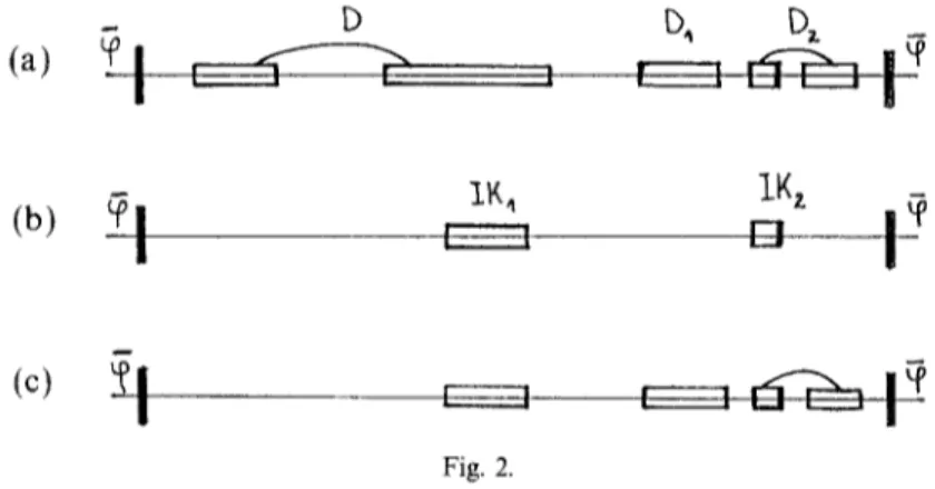
N o w we estimate the interaction between two contours K~ and Kj, the interaction between two interface contours IK~ and IKj, and the interaction between contour K~ and interface contour IKj.

Suppose supp Kl = [at, bl] and supp IKt = [a/, bt]. Let supp I K + = [bl, ai+ 1] and supp i K 7 = [-bi_ 1, ai]

where bo = p if there exists K e PB(~o'(x)) such that supp K = [ - o% p ] and bo = - o o otherwise; and am+l = q if there exists K ~ PB(~o'(x)) such that supp K = [q, oo ] and am + 1 = oo otherwise.

1. The contour K i e PB(q~'(x) ) interacts with the contour Kj ~ PB(q~'(x) )

through all pairs (x, y) such that (x, y ) e I n t ( K i , Kj) and f ' ( x , y ) r where

The value of the interaction is

f ' ( x , y) = U(x - y)(q/(x) qr

-- ~lKi(X) ~]Ki(Y) "~ ~!)i~r ~oi~(Y)

- Oxj(x) Oxj(Y) + (o~(x) (ok(y))

(42) 2. The interface contour

IKie PB(qr

interacts with the interface contour

IKjePB(~o'(x))

(let

aj>bi)

through all pairs (x, y) such that (x, y) ~ Int(IKi,

IKj)

and f"(x, y) ~ O, where

Int(IKi, IKj) = Int l(IKi, IKj) + Int2(IK;,

IKj)

+ Int3(IK~, IKj) + Int4(IK~,

IKj)

Intl(IKi, IKi) = [(x, y): x, y e Z1; x e supp

IK i and y ~ supp

IKj]

Int2(IK;,

IKy) =

[(x, y): x, y e Z1; x e supp

IK~ and y e supp

IK + ]

Int3(IKi, IKj)

= [(x, y): x, y ~ Z1; x ~ supp

IK 7

and y e supp IKj] Int4(IK~, IKj) = [(x, y): x, y e Z1; x e supp

IK 7

and y ~ supp

I K f ]

The value of the interaction is

f"(x, y) = f f ( x , y) = U ( x - y)(q/(x) q)'(y)

- Oix,(x) OlK,(Y) + FPi~(x) (pi(y)

- 0IN(x) O,~(Y) + qS{(x) ~;~(y))

(43)

if (x, y) e Intl(IK~,

IK;);

f"(x, y) =f;'(x, y) = U(x - y)(q)'(x) (p'(y)

- OiK~(x) OIK,(Y) + (Pi~(x) FP~(Y))

(44) if (x, y) e Int2(IK~, IKj);

r"~x y ) = ~ , , y ) =

U(x-y)(~o'(x)~o'(y)

-- O,Kj(x) OIKj(Y)) + ~bs qSJ(y)) (45) if

(x, y) e Int3(IKi, IKj);

and

f"(x, y ) = f'4'(x, y ) = U ( x - y)(q)'(x) qo'(y)

-1,i - l i ~92j

- ~o~ (x) ~o; ( y ) - ; (x) (o~,;(y))

if (x, y) s Int4(IKi,

IKj)

tion 3 ].

(46) [the configuration (bl~'i(x) is defined in Defini-

Absence of Phase Transitions in 1 D AF Models 589

3. The contour

K~ePB(~o'(x))

interacts with the interface contour

IKjePB(~o'(x))

through all pairs (x, y) such that (x, y ) e I n t ( K i ,

IKj)

and

f " ( x , y) ~ O, where

Int(Kg, IKj) = Intl(K~, IKj) + Int2(K~, IKj)

Intl(K~,

IKj)

= [(x, y): x, y e Zl; x e supp Ki and y e supp IKj] Int2(Ki, IKj) = [(x, y): x, y e Zl; x e supp K i and y E supp IK + ] if aj > b~, and

Int2(K/,

IKj) = [_(x, y): x, y e Zl; x e supp Ki and y e supp I K f ]

if ai > bj.

The value of the interaction is

f " ( x , y) = f'('(x, y) = U(x - y)(q~'(x) q)'(y)

- ~PI~(x) OKi(Y) + (Pi,,(x) (Pi~(Y)

- ~,,~(x) r

+ r

~ ( y ) )

if

(x, y) ~ Int'(Ki,

IKj),

and

f " ( x , y)=f~"(x,

y)

(47)

= U ( x - y)(~o'(x) q)'(y) - $K,(x) tPl~,(y) + ~ ( x ) (pi(y))

(48) if (x, y) e Int2(Ki, IKj).

By using the formulas (42)-(48) later we shall introduce and investigate the noninteracting contour model.

The following lemma will be extremely useful for the further calcula- tions.

I_emma 4. 1. Let us consider two contours (usual or interface), say K~ and Kj. Suppose supp K i = [a~, b~], supp Kj = [aj, bj], or supp Kj =

[aj, + ~ ] and the distance between supp Ki and supp Kj is

a j - b i =

Ri, j > 0 . Let

s u p p K ~ = s u p p l K i w s u p p 2 K ~

and

s u p p K j = s u p p ' K j w

supp 2 Kj (see the definition of the essential and regular parts of the support of a contour), and N = min(lsupp 1 Kil, Isupp 1 Kj[). Then

IG(Ki, Kj)t =

~.

If(x, Y)t <~ ClRi, f N ' - ~

(x, y) ~ I n t ( K i , / 0 )

(49)

Proof. Part A. Let us consider two intervals [a, b ] a n d I-c, or) such that b - a = N1, a n d c - b = R > O. Consider the following expression:

T h e n G(a, b, c) = ~ 5 U ( x - y) (50) x, y a Z l ; y 6 : [_a,b] a n d x ~ [ c , ~ ] G(a, b, c) <~ C 1 R o: 1 ~. N 1 C 1 = 30A I n fact, R+N1 G ( a , b , c ) = ~ U ( i ) ( i - R + I ) + ( N , + I ) i=R - ~ S I ~ - S 2 S 1 ~Stl = U ( R ) + U ( R + z ) ( z + 1) dz

U(j)

j = R + N I + I (51) ;~1 f ~ l

= U(R)+

U(R+z)(R+z)dz-

U(R+z)(R-1)dz

= U(R) + Ix - I2 (52)

By using the c o n d i t i o n U(x) ~ A x - t _ ~, 0 < e < 1, we have (R ~ ~ )

U(R) ~ A R - I - Ii ~ A ( 1 - - g ) - ~ ( ( R + N , ) ~ - ~ - ( R + 1 ) ( 1 - ~ ) ) ~ A N 1 1 - ~ R - ~ (53) I2 ~ Ag I(R - 1 )((R + 1 ) ~ - (R + N1 ) ~) ~ A N ~ - ~ R - ~(R - 1 )/R Therefore, I I - I 2 ~ A N 1 ~ R - ~ ( 1 - ( R - 1 ) / R ) ~ A N I - ~ R 1 ~ (54) Finally, f r o m (50)-(54) we get

81~81~ CIR-I-~ l-a;

' N~ C 1 = 3A (55) N o w note t h a t S2 = (N1 + 1 ) ~ U(j) <~ S'2 j=R+NI+I

;)

= ( U ~ + 1)

U(R+Ni+

11 + ( U l + 1)

U(z) az

= R + N I + I = (Ul + 1) U(R + Ul + 1 ) + I ~ (56)

Absence of Phase Transitions in 1 D AF M o d e l s 591

By using the condition U(x) ~ A x - 1 - ~, 0 < a < 1, we have (R ~ ~ )

(Ul + 1) U(R + N1 + 1 ) ~ A R - I - ~ ' N ~ ~ (57) I2 ~ Aa(N1 + 1)(R + Na + 1) -~ ~ A ~ R - ~ N ~ ~ (58) Finally, from (56)-(58) we get

S 2 ~ C a R ~Nll - ~; Ca = 3A Finally,

(51).

Part B.

(59) the inequalities (55) and (59) yield the required inequality

Let us consider two segments [a, b] and [c, oo) such that b - a = Ma and c - b = R > 0. Suppose that K is an arbitrary c o n t o u r with s u p p K = I-c, ~ ) ; Ola. b and 0~.b are two regular phases. Consider the

following expression:

Gr(a, b, c) = E 5U(x -- y)(O~,b(x) ~o(y) -- ~bza.b(X) ~p(y)) x, y~Zl;x~ [a,b] andy~ [c, oo)

(6o)

T h e n

Gr(a,b,c)<~C1R-1 ~; C l = 3 0 A n o (61)

First, note that there exists a n u m b e r p ' < n o such that Oa, b(X) = l

tpla, b(X + p). Therefore

U ( x -- y)(~lla, b(X) q ) ( y ) -- I//~,b(X ) q ) ( y ) )

< ( V ( y - x ) - U ( y - x + p) <. C o V ( x - y ) / ( x - y)

where Co = ~P' < ~no. T h e n

1/CoGr(a, b, c) <~ ~ U(x - y ) / ( x - y)

x,y~Zl;x~ [a,b] andya I-c, ~ ) R+NI = ~ ( i - - R + 1) U(i)/i+ ( M I + 1). U(j)~[ i--R j = R + M I + I

=s~+s~

F

s~ < U(R)/R + ( z + 1) U(R + ~)/(R + ~) d~

F

= U(R)/R + U(R + z) d~

f?

- ( R - 1) U ( R + z ) / ( R + z ) & = U(R)/R + I~ - I~ (62)

By employing the condition U ( x ) ~ A x ~ ~, 0 < ~ < 1 , we have ( R ~ ) U ( R ) / R ~ A R - 2 - I~ ~ A ~ - ~((R + 1 ) ~ - (R + M1) - ~) (63) I ~ A ( I + ~ ) I ( R - 1 ) ( ( R + I ) - I - ~ - ( R + M 1 ) ~-~) Therefore, Ir~ -- V 2 "~ A R 1 --~ (64)

Finally, from (62)-(64) we get

S~1<~ C I R 1 ~; C 1 = 3A (65)

Now note that

S~ -- (M1 + 1) L U ( j ) / j j = R + M I + I ~< (M1 + 1 ) U ( R + M1 + 1 )/(R + M1 + 1 )

;)

+ (M~ + 1 ) U(z)/z dz = R + M I + I = (M~ + 1) U ( R + M ~ + 1 ) / ( R + M 1 + 1 ) + I ~ (66) By using the condition U(x) ~ A x 1 ~ 0 < ~ < 1, we have (R --* ~ )

( M ~ + I ) U ( R + M I + I ) / ( R + M I + I ) < < A R 1 ~ (67) I ~ A ~ ( M I + I ) ( R + M I + I ) ~ ~<~AR - 1 - ~ (68) Finally, from (66)-(68) we get

S~2 <~ C 1 R - 1 - ~ ; C1 = 3 A (69)

Finally, the inequalities (65) and (69) lead to the required inequality (61).

We estimated the interaction between a finite contour and an infinite contour in Part A and the interaction between a finite regular phase and an infinite contour in Part B. Now we start directly to prove the statements of Lemma 4. We divide the proof of the inequality (49) into three cases.

Absence of Phase Transitions in 1 D AF Models 593

The interaction between K1 and K2 can be estimated as [see (42)]

a(gl,

g2) = 2

f'(x, y) <~

~

5U(x - y)

(x, y) ~ Int (Ki, Kj) (x, y) ~ Int (Ki, Kj)

Let supp K i = supp 1

K~w supp 2 K,, supp K j = supp ~

K;w supp 2 K:, and

N = min([supp I K~[, [supp 1 Kj[ ). The set of all pairs (x, y ) ~ Int(K,., Kj) such that x e s u p p l Kg and y ~ s u p p l K j we denote by E. Then

G ( K 1 , K 2 ) ~ 2 5 g ( x - y ) + ( x , y ) e E

Now note that

S~ ~ G(a, b, c) =

6 U ( x - y ) = S l

+ S 2

(x, y) ~ I n t ( ~ , ~ ) ; (x, y) ~ E

Y~

5 U ( x - y)

x , y ~ Z l ; y E [a,b] a n d x ~ [c, ac ]

where b - a = N and c - b = R. According to the inequality (51),

S I ~ C I R

~N 1 ~; C 1 = 3 0 A

In addition, because of the inequality (61) we may write

$2<~CIR-1-~;

Cl=30Ano

Hence in the first case the proof of the statement (49) is completed. 2. Suppose that we have one ordinary and one interface contour, say Ki and

IKj.

The interaction between Ki and K2 can be estimated as [see (47), (48)]:

G(K,, IKj) =

Y"

f " ( x , y)

(x, y) ~ Int(Ki, IKj)

=

~

ff'(x, y)+

~

f;"(x, y)

(x, y) ~ Intl(Ki, IKj) (x, y) ~ Int2(Ki, IKj)

=

y~

5 V ( x - y) +

Y~

J 2 ' ~ ' Y )

,~'~x

(X, y) E I n 0 (K/, IKd) (x, y) ~ Int2(Ki, IKj)

= S 1 --[- S 2 (70)

As in the first case, we have

SI<~C1R

~N 1-=; C 1 = 3 0 A

N o w note that the formulas (47) and (48) allow us to apply the inequality (61) and to get the following estimation:

Therefore in the second case the proof of the statement (49) is completed.

3. Suppose that we have two interface contours, say IKi and IKj.

The interactiopn between two interface contours IK1 and IK 2 can be estimated as [see (43)-(47)]

G(IK1,

IK2)=

~ f " ( x , y)

(x, y) ~ Int( IKi, IKj) 4 = E Z f " ( x , y) n = 1 (x, y ) e l n t n ( l K i , IKj) 3

5v(x- y)+

(x, y) ~ Intt(1Ki,IKj) = $1 + $2

As in the first case

f~(x, y)

n = 1 ( x , y ) E l n t n ( I K i , l K j )

Sa <~ C1R-~'N 1 ~; C 1 = 30A

Now note that the formulas (43)-(47) allow us to apply the inequality (61) and to get the following estimation:

S 2 ~ C 1 R 1-c~; Cl=90Ano

The p r o o f of L e m m a 4 is completed.

Now we shall prove seven auxiliary lemmas. Suppose that the bound- ary condition qS(x)=[~o(x), x ~ ( - o o , - V - 1 ] u [ V + l , oe)] is fixed. The set of all configurations 9(x), x ~ [ - V , V], we denote by q~(V). Let q)'(x) e ~(V), and an ordinary contour K and an interface contour IK

belong to PB(q/(x)).

Lernma 5. There exists a positive constant t, depending only on the Hamiltonian (1), such that the weight of an ordinary contour K satisfies the following inequality:

7(K) > t Isupp I KI where t is the constant defined in Lemma 1.

Proof. Lemma 5 is a consequence of formula (4) and Lemma 1. Indeed, let a contour K contain precontours PKi, i= 1 ... m. This implies that supp 1 K = 0 era= 1 supp PKi.

Absence of Phase Transitions in 1 D AF Models 595

The function of interaction G(PKI,... , PKm) is a decreasing function of the distance between precontours. Therefore

7(K) = ~ 7(PK) G(PK1 ... PKm) > 7(K)

i = 1

where the contour K7 is obtained by merging all neighboring precontours (thus [supp K[ = Isupp 1 K'[ = z,.ml [Z~'- 1 ~(PK)[ = [supp t K]).

But according to Lemma 1, 7(K)> t [supp/s Therefore, ~(K) > t [supp ~ K[

Lemma 5 is proved.

Let us consider an arbitrary configuration q~'(x) ~ q~(V). The boundary of the configuration qa'(x) includes a finite number of ordinary contours K~, i = 1,..., n, and a finite number of interface contours IKi, i = n + 1 ... n + m. Let K i = K~, i = 1 ... n, and K~= IK~, i = n + 1,..., n + m. The weights of the K~ (contours and interface contours) are defined by formulas (4) and (5).

Let K t be an arbitrary contour of the boundary B(q~'(x)),

[ s u p p m K t [ = N z ; Ko=q3(Ko), suppK0, where K o = ( - o o , - V - 1 ] w [- V + l, oo); the distance between supp K t and supp Ko is Rl.

I . e m m a 6. Suppose Nb > 6Cx/t ~/~ (Nb is a constant introduced in the definition of a contour). Then

n + m

7(K,)/6> IG(Kt)] = ~ [G(K,, Ks) ]

j = l ; j ~ l

ProoL Lemma 6 is a consequence of Lemmas 4 and according to Lemmas 4 and 5,

IG(Kt)] < C~ N b ~ N ~ ~ < tN~/6 < 7(Kt)/6 if N~ > 6C~/t. Lemma 6 is proved. (71) 5. In fact, k e m m a 7. Suppose R t > 6C~/t ~/~. Then 7(K,)/6 > ]G(Kz, K0)l

Proof. Lemma 7 is a consequence of Lemmas 4 according to Lemmas 4 and 5,

if R~ > 6C1/t.

and

]G(K,, Ko)] < C 1 R , =N ,l-c~ < t N , / 6 < y(K,)/6

(72) 5. In fact,

Lemma 7 is proved.

L e m m a 8. Suppose N t > 6C1/t 1/~. Then

7(K,)/6 > IG(K,, Ko)l (73)

Proof. Lemma 8 is a consequence of Lemmas 4 and 5. In fact, according to Lemmas 4 and 5,

IG(K~, Ko)l < C 1 R T " N ~ - ~ < tNJ6 < 7(K1)/6

if N~ >

6C1/t.

Lemma 8 is proved.

Suppose IK is an interface contour. Let us consider the configuration $~x such that the boundary of the configuration $IK includes only the con- tour IK (see Definition 3). Let the special ground states 9n0(x) and q~Z0(x ) be defined as in Definition 3. The set of all configurations ~0'(x)e q~ such

that PB(r contains the only interface contour and the same special

ground states ~oln0(x) and (p]0(x) we denote by q~1,2.

L e m m a 9. Let the configurations q~(x), r I~ 1'2 contain unique

interface contours IK and IK', respectively, and two regular phases $ l ( x ) and $2(x). Moreover, let the restriction of the configuration ~o'(x) on supp IK coincide with (p(supp IK) and Isupp IK'] - Isupp KI > Nb.

There exists a positive constant t depending on the Hamiltonian (1) only, such that the weight of any interface contour IK satisfies the following inequality:

7(IK') - 7(IK) > t(]supp IK'I - Isupp KI - Nb)

ProoL Let the configurations cp and (p' be obtained, respectively, from the configurations q~(x) and (p'(x) by substitution of $2(x) by Sa(x). In other words, the configurations ~o and (p' are obtained by shifting of the regular phase $2(x) for some p < n o. The configurations q)(x) and ~o' contain the usual contours K and IK. Then

H(cp(x))-H(go)<<. ~ ( U ( x ) - U ( x + p ) ) x x E Z I ; x > 0 <<. ~ 2Ax(x ~ - ( x + p) ~1 xEZI;x~- 0 2A~px ~ < const ~< x a Z l ; ~ > O

Absence of Phase Transitions in 1D AF Models 597

and

H(~o'(x))-H(~o')<<.

~

(U(x)- U(x + p))x

x ~ Z l ; x > 0 <~ ~ 2 A x ( x ~ - ( x + p ) - ~ ) xEZ1;x>O <~ ~ 2 A ~ p x - ~ < const xEZI;x>O Therefore, y ( I K ' ) - ~(K) = H(ep'(x)) -- H ( $ l ( x ) ) - (H(~o(x)) -- H ( $ l ( x ) ) ) = H(q~'(x)) -- n ( ~ p ( x ) ) > H((p') - n(~o) - const Now note that according to Lemma 8

H(cp'(x)) - n ( ( p ( x ) ) = y ( K ' ) - 7(K) > t(isupp IK'[ - [supp K[ - Xb) Lemma 9 is proved.

L e m m a 10. There exists a configuration ~0min(X ) ~ 1 2 051,2 such that

/-/(~01,2(x)) - m ( ~ o ( x ) ) / > 0

for each configuration q~(x)~ ~1,2. Let I K ~ i 2 be a unique contour of the configuration ~0mi n. Then Isupp ~ 2 IKmi n] 1,2 < 3d0no + Nb.

P r o o f . Lemma 10 is a consequence of Lemma 9.

Indeed, let us consider the configuration q~(x)E ~1,2 with the unique interface contour K such that ]supp IK[ <3dono [-the existence of the configuration q~(x) is obvious]. Then according to Lemma 9

[supp _[Kmin[ 1,2 _{< [supp IKI + Nb < 3dono + Nb}

I . e m m a 11. Suppose ~o(x), q ) ' ( x ) ~ ( V ) and the restriction of q~(x) on some segment [a, b ] ~ [ - V + Nb, V - -

Nb]

coincides with a special ground state q~0(x). The configuration ~0'(x) is some perturbation of q~(x) on the segment [a, b]. The set PB(q)'(x); [a, b ] ) is the set of all contours (usual and interface) K ~ P B ( ~ o ' ( x ) ) and s u p p K i ~ [a, b]. Suppose that PB(q~O'(x); [ a , b ] ) = U ' ; = l K i 9 Then there exists a positive constant t depending on the Hamiltonian (1) only, such that

•

~,(Ki) > t ~ Isupp I Kil

Proof. The proof coincides with the proof of Lemma 5. Now we are ready to prove the following result.

L e m m a 12. Suppose that the boundary conditions q3(x)= [~o(x), x e ( - o% - V - 1 ] u [- V + 1, oo )] are fixed and Nb > 6C1/t 1/~. The set of all configurations q~(x), x 9 [ - V, V], we denote by 4(V). Let q~min(X) 9 qS(K) be a configuration with the minimal energy

g((Pmin(X)) = lim H(qo(x)) (74)

cp(x) E ~ ( K )

Then the configuration ~0min(X) has the following structure:

The restriction of the configuration q~min(X) on the set [ - V + N b ,

V--Nb] contains at most no--1 contours; moreover, all of them are interface contours IKi, i = 1 ... m, where m < n o - 1 and I s u p p l K i l < 3d0n0 + Nb.

Proof. Let the boundary of the configuration ~0'(x) include a finite number of ordinary contours Ki, i = 1 ... n, and a finite number of interface contours IKi, i = n + 1,..., n +m. The set of all contours of the boundary conditions qS(x) will be denoted by Ko.

The following equation is a direct consequence of the formulas (4) and (5):

n + m n + m

H(~p'(x))--H(P,o(X))= ~ 7(Ki)+ ~ G(Ko, K1 ... Kn+m) (75)

i = 1 i , j = O ; i < j

where ~on0(x ) coincides with a special ground state ~bl~(x) (see Definition 3) defined for the first from the left contour (ordinary or interface) Ki,

i= 1,..., n + m, and the multiplier G(Ko, K1,..., Kn+,,) corresponds to the interaction between contours (ordinary and interface) and with the boundary conditions,

t / + m

a(Ko, K~,..., Kn+m)=

2

G(K, Kj) (76)

i , j = 0 ; i < j

Let K~, i= i~ ... ip, be an arbitrary ordinary contour of the boundary B. Then automatically a distance Ri between supp K~ and supp g is greater than Nb. Then according to Lemma 6

H((p'(x)) - H ( ( p i ( x ) ) = ~ ( K i ) - [G(K31 >/0

where the configuration ~pi(x) is obtained from the configuration q/(x) by deleting of contour Ki.

Absence of Phase Transitions in 1 D AF Models 599

By continuing this procedure we get

H(~o'(x) ) - H ( e i , , .,ip(x) ) > 0

where the configuration (pil'"ip(x) is obtained from the configuration q)'(x) by deleting of contours Kil,..., Kip.

Let [Kz, i=ip+l ... ip+q] be a set of all interface contours of the boundary B, such that the distance Ri between supp Ki and supp k is greater than Nb.

According to Lemma 11, upon deleting all interface contours except at most n o - 1 (we have at most no distinct regular phases which correspond to no distinct special ground states), we can obtain the configuration

(])del __ ~oil,...,ip,ip+ l,...,ip+q,g(X )

such that

O((19'(x)) - O ( ( p d e l ) ( x ) > 0

Further, let K 1 and K2 be a contours with [supp Ki[ >Nb, i= 1, 2,

such that s u p p K l = [ a l , b l ] u [ b 1 + 1 , c l ] and s u p p K 2 = [ c 2 , a 2 - 1 ]

[-a2, b 2 ] , where bl = - - V + N b and a2--- V - - N O. Then, according to Lemma 8,

H ( ( p del) - n ( ( p del'l ) > 0 ₍₇₇₎

where the configuration @del, 1 is obtained from the configuration @del

by deleting of contours K'I = (~odel([bl + 1, cl], [bl + 1, Cl]) and K; =

( ( p d e l ( [ c 2 , a 2 -- l ] , [-c2, a 2 - - l l ) .

The inequality (77) shows that a configuration with the minimal energy contains at most n 0 - 1 interface contours in the interval

[ - V+ Nb, V - Nb]. Let supp IKi be an interface contour of the configura- tion CPmin(X ). According to Lemmas 10 and 6,

[supp IKil < 3don o + Nb

Therefore, there exists a configuration (~9 del'2 such that

H(q0del, 1) __ H ( ~ d e l , 2 ) > 0 ₍₇₈₎

where the configuration ~0 del'2 is obtained from the configuration (19 del'l by chopping of large interface contours (contour IKi is said to be large if

[supp Igi[ > 3dono + Nb). Lemma 12 is proved.

By using Lemma 12 we shall give a full description of the set of all ground states.

We know that each special ground state is a ground state (see Remark 2).

T h e o r e m 4. Let the value of the external field # of the model (1) belong to the interval (#~-, #+ ) for some number ic = q/p = 1~no. Suppose that r is a ground state of the model (1). Then the configuration (p'(x) contains at most n o - 1 interface contours IKg such that IsupplK;[ < 3d0n0 + Nb < const.

Proof. Theorem 4 is a direct consequence of Lemma 12. Indeed, let q)'(x) be a ground state of the model (1).

Let us consider an arbitrary segment [ - V , V], and a boundary condition ( o ( x ) = [ ~ o ' ( x ) , x ~ ( - o o , - V - 1 ] u [ V + l , oo)]. The set of all configurations q)(x), x e [ - V , V], we denote by 45(V). Suppose a configuration q3min(X)e 45(V) is a configuration with the minimal energy [see (75)].

According to the definition of the ground state, (1) for each

xE[--V+ Nb, V-Nb]

(Pmin(X) ~--

q)t(X)

and the configuration r according to Lemma 12 has the required form in the segment [ - V + Nb, V - N b ] . Note that V can be chosen arbitrarily large. The proof of Theorem 4 is completed.

Theorem 4 shows that each ground state is a special ground state or a combination of several special ground states.

3. G I B B S S T A T E S . T H E D E N S I T Y K IS 1 I n o

In this section we prove the uniqueness of the Gibbs states for special values of the external field (when the density of the special ground state is 1/no). The general case will be considered in Section 4.

Suppose that the value of the external field # of the model (1) belongs to the interval (#~-,/~+ ) for some number ~c = q/p = 1~no, and the boundary conditions O(x) = [q~(x), x ~ ( - oo, - V - 1 ] u [ V + 1, oo)] are fixed.

Let ~0(x)E 45(V) be an arbitrary configuration; the boundary of the (p(x) includes a finite number of usual contours Ki, i = 1,..., n, and a finite number of interface contours IKi, i = n + 1 ... n + m. Let K~ = K~, i = 1 ... n, and K~ = IK~, i = n + 1 ... n + m. The set of all contours of the boundary conditions O(x) will be denoted by Ko.

Absence of Phase Transitions in 1 D AF Models 601

The statistical weights of contours and interface contours are

w(Ki)

= exp( -/~7(K~)) Let

H( ~o(x) l (o(x) ) = -~t

y~

~(x)

x E Z l , x e [ - v , v ]

+

E

x, y c Z l , x > y;x, y E [-- V, V]

+

E

x , y ~ Z l , x > y ; x e [ - - V , V ] ; y r

+

E

x, y e Z l , x > y ; x r [ - V, V ] , y e [-- V, V]

U(x- y)~(x)~(y)

U(x- y) ~(x)~(y)

U(x- y) ~(x)~(y)

(79)

The following equation is a direct consequence of the formulas (4), (5), and (79):

r/ -t- m

exp{

-~H(~o(x) l(o(x))} = I~ w(Ki)

exp{

-[3G(Ko, K1 ...

K,+m)} (80)

i = 1

where the multiplier

G(K o, K1,..., Kn+m)

corresponds to the interaction

between contours [-usual and interface; see (42)-(48)] and with the boundary conditions q3(x): n W m

G(Ko, K1,...,

K , + m ) = ~

G(Ki, Kj)

i , j = O ; i < j

= ~

~

f(x, y)

(81) i , j ; i < j ( x , y ) ~ I n t ( K i , K j )

For simplicity, Ki, i = 1 ... n + m, will be denoted by Ki, i e I, where the statistical weights are defined by the formulas (79), (4), and (5). Thus, the formula (80) has the form

exp{-flH(~p(x)lCo(x))} = I~ w(K~)exp{-flG(Ko, K1

... Kn+m) } (82)

i e I

The set of all pairs (x, y) in the double sum (81) will be denoted by G. Write (82) as follows: exp{-/~H(cp(x)lO(x))} = H

w(K~) I~

{1 + e x p ( - / ~ f ( x , y ) - 1)} (83) i ~ l ( x , y ) ~ G From (83) we get

exp{-BH(~o(x)l(o(x))}= ~

~I w(K~)

~I

g(x, y)

(84) G ' c G i ~ l ( x , y ) ~ G ' ; f ( x , y ) ~ O 822/72/3-4-13

where the summation is taken over all subsets G' (including the empty set) of the set G, and

g(x, y ) = e x p ( - f l f ( x , y ) ) - 1.

Consider an arbitrary term of the sum (84), which corresponds to the subset

G ' c G .

Let the bond

(x, y)eG'.

Below, contours and interface contours will be called contours. Consider the set K of all contours such that for each contour K c K, the set supp Kc~ (x u y) contains one point. We call any two contours from K connected. The set of contours K' is called G' connected if for any two contours Kp and

Kq there exists a collec-

tion ( K 1 ----Kp,

K2,..., K,,

= Kq) such that any two contours Ke and Ke+ 1,

i = 1,..., n - 1, are connected by some bond (x, y) ~ G'.

D e f i n i t i o n 4. The pair D = [(Ki, i = 1,..., s); G'], where G' is some set of bonds, is called a cluster provided there exists a configuration q~(x) such that

K~ePB(9(x)), i= 1,..., s; G ' c G;

and the set (K~, i = 1 ... s) is G' connected. The statistical weight of a cluster D is defined by the formula

w(D) = (I w(Ki)

l~

g(x, y)

(85)

i = l ( x , y ) ~ G '

Two clusters DI and D2 are called compatible provided any two contours K~ and K2 belonging to D1 and D2, respectively, are compatible and not connected. A set of clusters is called compatible provided any two clusters of it are compatible.

If D =

[(Ki,

i = 1 ... s); G'], then we say that

K~eD, i= 1,..., s.

I . e m m a 13. Let boundary conditions ~(x) = [q~(x), x ~ (- ~ , - V - 1 ] u [ V + 1, oe)] be fixed.

If [D1 ... Om] is a compatible set of clusters and u i m l s u p p D i c

[ - V , V], then there exists a configuration ~o(x) which contains this set of clusters. F o r each configuration ~o(x) we have

exp{-flH(~0(x)l qS(x))} = ~ 1~

w(Di)

G ' = G

where the clusters Dr are completely determined by the set G'. The partition function is

-~(~(x)) = ~ w(D1)..,

w(Dm)

where the summation is taken over all nonordered compatible collections of clusters.

Absence of Phase Transitions in 1 D AF Models 603

i - - = = I | ~ d i

(a) (b)

Fig. 1.

Lemma 13 shows that we come to noninteracting clusters from inter- acting contours. Figure la shows contours K~ and

IK2

of a configuration q~(x) and Fig. lb shows a cluster (one of many) corresponding to these contours.

k e m m a 14. Let D = [(Ki, i = 1 ... s); G'] be an arbitrary cluster. Let supp 1D = Zs= 1 supp ~ Ki and tl --

5t/6,

where t is the constant defined in Lemma 5. Then

w(D)

< exp(--fltl Isupp I DI)

Proof.

This

w(D) =

lemma follows from Lemmas 5 and 6. Indeed,

(I w(I,:,) 1-I g(x, y)

i = 1 (x,y)~G'

< ~ e x p ( - f l t [supp 1

Ki] )

i = 1

~< 11I e x p ( - f l t Isupp 1 K/I)

i = 1

<~exp{--fl L tlsupplKi,+

i = 1

< exp( - 5 f i t Isupp 1 DI/6)

fI g(x, y)

(x,y)~G' [ I exp(tflf(x, y)[) (x,y)~G'

B If(x,

yl]} ( x , y ) e G ' Lemma 14 is proved.

L e m m a 15. Suppose that the value of the external field /~ of the model (1) belongs to the interval (/~-, #+ ) for some number • =

q/p = 1~no,

and boundary conditions ~(x) = [~0(x), x e ( - o% - V - 1 ] w [ V + 1, Go)] are fixed.

In the proof of Lemma 12 we have defined a configuration ~0 de~'2 for each configuration ~o(x)E ~b(V). Let us consider the set of all configurations (pae~'2(x). According to Lemma 12 (a boundary of each configuration