Geometric-zero truncated poisson distribution: properties and applications

Journal of Science

http://dergipark.gov.tr/gujs

Geometric-Zero Truncated Poisson Distribution: Properties and Applications

Yunus AKDOGAN1,* , Coskun KUS1 , Hamid BIDRAM2 , Ismail KINACI3

1 _{Selcuk University, Department of Statistics, Konya, Turkey} 2 _{University of Isfahan, Department of Statistics, Isfahan, Iran} 3 _{Selcuk University, Department of Actuary, Konya, Turkey}

Article Info Abstract

In this paper, a new discrete distribution is introduced by compounding the geometric distribution with a zero truncated Poisson distribution, named geometric-zero truncated Poisson (GZTP) distribution. Some basic properties of the new distribution, such as the hazard rate function, moments, mode, median, etc., are studied. We show mathematically and numerically that the hazard rate function is increasing. The model parameters are estimated by the moment, least squared error and maximum likelihood methods. A simulation study is performed to compare the performance of the different estimators in terms of bias and mean squared error. An application of the new model is also illustrated using the three real data sets.

Received: 21/10/2018 Accepted: 16/03/2019 Keywords Compounding Estimation Geometric distribution Zero truncated Poisson distribution

1. INTRODUCTION

In recent years, several new continuous distributions have been introduced by compounding an absolutely continuous distribution with a discrete distribution in the literature. For example, exponential-geometric (Adamidis and Loukas [1]), Weibull-geometric (Barreto-Souza et al.[2]), Weibull-Poisson (Hemmati et al. [3]; Lu and Shi [4]), exponential-Poisson (Kuş [5]), exponential-logarithmic (Tahmasbi and Rezaei [6]) are some remarkable distributions in this connection. Unlike continuous compound distributions, which are created by compounding an absolutely continuous distribution with a discrete one, discrete compound distributions, i.e., compounding two discrete distributions, have not received much attention in the literature, especially in reliability context and statistical modelling.

There exist some complex systems in reliability having components with discrete distributions (see, e.g., Kemp [7] and Noughabi et al. [8]). Now, if the components of a system are themselves random variables with a discrete distribution, then compounding these two discrete distributions can be applied to the lifetime of parallel or series systems. Indeed, the distribution of maximum (minimum) of N components can be obtained by compounding method and has many applications in parallel (series) systems in reliability. Some studies in these subjects can be addressed as uniform-geometric distribution of Akdoğan et al. [9] and uniform-Poisson distribution of Gomez-Deniz [10]. In this paper, we are going to introduce a new discrete distribution by compounding a geometric distribution with a zero-truncated Poisson distribution. The new two-parameter discrete distribution has an increasing hazard rate function, which can be used in modeling discrete real data. This property is proved mathematically under a theorem.

The paper is organized as follows. Section 2 introduces the proposed discrete distribution with its properties, such as probability mass function (pmf), cumulative distribution function (cdf), hazard rate *Corresponding author, e-mail:yakdogan@selcuk.edu.tr

and quantile functions as well as median and mode. Section 3 involves moments. The statistical inference is discussed in Section 4. A simulation study is performed in Section 5. Finally, an application of the new discrete model is illustrated in Section 6. Concluding remarks are given in Section 7.

2. PROPOSED DISCRETE DISTRIBUTION AND ITS PROPERTIES 2.1. Letters Pmf and Cdf of the Proposed Distribution

Let

Y Y

₁

,

₂

,



,

Y

_N be

N

independent identically distributed (iid) random variables having a geometric

distribution with the pmf: 1

( ) y ; 1, 2, , (0 1 1),

P Y;y ;pq - y;  < ; - <q p

and

N

be a zero-truncated Poisson random variable, independent of

Y

, with the pmf:

( ) ; 1, 2, ( 0). !(1 ) n e P N n n n e l l l l -; ; ; > -  (1) Now, let us define a random variable as

X

;

max

(

Y Y

1

,

2

,



,

Y

N

)

. Then, its corresponding pmf is

obtained by

(

)

(

)

1 1 1 1 1 1 ( ) ( | ) ( ) (1 ) (1 ) !(1 ) (1 ) _{( (1 ))} 1 ! ! x n n x n x n n n x _{x n} n n P P X x P X x N n P N n e q q n e q e q e n n l l l l l l _l ¥ ; -¥ -; - ¥ ¥ -; ; ; ; ; ; ; ; ; - -æ _{- ö÷} ç _{- ÷} ç _÷ ; ç_ç - _÷÷ - ç_{çè ÷÷ø}

å

å

å

å

(

)

1 1 1 ; 1, 2, 0; , x x q q x otherwise o o o -ìï _{- ;} ïï ; í ïïïî  (2)

where

o

;

e

-l

Î

(0,1)

. The cdf of

X

is obtained by

(

)

1 1 ( ) ( ) ( | ) ( ) 1 !(1 ) 1 ; 1, 2, , 1 x x X n n n x n q q F x P X x P X x N n P N n e q n e e e e x l l l l l l o o o ¥ ; -¥ -; - -; £ ; £ ; ; ; -; -; ;

-å

å



whose final form is given by

( )

1

0;

0

;

1, 2,

x q

x

F x

x

o o o

-ì

£

ïï

; í

_ï

;

ïî



(3)

distribution and will be denoted by X ~GZTP q

( )

,o . The random variable X is potentially useful in

various fields, especially in parallel systems considering discrete distribution for their components (see, e.g., Nakagawa and Zhao [11]).

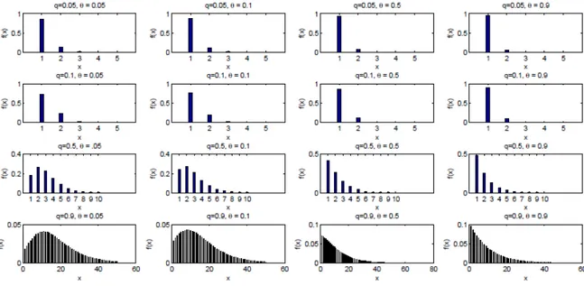
Figure 1 shows the pmfs of the GZTP q

( )

,o distribution for some parameter values of q and .o As we see from the graphs, for fixed values of ,q the pmf of the GZTP q

( )

,o distribution varies from increasing-decreasing to increasing-decreasing, when the parameter

o

increases.

Figure 1. The pmfs of GZTP q( , )o distribution for different values of q and o

Theorem 2.1. The pmf of GZTP q

( )

,o distribution is log-concave for any admissible value of q and .o Proof. We should show that P_x2³P P_{x-1 x+1} Keilson and Gerber [12]. Using pmf given in Eq. (3) we write

(

1

) (

2 1 2

)(

1

)

. x x x x x x q q q q q q o o - o - o - o + o - ³ -

-Now, consider the function

(

1

) (

2 1 2

)(

1

)

( ; , ) qx qx qx qx qx qx

g x q o ; o -o - - o - -o - o + -o . Then, one can show that ( ; , )

g x qo is decreasing for all xÎR+. In addition, it is clear that limx®¥g x q( ; , )o ; Therefore, 0. ( ; , )

g x qo is a non-negative function and then the proof is complete.

Corollary(Unimodal):

The pmf of GZTP q

( )

,o distribution is unimodal and its mode is

( )

(

)

( )

(

)

[ ] [ ]

{

}

( )

[ ]

(

[ ]

)

; 1 mod( ) 1; 1 , 1 ; 1 , m f m f m X m f m f m m m f m f m ì _{ê ú ê ú ê ú} ï > + ï ë û ë û ë û ïïï ê ú ê ú ê ú ;í _{ë û}+ _{ë û} < _{ë û}+ ïï ï _{+ ; +} ïïî

Proof. The unimodality of GZTP q

( )

,o distribution is achieved by the fact that log-concave pmfs are strongly unimodal and thus unimodal. (see, e.g., Keilson and Gerber [12]) To obtain mod(X), let us consider the pmf given in (pmf) be a continuous function in

x

.

Then, it is easy to see that the maximum

of the pmf happens at the point

(

log( )

)

( )

(1 ) log log _q q / log

m; _{- o} q .

2.2.

Hazard Rate Function

Let X~GZTP q( , ).o Then, the hazard rate function of X is given by

( )

(

)

(

)

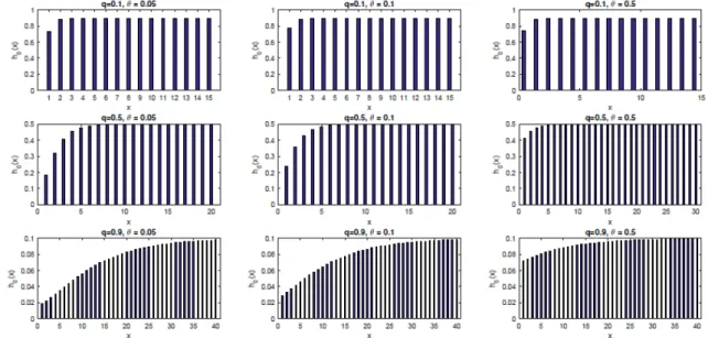
1 1 0 | ( ) ; 1, 2, 1 x x x q q q h x P X x x P X x P X x x o o o -; ; ; ; ³ -; ; - 

Theorem 2.2. The hazard rate function of GZTP q( , )o distribution is increasing for any value of q and o. Proof. It is obvious that log-concave pmfs have an increasing hazard rate function (see, e.g., Keilson and Gerber [12]). Thus, using Theorem 2.1, the hazard rate function is increasing for any value of q and .o The plots of hazard rate function are given in Figure 2. As we see from the graph, the hazard rate function of GZTP q( , )o is increasing for all values of q and o parameters.

Figure 2. The hazard rate functions of GZTP q( , )o for different values of q and o

2.4. Quantile Function

The quantile function of the GZTP q

( )

,o distribution, say Q u

( )

, is obtained by F Q u

(

( )

)

;u. Then, using

( ) . 1 Q u q u o o o -; - (4) Inverting Eq.(4), one obtains

( )

(

)

( )

1 log 1 . log u u Q u q o- _{- +} ;

From the non-decreasing property of Q u

( )

, the z th quantile

( )

x_z , of GZTP q

( )

,o distribution is given by

(

)

( )

( )

( )

(

)

( )

(

)

( )

( )

( )

1 1 1 log 1 1 ; log log 1 log 1 , 1 ; , log log x z u u Q z Q z q u u u u Q z Q z q q o o o ; -- -ì ê ú ï _{- +} ï _{ê ú} ï ₊ ê ú_¹ ï ê ú _{ë û} ï _{ê ú} ï _{ë û} ïïí ïæê _{- +} ú ê _{- +} ú ù ïç_{ê ú ê ú ú} ïç ₊ ê ú_; ïçê ú ê ú ú ë û ïç ïçê_çè ú ê ú ú ï ë û ë û û ïî

where xê ú_{ë û denotes the integer part of x . That is}

x

_z satisfies F x

( )

-_z £ £p F x

( )

_z , where F is the cdf of

( )

,

GZTP qo distribution given in Eq.(3). In a special case, the median of GZTP q

( )

,o distribution is also given by

(

)

( )

( )

( )

(

)

( )

(

)

( )

( )

( )

1 0.5 1 1 log 0.5 0.5 1 ; 0.5 0.5 log log 0.5 0.5 log 0.5 0.5 , 1 ; 0.5 0.5 . log log x Q Q q Q Q q q o o o ; -- -ì ê ú ï ₊ ï _{ê ú} ï ₊ ê ú_¹ ï ê ú _{ë û} ï _{ê ú} ï _{ë û} ïïí ïæê ₊ ú ê ₊ ú ù ïçê ú ê ú ú ïç ₊ ê ú_; ïçê ú ê ú ú _{ë û} ïç ïçê_çè ú ê ú ú ï ë û ë û û ïî 3. MOMENTS

3.1. Approximate and Exact Bounds of the Moments

Let X~GZTP q

( )

,o . Then the expected value is calculated by

( )

(

1

)

1 1 . 1 x x q q x E X x o o o -¥ ; ; --

å

(5) It is clear that E X( ) can not be calculated easily using the above equation. Therefore, we attempt to discuss an approximate value for E X

( )

here. A method for estimating the sum of a positive series, whose

convergence has been guaranteed, is the ratio test method. Let

1 n n S a ¥ ; ; å and 1 n n k k S a ; ; å be the n th partial sum. The ratio test method is given in the following lemma.

Lemma 1. (The ratio test; Braden [13]). Suppose { }an is a positive decreasing sequence such that

1 lim an 1. n an L + ®¥ ; < If 1 n a an + decreases to

L

, then

1 1 _. 1 1 n n n n n n a a a L S a S S L + + æ _ö÷ ç + ç_{çè -} ÷_÷ø< < +

Now, we discuss the expected value of GZTP q

( )

,o distribution in the following:

( )

(

1

)

1 1 1 1 1 1 1 1 , 1 x x q q x c x x x x c c x y c x y E X x a a a a o o o o o -¥ ; ¥ ; ; + ¥ + ; ; ; -å + å ; -å + å ;

-å

where ax x

(

oqx oqx1

)

-; - and c; ëêarg max

( )

ax úû. From Theorem 2.1, it is clear that a x is unimodal.

Furthermore

a

x is decreasing in

x

for x³c. By using ratio test method, one can obtain

( )

1 1 1 1 ₁ 1 1 1 n c an c an c n c n c _a q x n c x q _x x a a a E X o o + + + + + + + + - + å_; - + å_; £ £ - - ,

since { ;an n³ c} is positive decreasing sequence,

1 lim n c 1 n c a n a q + + + ®¥ ; < and n_nc_c1 a a + + + decreases to q. The

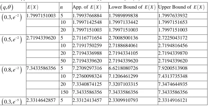
other moments can be obtained similarly. Table 1 contain first moment of GZTP q

( )

,o distribution for some parameter values. The true values of moments are provided by Maple software. Some approximations of moments are also presented for 5

e

o_; - _{and q;0.5 in Figure 3. From Tables 1-4, all} approximations are good enough n³150 for selected cases.

Table 1. Approximate value, lower bound and upper bound of E X

( )

( )

q

,

q

E X

( )

n

App. of E X

( )

Lower Bound of E X

( )

Upper Bound of E X

( )

(

2

)

0.3, e− 1.7997151003 5 1.7993766884 1.7989899838 1.7997633932 10 1.7997142548 1.7997133442 1.7997151653 20 1.7997151003 1.7997151003 1.7997151003

(

2

)

0.5, e− 2.7194339620 5 2.7116771654 2.7008500136 2.7225043172 10 2.7191750259 2.7188684061 2.7194816456 20 2.7194336988 2.7194334105 2.7194339870 50 2.7194339620 2.7194339620 2.7194339620

(

2

)

0.8, e− 7.3433586356 5 7.2709297316 6.6218080726 7.9200513908 10 7.2760098324 7.1206461299 7.4313735348 20 7.3340874125 7.3207103315 7.3474644935 150 7.3433586356 7.3433586356 7.3433586356

(

5

)

0.3, e− 2.3314642857 5 2.3312413457 2.3309910793 2.3314916121

10 2.3314637320 2.3314631392 2.3314643248 20 2.3314642857 2.3314642857 2.3314642857

(

5

)

0.5, e− 3.6795124171 5 3.6708662414 3.6590567668 3.6826757160 10 3.6792286275 3.6788966754 3.6795605796 20 3.6795121301 3.6795118170 3.6795124432 50 3.6795124171 3.6795124171 3.6795124171

(

5

)

0.8, e− 10.3715943115 5 10.2727957683 9.5103299111 11.0352616212 10 10.2921570783 10.1152364277 10.4690777314 20 10.3610415078 10.3462252766 10.3758577390 150 10.3715943115 10.3715943115 10.3715943115

Figure 3. Some approximate moments of GZTP q( , )o for q;0.5 and o ;exp( 5)

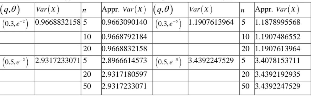
-3.2. Approximate and Exact Variance, Skewness, and Kurtosis

In this section, approximate and exact variance, skewness and kurtosis of GZTP q( , )o are given in

Tables 2-4.

Table 2. Exact and approximate variance for some parameter values of q and o

( )

q

,

q

Var X

( )

n Appr. Var X

( )

( )

q

,

q

Var X

( )

n _Appr. Var X

( )

(

_{0.3, e}-2

)

0.9668832158 5 0.9663090140

(

)

5 0.3, e- 1.1907613964 5 1.1878995568 10 0.9668792184 10 1.1907486552 20 0.9668832158 20 1.1907613964

(

_{0.5, e}-2

)

2.9317233071 5 2.8966614573

(

)

5 0.5, e 3.4392247529 5 3.4078153711 20 2.9317180597 20 3.4392192935 50 2.9317233071 50 3.4392247529

(

_{0.8, e}-2

)

28.2784602533 5 27.9418642698

(

)

5 0.8, e 32.5653946091 5 33.2237469999 20 28.1456910482 20 32.2997608568 50 28.2779548653 50 32.5644642142 150 28.2784602533 150 32.5653946091

Table 3. Exact and approximate Skewness for some parameter values of q and o

( )

q

,

q

Skewness X

( )

n _Appr.Skewness X( )

( )

q

,

q

Skewness X( ) n _Appr. Skewness X( )

(

2

)

0.3, e 1.5439885033 5 1.5293884914

(

_{0.3, e}-5

)

_{1.0913310183 5 1.0974467318} 10 1.5438744811 10 1.0913286139 20 1.5439885033 20 1.0913310183

(

_{0.5, e}-2

)

1.4760392637 5 1.4620813735

(

)

5 0.5, e 1.1516492654 5 1.1686130051 20 1.4760226997 20 1.1516370129 50 1.4760392637 50 1.1516492654

(

_{0.8, e}-2

)

_{1.4565690343 5 1.6365220116}

(

_{0.8, e}-5

)

_{1.1788315851 5 1.3763783197} 20 1.4392972052 20 1.1750124067 50 1.4564145782 50 1.1786652455 150 1.4565690343 150 1.1788315851

Table 4. Exact and approximate kurtosis for some parameter values of q and o

( )

q

,

q

Kurtosis X

( )

n _Appr. Kurtosis X( )

( )

q

,

q

Kurtosis X( ) n Appr. Kurtosis X( )

(

2

)

0.3, e 6.3909103067 5 6.4108993095

(

_{0.3, e}-5

)

_{5.1377052475 5 4.9970349940} 10 6.3908145204 10 5.1365329801 20 6.3909103066 20 5.1377052475

(

_{0.5, e}-2

)

6.3265775593 5 6.2994312225

(

)

5 0.5, e 5.3682140159 5 5.0740361546 20 6.3265408209 20 5.3680842138 50 6.3265775593 50 5.3682140159

(

2

)

0.8, e- 6.3183347918 5 6.2224533983

(

0.8, e-5

)

5.4654383959 5 4.8882486478 20 6.2211167752 20 5.3577364298 50 6.3173067981 50 5.4644336039 150 6.3183347918 150 5.4654383959

From Tables 3 and 4, it seems that GZTP q( , )o is rightly-skewed and leptokurtic.

4. PARAMETER ESTIMATION

4.1. Estimation by the Maximum Likelihood Method

log-likelihood functions based on the complete random sample are

(

1

)

1 1 ( , ) 1 xi xi n q q i L qo o o o -; ;

-Õ

and

( )

(

1

)

1 , log(1 ) log xi xi , n q q i q o n o o o -; ; - - +

å

-

(6)

respectively. Thus, the score equations are obtained by

( ) 1 1 1 2 1 , log ( 1) log 0 xi xi i i xi xi x x q q n i i q q i q x q x q q o o o o o o o -- -; æ ö ¶ _; ç_ç - - ÷_÷÷; ç _÷ ç ¶

å

çè - ÷ø 

(7)

( )

1 1 1 1 1 1 , 0. 1 xi xi i i xi xi x q x q n q q i q o n q o q o o o o o -- -; ¶ -; + ; ¶ -

å

-

(8)

The maximum likelihood estimation (MLE) of the parameters, i.e., qˆ and oˆ can be achieved by solving Eqs (7) and (8), using Newton-Raphson procedure. An approximate Fisher information matrix can be obtained by ( ) ( ) ( ) ( ) 2 2 2 2 2 2 , , ˆ ˆ ˆ ˆ ( , ) ( , ) , , ˆ ˆ ˆ ˆ ( , ) ( , ) | | ˆ ˆ ( , ) , | | q q q q q q q q q q q I q o o o o o o o o o o o o ¶ ¶ ¶ ¶ ¶ ¶ ¶ ¶ ¶ _¶ é_{- -} ù ê ú ê ú » ê_{- -} ú ê ú ë û    

(9)

whose entries are the estimated second order derivatives of Eq. (6). It can be shown that the GZTP q( , )o family satisfies the regularity conditions which are fulfilled for parameters in the interior of the parameter space but not on the boundary (see, e.g., Ferguson [14]). Thus,_I21_{( , )[( , )qˆ} oˆ _qˆ oˆ T-_{( , ) ]q} o T converges in

distribution to the bivariate standard normal. Now, approximat100(1-a)% confidence intervals for the

parameters are

(

)

2 11 2 11 ˆ ,ˆ q-za V q+za V and

(

)

2 22 2 22 ˆ _{za V ,}ˆ _{za V}

o- o+ , where V and 11 V are the 22 elements on the main diagonal of the covariance matrix 1 ˆ

ˆ ( , )

I- q o and

2

za is the percentile of the standard normal distribution with right-tail probability a/ 2.

4.2. Estimation by the Method of Moments

To estimate the parameters of GZTP q( , )o distribution by the method of moments (MM), we need the

first and second sample moments, which are given below:

(

1

)

1 1 1 1 1 x x n q q i x i x X n o o o -¥ ; ; - ; -

å

å

,

(10)

(

1

)

2 2 1 1 1 1 1 x x n q q i x i x X n o o o -¥ ; ; - ; -

å

å

.

(11)

Eqs (10) and (11) can be solved numerically using Newton-Raphson method. The solutions of eqs (10) and (11) are moments estimates

( )

q,o of parameters

( )

q,o .

4.3. Estimation by Least Squares Error Method

Let x_{( )1} <x_{( )2} < < x_{( )n} denote the ordered observations from GZTP q( , )o distribution. Using the distribution function given in Eq. (3), we have

( )

( )

; 1, 2, , . 1 xi q i F x o o i n o -; ; -  (12)

Empirical distribution function, denoted by F*_{, can be used to estimate} ( )

( )

i

F x . Substituting the

empirical distribution function in Eq. (12), we have the following model:

( )

( )

; 1, 2, , , 1 xi q i i F x o o e i n o * _; - _{+ ;} -  (13) where

e

_i is the error term for

i

th observation. Now, least squares error (LSE) estimators

(

qˆ ,_* oˆ_*

)

of the parameters can be obtained by minimizing the following equation with respect to q and o:

( )

( )

2 2 1 1 ( , ) ; 1, 2, , . 1 xi q n n i i i i L qq ε F x q q i n q ∗ = =  ₋  = = _ − _ = −  

∑

∑



This procedure can be performed by Gauss-Newton method.

5. SIMULATION STUDY

In this section, a simulation study is performed to compare the performance of different estimations discussed in the last section. In this simulation, we generate 10000 random samples with sizes 50, 100, 300, and 500 from the GZTP q

( )

,o distribution and then compute the MLE, MM and LSE of

q

and

o

.

A random number from GZTP q

( )

,o can be generated by using the following algorithm:

A1. Generate NZTP

( )

l

A2. Generate Y Y₁, ₂,,Y_N iidGeo q

( )

A3. Calculate X ;max

(

Y Y₁, ₂,,Y_N

)

. Then

(

X X₁, ₂,,X_n

)

required sample from the

( )

,

GZTP q o distribution.

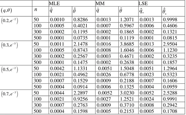
We compare the performance of these estimators in terms of their biases and mean square errors (MSEs). In Tables 5 and 6, we report the biases and MSEs of these estimators for some parameter values.

Table 5. Biases of MLE, MM and LSE estimators for some parameter values of q and o MLE MM LSE

( )

q

,

q

n

qˆ oˆ q

o

q

ˆ

_*

_o

ˆ

*

(

2

)

0.2, e 50 0.0049 0.1418 0.0094 0.3012 0.0062 0.1792 100 0.0031 0.0744 0.0055 0.1583 0.0034 0.9998 300 0.0009 0.0285 0.0016 0.0514 0.0010 0.0328 500 0.0005 0.0121 0.0009 0.0279 0.0004 0.0132

(

5

)

0.3, e 50 ₁₀₀ 0.0056 _0.0027 0.3738 _0.1727 0.0096 _0.0047 0.6610 0.0054 _{0.3166 0.0027} 0.4207 _0.1967 300 0.0008 0.0504 0.0015 0.0987 0.0008 0.0604 500 0.0005 0.0293 0.0008 0.0541 0.0003 0.0286

(

2

)

0.5, e 50 ₁₀₀ 0.0037 _0.0023 0.0942 _0.0693 0.0115 _0.0071 0.2540 -0.0003 0.0583 _{0.1622 0.0008 0.0577} 300 0.0019 0.0370 0.0034 0.0673 0.0016 0.0362 500 0.0003 0.0151 0.0013 0.0342 0.0002 0.0146

(

_{0.7, e}-3

)

50 ₁₀₀ 0.0041 _0.0034 0.3270 _0.1880 0.0117 _0.0072 0.5562 -0.0016 0.2687 _{0.3040 0.0012 0.1668} 300 0.0005 0.0465 0.0018 0.0859 0.0004 0.0427 500 0.0005 0.0306 0.0014 0.0535 0.0001 0.0294

Table 6. MSEs of MLE, MM and LSE estimators for some parameter values of q and o

MLE MM LSE

( )

q,q

n

qˆ oˆ q

o

q

ˆ

*

o

ˆ

_*

(

_{0.2, e}-2

)

50 ₁₀₀ 0.0010 _0.0005 0.8286 _0.4021 0.0013 _0.0007 1.2071 0.0013 _{0.5967 0.0006} 0.9998 _0.4606 300 0.0002 0.1195 0.0002 0.1865 0.0002 0.1321 500 0.0001 0.0735 0.0001 0.1119 0.0001 0.0815

(

5

)

0.3, e 50 ₁₀₀ 0.0011 _0.0005 2.1478 _0.8743 0.0016 _0.0008 3.8685 0.0013 _{1.6046 0.0006} 2.9504 _1.1230 300 0.0002 0.2567 0.0003 0.4671 0.0002 0.3235 500 0.0001 0.1475 0.0002 0.2638 0.0001 0.1857

(

2

)

0.5, e 50 ₁₀₀ 0.0042 _0.0021 1.1331 _0.4962 0.0051 _0.0026 1.5048 0.0051 _{0.6778 0.0023} 1.2964 _0.5323 300 0.0007 0.1529 0.0009 0.2188 0.0007 0.1606 500 0.0004 0.0914 0.0006 0.1325 0.0004 0.0959

(

3

)

0.7, e 50 ₁₀₀ 0.0044 _0.0021 2.2897 _0.9256 0.0052 _0.0027 3.0230 0.0052 _{1.2521 0.0024} 2.5288 _0.9991 300 0.0007 0.2763 0.0009 0.3710 0.0008 0.2942 500 0.0004 0.1598 0.0005 0.2153 0.0005 0.1708

From Tables 5 and 6, we see that all estimators are biased but asymptotically unbiased. The MLE and the LSE are almost identical in terms of MSE and both performs better than MM. Also, as the sample size n increases, the bias and MSE of the estimators reduce as expected.

6. APPLICATION

models:

1. Discrete Weibull (DW) distribution of Nakagawa and Osaki [15] with the pmf: ( 1)

( ; , , ) x x ; 0,1, 2,..., 0, 0 1.

DW

f x pa g ;p a -p + a x; a> < < p

2. Exponentiated discrete Weibull (EDW) of Nekoukhou and Bidram [16] with the pmf:

( 1)

( ; , , ) (1 x ) (1 x ) ; 0,1, 2,..., 0, 0, 0 1.

EDW

f x pα γ = −p + α γ − −p α γ x= α> γ > < < p

3. Discrete generalized exponential (DGE) distribution of Nekoukhou et al. [17] with the pmf:

1 1

( ; , ) x (1 x) , 1, 2,..., 0, 0 1,

DGE

f xα p =kp − −p α− x= α > < < p

4. Geometric distribution with the pmf: 1

( ; ) (1 ) x , 1, 2,..., 0 1,

Ge

f x p = −p p − x= < < p

5. Zero-truncated Poisson (ZTP) distribution with the pmf Eq. (2).

6. Discrete Poisson-Lindley (DPL) of Sankaran [18] distribution with the pmf

(

) (

)

3

2

( ; ) 2 / 1x ; 1, 2,..., 0.

DPL

f x o ;o o+ +x o+ + x; a>

The MLE, maximized log-likelihood, AIC (Akaike Information Criterion) and Kolmogorov-Smirnov (K-S) values are calculated for all models.

1. First real data set: Table 7 contains the number of failures in a certain time interval (of equal length) given and analyzed by Xie and Lai [19].

Table 7. The number of failures in a certain time interval (of equal length) Time No of failures Time No of failures Time No of failures

1 53 7 22 13 13 2 29 8 16 14 5 3 29 9 18 15 5 4 36 10 8 16 4 5 13 11 22 17 1 6 25 12 11 18 1

The summary of calculations is given in Table 8.

Table 8. MLE, maximized



, AIC, and K-S values of the fitted models for the first data set

Model MLE

−



( )

θ

ˆ

AIC K-S

GZTP _qˆ;0.7904,

_{o ;}

ˆ

_0.3100

835.2550 1674.5 0.1255

DW pˆ;0.9579,

a ;

ˆ

1.5861

851.0519 1706.1 0.4720

EDW pˆ;0.9581,

a ;

ˆ

1.5881

, g ;ˆ 0.9979 851.0519 1708.1 0.1213

Ge pˆ;0.8335 841.1116 1684.2 0.8335

ZTP _{l ;}ˆ _5.9914 996.0346 1994.1 0.4720

DPL _{o ;}ˆ _0.2940 867.1458 1736.3 0.2693

As we see from the results, the GZTP q

( )

,o model has an AIC value less than other models even less than the EDW model with having the three parameters. Further, the K-S value of the new model is better than that of other models, except the K-S value of the EDW. In discrete distributions, the K-S statistic is usually calculated without its p-value (see, e.g., Nekoukhou and Bidram, [16]; Almalki and Nadarajah, [20]; Chakraborty and Chakraborty, [21]). Indeed, a less K-S value indicates a better fit among others. Empirical cdf plots for the fitted models are given in Figure 5.

Figure 4. The first data: Empirical cdf plots for the fitted models

2. Second real data set: The data are rank frequencies of graphemes in Slovene language given in Table 3 of Makcutek [22] and have been also analyzed by Nekoukhou et al. [17]. The data are given in Table 9.

Table 9. Rank frequencies of graphemes in Slovene language

i _{f i}

( )

i _{f i}

( )

i _{f i}

( )

i _{f i}

( )

i _{f i}

( )

1 32036 6 16088 11 13034 16 7446 21 2606 2 31891 7 16084 12 10517 17 6413 22 2554 3 31122 8 15221 13 10514 18 5361 23 2463 4 27150 9 14668 14 10216 19 5055 24 1675 5 22905 10 14043 15 9568 20 4608 25 497 N=313735

The results are given in Table 10. The AIC values and Figure 6 indicate that GZTP q

( )

,o model has a better fit than other models. Further, the K-S value of the new model is better than that of other models, except the K-S value of the EDW. Finally, using the first and the second data sets, we conclude that the proposed model works well in application, especially in modelling discrete data.

Table 10. MLE, maximized



, AIC, and K-S values of the fitted models for the second data set

Model MLE

−



( )

θ

ˆ

AIC K-S

GZTP _{qˆ;0.8378, o ;}ˆ _0.3228 9.3114x105 18623x106 0.0960 DW pˆ;0.9626, ˆa ;1.4739 9.4503x105 1.8901x106 0.1005 EDW pˆ;0.8517, ˆa ;1.0407, ˆg ;1.9099 9.4394x105 1.8879x106 0.0887 DGE a ;ˆ 1.3950, ˆp;0.8808 9.4396x105 1.8879x106 0.2858 Ge pˆ;0.8715 9.3638x105 1.8728x106 0.8814 ZTP _{l ;}ˆ _7.7787 9.2318x106 2.4635x106 0.5062 DPL _{o ;}ˆ _0.2940 9.5294x106 1.9059x106 0.3060

Figure 5. The second data: Empirical cdf plots for the fitted models 7. CONCLUDING REMARKS

In this paper, a new two-parameter discrete model with an increasing hazard rate function is introduced. The new model is obtained by compounding a geometric distribution with a zero-truncated Poisson distribution with a simple structure. In fact, the new model is obtained by considering maximum of N iid

geometric random variables, where N has a zero-truncated Poisson distribution, with applications in

parallel discrete systems. The basic statistical and mathematical properties are studied in this paper. Potentiality of the new model is indicated with the good results using the two real data sets. To complete this work, one can consider the minimum of the geometric random variables with applications in series discrete systems in reliability.

CONFLICTS OF INTEREST

No conflict of interest was declared by the authors.

REFERENCES

[1] Adamidis, K., Loukas, S., "A lifetime distribution with decreasing failure rate", Statistics and Probability Letters, 39: 35-42, (1998).

[2] Barreto-Souza, W., Morais, A.L., Cordeiro, G.M., "The Weibull-geometric distribution." Journal of Statistical Computation and Simulation, 81(5): 645-657, (2011).

[3] Hemmati, F., Khorram, E., Rezakhah, S., "A new three-parameter ageing distribution",

Journal of

Statistical Planning and Inference

, 141: 2266-2275, (2011).

[4] Lu, W., Shi, D., "A new compounding life distribution: The Weibull-Poisson distribution."

Journal of

Applied Statistics,

39: 21-38, (2012).

[5] Kuş, C., "A new lifetime distribution",

Computational Statistics and Data Analysis,

51: 4497-4509, (2007).

[6] Tahmasbi, R., Rezaei, S., "A two-parameter lifetime distribution with decreasing failure rate."

Computational Statistics and Data Analysis,

52: 3889-3901, (2008).

[7] Kemp, A.W., "Classes of discrete lifetime distributions",

Communications in Statistics-Theory

and Methods

33: 3069-3093, (2004).

[8] Shafaei N.M., Rezaei, R.A.H., Mohtashami, B.G.R., "Some discrete lifetime distributions with

bathtub-shaped hazard rate functions",

Quality Engineering,

25: 225-236, (2013).

[9] Akdoğan, Y., Kuş, C., Asgharzadeh, A., Kınacı, I., Sharafi, F., "Uniform-geometric distribution."

Journal of Statistical Computation and Simulation, 86(9): 1754-1770, (2016).

[10] Gomez - Deniz, E., "A new discrete distribution: properties and applications in medical care", Journal of Applied Statistics, 40: 2760-2770, (2013).

[11] Nakagawa, T., Zhao, X., "Optimization Problems of a Parallel System with a Random Number of Units", IEEE Transactions on Reliability, 61: 543-548, (2012).

[12] Keilson, J., H. Gerber, H., "Some results for discrete unimodality." Journal of the American Statistical

Association, 66: 386-389, (1971).

[13] Braden, B., "Calculating sums of infinite series", The American Mathematical Monthly, 99(7):

649-655, (1992).

[14] Ferguson, T.S., A course in large sample theory, London: Chapman and Hall. (1996).

[15] Nakagawa, T., Osaki, S., 1975. "The discrete Weibull distribution”, IEEE Transactions on Reliability,

24: 300-301, (1975).

[16] Nekoukhou, V., H. Bidram, H., "The exponentiated discrete Weibull distribution", SORT, 39: 127-146, (2015).

[17] Nekoukhou, V., Alamatsaz, M.H., Bidram. H., "A discrete analogue of the generalized exponential

distribution", Comm. Statist. Theory Methods, 41: 2000-2013, (2012).

[18] Sankaran, M., “The discrete Poisson-Lindley distribution”, Biometrics, 26, 145-149, (1970).

[19] Xie, M., Lai, C.D., "Reliability analysis using an additive Weibull model with bathtub-shaped failure

rate function", Reliability Engineering and System Safety, 52: 87-93, (1995).

Transactions on Reliability, 63, 68-80, (2014).

[21] Chakraborty, S., Chakraborty, D., “Discrete gamma distributions: Properties and parameter estimations”, Communications in StatisticsTheory and Methods, 41, 3301-3324, (2012).

[22] Makcutek, J., "A generalization of the geometric distribution and its application in quantitative