Estımatıng the effect of ınflatıon on stock returns usıng regımedependent ımpulse response analysıs

(1)

1 SOSYAL BİLİMLER DERGİSİ

JOURNAL OF SOCIAL SCIENCES Cilt 2 Sayı 2 | Kış 2017 Volume 2 No 2 | Winter 2017, 1-16

ESTIMATING THE EFFECT OF INFLATION ON STOCK RETURNS USING REGIME-DEPENDENT IMPULSE RESPONSE ANALYSIS

Atilla ÇİFTER1*

Abstract

This study investigates the effect of inflation on stock market in South Africa with regime-dependent impulse response analysis. Nonlinear regime-dependent interaction is tested with the Markov switching vector au-toregression approach between July, 1995 and July, 2017. The results show that there is a negative impact of inflation in the short-term, and that a long-term relationship does not exist. This indicates that common stocks cannot be a hedge against inflation. The other findings relate to regime dependency and nonlinear correlation. I also found that movements of stock market are strongly regime-dependent. These results are robust in controlling additional macroeconomic variables.

Keywords: Stock market, Fisher hypothesis, regime-dependent impulse response analysis, Markov switch-ing vector autoregression.

Kısa Özet

Bu Çalışma, rejim bağımlı etki-tepki analizi ile enflasyonun Güney Afrika hisse senetleri üzerindeki etkisini araştırmaktadır. Doğrusal olmayan rejim bağımlı ilişki Markov değişim vektör otoregresyon yaklaşımıyla Tem-muz, 1995 ve Temmuz 2017 arasında test edilmiştir. Sonuçlar, enflasyonun kısa vadede negatif etkisinin oldu-ğunu ve uzun vadeli bir ilişki bulunmadığını göstermektedir. Bu bulgu, hisse senetlerinin enflasyondaki de-ğişime karşı bir önlem olamayacağını göstermektedir. Diğer bulgular rejim bağımlılığı ve doğrusal olmayan korelasyon ile ilgilidir. Bu sonuçlar ek makroekonomik değişkenlerin kontrolünde de tutarlılık göstermektedir. Anahtar Kelimeler: Hisse senedi piyasası, Fisher hipotezi, rejim bağımlı etki-tepki analizi, Markov değişim vek-tör otoregresyon.

1. Introduction

Fisher (1930) firstly argued that the change in inflation should affect the nominal interest rates. The rela-tionship between inflation and interest rates is generalized to the assets market, so that stocks can pro-vide a hedge to changes in inflation. In this content, stock returns are expected to be positively affected by rise in inflation. If the market is efficient and reflects all information, expected nominal return of stocks will rise with the inflation rate since expected nominal return should be equal to expected real return plus expected inflation. In contrast to this hypothesis, there are many empirical studies that have shown no significant correlation or negative correlation between stock returns and inflation (Lintner, 1975; Bodie, 1976; Nelson, 1976; Jaffe and Mandelker, 1976; and Fama and Schwert, 1977). Fama (1981) and Geske and Roll (1983) explained the negative relationship between stock returns and inflation with the coun-tercyclical monetary policy. Their first hypothesis is that there is a negative movement between inflation

* Altınbaş University, School of Business Administration, atilla.cifter@altinbas.edu.tr, http://works.bepress.com/atilla_cifter/ I would like to thank the external reviewers for valuable suggestions.

(2)

2

ATİLLA ÇİFTER

and economic activity, and in the second stage, there is a positive relationship between real economic activity and stock returns.

Fama (1981) and Geske and Roll (1983)’s hypothesis of long-run positive relationship between inflation and stock returns is also explained with different time horizons. Boudoukh and Richardson (1993) inves-tigated the relationship at one-year (short-term) and five-year (long-term) horizons by using the IV tech-nique. They claimed that stock returns and inflation are nearly uncorrelated with a one-year horizon; on the other hand, stock returns and inflation are positively correlated with a five-year horizon. They con-cluded that stocks can be a hedge against inflation in the long-term. Kim and In (2005) used the wave-let multi-scaling method to analyze the linkage between stock returns and inflation at short, medium, and long horizons. They found that there is a positive relationship between stock returns and inflation at a one-month and 128-month periods, while a negative relationship is shown at 2 to 128 month periods. This shows that common stocks can be a hedge against inflation in the medium horizons. Given these conflicting results, Fisher hypothesis should be tested for short, medium and long runs.

There are few studies on the relationship between stock returns and inflation in South Africa. Maghy-ereh (2006) investigated the long-term relationship between stock returns and inflation in 18 develop-ing countries with the nonparametric cointegration test. His study found evidence of a nonlinear long-term relationship in 13 out of 18 developing countries, including South Africa. Using the instrumental variables (IV) approach, Alagidede (2009) found that the Fisher hypothesis did not hold in South Africa in either the short- or long-term. Alagidede and Panagiotidis (2010) employed parametric and nonpara-metric cointegration procedures to investigate this relationship for African countries. They found that the response of stock prices to innovations in consumer prices exhibits a transitory negative response in the short-term, which becomes a positive response over longer horizons.

Unlike previous studies, Hondroyiannis and Papapetrou (2006) and Cifter (2015) used the Markov re-gime-switching vector autoregression model (MS-VAR) to analyze the effect of expected and unexpected inflation on stock returns. Hondroyiannis and Papapetrou (2006) found evidence that real stock returns are not related to expected and unexpected inflation. Rather, they found that stock market movements are regime-dependent. Cifter (2015) investigated the relationship between stock returns, inflation, and real activity for South Africa and Mexico using the Markov-switching dynamic regression approach. He uses only two regimes as recession and expansion periods. He found that there is negative relationship between inflation and stock returns in only recession period for both of the developing countries. In this paper, same as Hondroyiannis and Papapetrou (2006) and Cifter (2015), I use the MS-VAR model to estimate the Fisher equation for stock returns. But unlike these studies, I compare standard VAR and MS-VAR impulse response analyses with three regime shifts for South Africa. The short- and long-term effects of inflation on stock returns are analyzed with the VAR and MS-VAR approaches. Regime shifts in the mean and heteroskedasticity (MSMH-VAR) are estimated, and three regimes are estimated as repre-senting recession, moderate, and an expansion period. Therefore, this study differs from previous stud-ies by investigating regime switching behavior of stock market with three regimes rather than two re-gimes. In addition to the number of regimes, I use regime impulse responses analysis.

(3)

JOURNAL OF SOCIAL SCIENCES

The MS-VAR model was developed by Krolzig (1997), based on Hamilton’s (1989) univariate Markov-switch-ing autoregression model. On the basis of the MS-VAR model, the regime-dependent impulse responses can be estimated as well as regime shifts. Ehrmann et al. (2003) and Krolzig (2006) developed impulse response analysis in MS-VAR models. Krolzig’s (2006) analysis fully reflects the Markov property of the switching regimes, so this paper uses Krolzig’s (2006) impulse response analysis for regime shocks in the MS-VAR model.

The reminder of this paper is organized as follows: in the next section, the MS-VAR model’s methodol-ogy is explained. The data and empirical results are discussed in section 3. The robustness check section is presented in section 4, and the summary and some concluding remarks are presented in section 5.

2. Methodology

Sims (1980) developed the vector autoregression model (VAR) to capture the linkage between multiple time series. This is the most flexible and easy model for analyzing multiple time series, as it is an exten-sion of the univariate autoregressive model to the dynamic multivariate case (Zivot and Wang, 2006). Al-though the vector autoregression model often provides superior forecasts to the univariate time series, it has inadequate forecast performance in the presence of structural breaks. The Markov-switching vec-tor auvec-toregressive (MS-VAR) process can be an alternative to the linear VAR model because it allows mul-tiple structural breaks. The Markov-switching approach was introduced by Hamilton (1989) for formaliz-ing the statistical identification of the “turnformaliz-ing points” of a time series. This approach is an extension of Neftci’s (1984) second-order Markov process (Hamilton, 1989).

The typical behavior of the Markov process can be explained with a first-order autoregression (Hamil-ton, 1989):

t t

t

c

y

=

₁

+

φ

₋₁

+

ε

, (1)

where

c

₁ is the constant term,

φ

is the slope coefficient with εt ~N(0,σ2) and observed data 0 ,..., 3 , 2 ,1 t

t = . If there exists a significant structural break at date

t

0, this can be described as

(Hamil-ton, 2008): t t t

c

y

=

₁

+

φ

₋₁

+

ε

(2) t t t

c

y

=

₂

+

φ

₋₁

+

ε

_,

where

c

₂ is the constant term after the structural break at date

t

0. Fixing the value of the constant term

from

c

₁ to

c

₂ can improve forecast if there is only one structural break in a time series. But it is rather unsatisfactory as it does not consider a probability law between states. For this reason, the dummy riable that represents the structural break would not be adequate for most of the macroeconomic va-riables. Regime changes can be estimated with the multiple states as

s

k. The two-state Markov chain

can be shown as:

ij k k k k k js i s k P s js i p s P{ = −1 = , −2 = ,...}= { = −1 = }= (3)

(4)

4

ATİLLA ÇİFTER

where

p

ij is the probability of moving state i to state j and

p

ij

=

1 −

p

ii (when

i ≠

j

).

If

s

k follows a two-state Markov chain with transition probabilities, this can be shown as:

[

]

[

]

[

]

[

s s

]

q q s s p s s p s s k k k k k k k k − = = = = = = − = = = = = = − − − − 1 1 0 Pr 1 1 Pr 1 0 1 Pr 0 0 Pr 1 1 1 1 , (4)

where

s

k

=

0

represents recession regime, and

s

k

=

1

represents expansion regime.

Hamilton (1989) applied the MS model on U.S. real GNP growth with the following regime switching:

t s t s t s t s t t t

y

u

y

t t t t

+

−

+

−

+

−

+

−

=

−

− − − − − − − −

)

(

)

(

)

(

)

(

* 4 * 3 * 2 * 1 2 2 3 3 4 4 1 1

µ

φ

µ

φ

µ

φ

µ

φ

µ

₍₅₎

with

u

t

~ d

i

.

i

.

N

(

0 ,

σ

2

)

and with

s

*t presumed to follow a two-state Markov chain with

transi-tion probabilities.

The general form of the Markov switching regression model is defined as (Krolzig, 2000):

t p t p t t t

v

s

A

y

A

y

u

y

=

(

)

+

1 −1

+

...

+

−

+

(6)

with

u

t

s

t

~

N

(

0 ,

Σ

(

s

t

))

.The parameter shift functions

v

(

s

t

)

,

A

1

(

s

t

),...,

A

p

(

s

t

)

and

Σ

(

s

t

)

describe the dependence of the parameters on the realized regime,

s

t.

A VAR with regime shifts in the mean and heteroskedasticity is estimated with Krolzig’s (1998) approach. This model is called an MSMH (M)-VAR (p) process and can be defined as (Krolzig, 1998):

t k t k t k t

s

A

y

s

u

y

−

=

∆

−

+

∆

µ

(

)

(

₋

µ

(

₋

))

(7)

))

(

,

0 (

~

_t t t

s

N

s

u

Σ

In this paper, as suggested by Hondroyiannis and Papapetrou (2006), the MSMH-VAR is estimated with three regimes, representing recession, moderate, and expansion.

The long-term estimation of the Fisher effect can be expressed as:

t t t

t

s

CPI

u

(5)

where Stock is the logarithmic return of stock price indexes, CPI is the logarithmic return of consumer price indexes, and

s

t is states (recession, moderate, and expansion).

A two variable Markov-switching VAR model can be expressed as:

t k t k k t k k t t

s

Stock

CPI

u

Stock

=

α

(

₋

)

+

β

₋

+

λ

₋

+

(9)

Multiple variables Markov-switching VAR model for the robustness check can be expressed as:

t k t k k t k k t k k t k k t

t

s

Stock

CPI

Fx

GOLD

u

Stock

=

α

(

₋

)

+

β

₋

+

λ

₋

+

λ

₋

+

λ

₋

+

(10)

where Fx is the logarithmic return of foreign exchange rates, GOLD is the logarithmic return of gold pri-ces. Before the VAR analysis, the unit root properties of series should be checked. If the variables are non-stationary (I(0)), the bidirectional causality should be tested using the cointegration tests. Since the bi-directional causality between two variables should be tested, I use Engle and Granger (1987)’s residual based cointegration test.

3. Data and Empirical Findings 3.1. Data

In order to test the regime-dependent Fisher hypothesis, this study uses the data set of monthly consu-mer price index (CPI), FTSE JSE All Share Index (Stock), and robustness check variables as USD/ZAR fore-ign exchange rate (Fx) and gold price (GOLD). South African economy is highly dependent to gold price and this is an adequate indicator for growth of the economy. I selected foreign exchange rate as additi-onal macro variable in line with arbitrage pricing theory (APT) developed by Ross (1976).

Stock is from Johannesburg Stock Exchange (https://www.jse.co.za/), GOLD is from https://www.inves-ting.com/, and CPI and Fx are from the World Bank database. The dataset covers 265 observations from July 1995 to July 2017. Figure 1 shows nominal values and log-returns of the series. Table 1 summarizes descriptive statistics of the log-return series. Skewness statistics suggest that stock returns is negatively skewed and the inflation rate is positively skewed. Kurtosis statistics suggest that both series are lepto-kurtic, or fat-tailed. The Jarque-Bera (Jarque and Bera, 1980) test shows that all of the series including ro-bustness check variables are are not normally distributed. Standard deviation statistics show that stock returns are much more volatile than the inflation rate, as theoretically expected.

(6)

6

ATİLLA ÇİFTER

1 Figure 1 Stock and CPI

Figure 2

Fit of Three-regime MSMH(3)-VAR(1) Model for Stock Returns

4

Table 1

Descriptive Statistics

Robustness Check Variables

Stock CPI Fx GOLD

Mean 0.009 0.004 0.004 0.004 Median 0.010 0.004 0.001 0.001 Maximum 0.131 0.023 0.200 0.152 Minimum -0.351 -0.007 -0.114 -0.198 Std. Dev. 0.054 0.004 0.045 0.047 Skewness -1.211 0.675 0.619 -0.066 Kurtosis 9.853 4.127 4.528 4.124 Jarque-Bera Probability 581.261 0.000 34.038 42.603 14.098 0.000 0.000 0.000 Observations 264 264 264 264 Table 2

Unit Root Test Statistics of the Time Series

Nominal values Log-returns

ADF ADF-GLS ADF ADF-GLS

Variables t-statistics t-statistics t-statistics t-statistics

Stock 0.715 2.434 -16.785*** -16.388***

CPI 1.886 1.544 -11.690*** -10.569***

Fx -1.069 0.471 -15.813*** -15.710***

Gold -0.540 0.266 -18.345*** -18.337***

Notes. Tests contain a constant but not a time trend. The number of lags (nl) is selected with the Schwarz criteria with a maximum of twelve lags. *, **, *** indicate significance at the 10%, 5%, and 1% respectively.

(7)

Vector autoregression (linear VAR) and Markov-switching vector autoregression (MS-VAR) can be applied to stationary data. In other words, the time series should contain no unit root. Besides, stationarity sho-uld be checked for bidirectional causality. I use augmented Dickey-Fuller (ADF, Dickey and Fuller, 1981) and the GLS-trending augmented Dickey-Fuller (ADF-GLS, Elliot et al., 1996) unit root tests. The ADF-GLS is a superior unit root test in terms of size and power. Table 2 reports the unit root tests for nominal va-lues and returns. The series are non-stationary with the nominal vava-lues but stationary with the log-returns. Therefore, cointegration test can be applied to non-stationary series to test bidirectional causa-lity. Table 3 shows that stock and CPI are not cointegrated; therefore, we can conclude that the causality from CPI to stock should not be investigated and linear VAR and MS-VAR models are set with log-returns.

4 Table 1 Descriptive Statistics

Robustness Check Variables

Stock CPI Fx GOLD

Mean 0.009 0.004 0.004 0.004 Median 0.010 0.004 0.001 0.001 Maximum 0.131 0.023 0.200 0.152 Minimum -0.351 -0.007 -0.114 -0.198 Std. Dev. 0.054 0.004 0.045 0.047 Skewness -1.211 0.675 0.619 -0.066 Kurtosis 9.853 4.127 4.528 4.124 Jarque-Bera Probability 581.261 0.000 34.038 42.603 14.098 0.000 0.000 0.000 Observations 264 264 264 264 Table 2

Unit Root Test Statistics of the Time Series

Nominal values Log-returns

ADF ADF-GLS ADF ADF-GLS

Variables t-statistics t-statistics t-statistics t-statistics Stock 0.715 2.434 -16.785*** -16.388*** CPI 1.886 1.544 -11.690*** -10.569*** Fx -1.069 0.471 -15.813*** -15.710*** Gold -0.540 0.266 -18.345*** -18.337***

Notes. Tests contain a constant but not a time trend. The number of lags (nl) is selected with the Schwarz criteria with a maximum of twelve lags. *, **, *** indicate significance at the 10%, 5%, and 1% respectively.

5

Table 3

Engle-Granger Cointegration Tests

Value p-Value* Stock Engle-Granger tau-statistics -2.451 0.303 Engle-Granger z-statistics -11.087 0.296 CPI Engle-Granger tau-statistics -2.452 0.303 Engle-Granger z-statistics -10.810 0.311

Notes: * Mackinnon (1996) p-value.

Table 4

Lag Structure Criteria for the VAR

Lag Final prediction error Akaike information criterion Schwarz information criterion Hannan-Quinn information criterion 0 6.39e-08 -10.88955 -10.86185 -10.87841 1 5.75e-08* -10.99565* -10.91256* -10.96223* 2 5.91e-08 -10.96778 -10.82929 -10.91208 3 5.89e-08 -10.97132 -10.77745 -10.89335 4 5.97e-08 -10.95804 -10.70877 -10.85779 5 5.91e-08 -10.96856 -10.66389 -10.84602 6 5.96e-08 -10.95986 -10.59981 -10.81505 7 5.91e-08 -10.96774 -10.55229 -10.80065 8 5.97e-08 -10.95887 -10.48803 -10.76950

(8)

8

ATİLLA ÇİFTER

3.2. Empirical Findings

In this section, the Fisher relationship between stock returns and inflation rate is tested with linear VAR and MS-VAR models. In the first step, both vector autoregression models require lag length selection. Fol-lowing Akaike’s (1974) information criteria, a lag length of one is selected for the linear VAR and MS-VAR models a presented in Table 4. Since three regimes determine the regime dependency more accurately, the MSMH(3)-VAR(1) model is estimated for Markov switching vector autoregression.

5 Table 3

Engle-Granger Cointegration Tests

Value p-Value* Stock Engle-Granger tau-statistics -2.451 0.303 Engle-Granger z-statistics -11.087 0.296 CPI Engle-Granger tau-statistics -2.452 0.303 Engle-Granger z-statistics -10.810 0.311 Notes: * Mackinnon (1996) p-value.

Table 4

Lag Structure Criteria for the VAR

Lag Final prediction error Akaike information criterion Schwarz information criterion Hannan-Quinn information criterion 0 6.39e-08 -10.88955 -10.86185 -10.87841 1 5.75e-08* -10.99565* -10.91256* -10.96223* 2 5.91e-08 -10.96778 -10.82929 -10.91208 3 5.89e-08 -10.97132 -10.77745 -10.89335 4 5.97e-08 -10.95804 -10.70877 -10.85779 5 5.91e-08 -10.96856 -10.66389 -10.84602 6 5.96e-08 -10.95986 -10.59981 -10.81505 7 5.91e-08 -10.96774 -10.55229 -10.80065 8 5.97e-08 -10.95887 -10.48803 -10.76950

Notes: * indicates lag order selected by the criterion.

Table 5 reports the maximum likelihood estimation of the MSMH-VAR and linear VAR models and Figure 2 shows the fit of the three-regime MSMH(3)-VAR(1) model for stock returns. The result of the linear VAR model is similar with the MSMH-VAR model. According to the linear VAR model, constant term and CPI parameters are statistically significant at the 5% significance level, but not stock. The MSMH-VAR model shows that both stock and CPI, regime 2 (moderate) and regime 3 (expansion) parameters are statisti-cally significant at the 5% significance level, but not regime 1 (recession). On the other hand, regime 1 (recession)’s statistical significance is very close to 10% significance level. This indicates that stock mar-ket movements are strongly regime-dependent.

(9)

6 Table 5

Maximum Likelihood Estimation of the MSMH-VAR and OLS Estimates for the Linear VAR

MSMH-VAR Linear VAR

Dependent Variable Stocks Stocks

Regime 1 -0.028 (-1.565) - Regime 2 0.013*** (3.720) - Regime 3 0.045*** (3.634) - Constant - 0.017*** (3.491) Stock (-1) -0.156*** (2.637) -0.050 (0.821) CPI (-1) -1.534** (2.421) -1.561** (2.160) Log-likelihood 1497.069 396.568

Notes: The numbers in parenthesis are the t-statistics.*, **, *** indicate significance at the 10%, 5%, and 1% respectively.

1 Figure 1 Stock and CPI

Figure 2

(10)

10

ATİLLA ÇİFTER

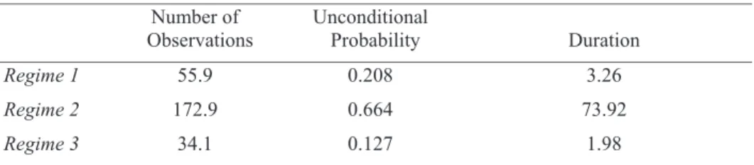
Table 6 shows the number of observations, unconditional probabilities, and durations for three regimes. Regime 2 has the highest number of observations, the highest unconditional probability, and the hig-hest duration, which is approximately 74 months. Regime duration is between two and 74 months. So that that the stock market is strongly regime-dependent for the South African stock market. This indica-tes that regimes have different structures, and linear models may not be adequate for the stock returns-inflation relationship.

7

Table 6

Regime Properties of the MSMH-VAR Model

Number of

Observations Unconditional Probability Duration

Regime 1 55.9 0.208 3.26

Regime 2 172.9 0.664 73.92

Regime 3 34.1 0.127 1.98

Table 7

Contemporaneous Correlations between Stock and CPI

Correlation coefficient

Regime 1 -0.228

Regime 2 0.048

Regime 3 -0.630

Table 7 reports contemporaneous correlations between stock returns and inflation. The figures suggest that the correlation between stock returns and inflation are different across regimes. Regime dependent correlation analysis indicates that there is a negative correlation between stock returns and inflation in the recession and expansion period and positive correlation in the moderate period. The negative cor-relation is about 23% for regime 1 and %63 for regime 3, and the positive corcor-relation is about 5% for regime 2. This shows that inflation negatively affects stock returns in extreme periods in South Africa.

7

Table 6

Regime Properties of the MSMH-VAR Model

Number of

Regime 1 55.9 0.208 3.26

Regime 2 172.9 0.664 73.92

Regime 3 34.1 0.127 1.98

Table 7

Contemporaneous Correlations between Stock and CPI

Regime 1 -0.228

Regime 2 0.048

Regime 3 -0.630

Figure 3 shows the impulse response function of the linear VAR model. Although stock returns are ne-gatively affected by inflation for up to six months, this evidence is not statistically significant, as it can be seen with bands of statistical errors. According to the standard vector autoregression approach with impulse response analysis, inflation does not affect stock returns in either the short-term or long-term. Using the instrumental variables (IV) approach, Alagidede (2009) found a similar result, that stocks can-not be a hedge for inflation. Since the linear VAR and instrumental variables (IV) approaches are from the linear platform, these results might have occurred because of the insufficiency of the selected models.

(11)

2 Figure 3

Impulse Response Function of Linear VAR Model

Figure 4

Impulse Response Functions of MSMH(3)-VAR(1) Model

Regime-dependent impulse responses using the MSMH(3)-VAR(1) model are shown in Figure 4. There is a negative relationship between stock returns and inflation for up to one month, and this negative ef-fect is corrected in approximately four months. The empirical findings indicate that impulse response functions of linear VAR model and MSMH-VAR model results are different.

2

Figure 3

Impulse Response Function of Linear VAR Model

Figure 4

Impulse Response Functions of MSMH(3)-VAR(1) Model

4. Robustness Check

In previous section, I found that impulse response function of the linear VAR model is not appropriate to investigate Fisher effect. The arbitrage pricing theory (APT) developed by Ross (1976) states that the

(12)

12

ATİLLA ÇİFTER

macroeconomic variables should be included in the regression analysis for the determinants of stock re-turns. The APT mainly uses industrial production, interest rates, inflation rates, exchange rates, default risk, money growth, gold prices, and term structure of interest rates. I selected two additional macroe-conomic variables as Fx and GOLD.

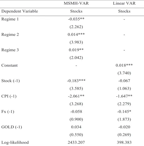
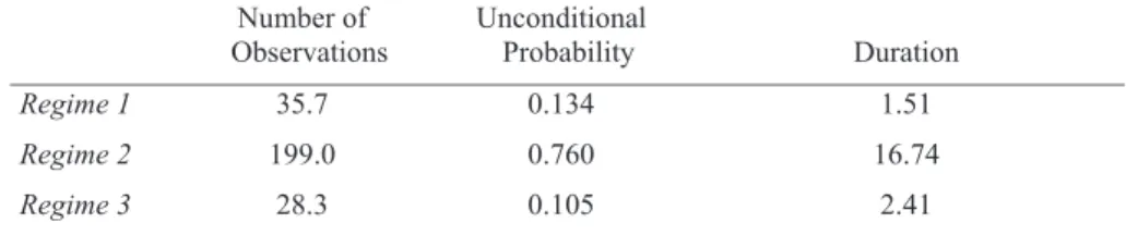
Table 8 reports the maximum likelihood estimation of the MSMH-VAR and linear VAR models with ad-ditional macroeconomic variables. The results is similar with the estimation without adad-ditional macroe-conomic variables except the significance of the Regime 1 (recession) coefficient. Regime 1 (recession)’s coefficient became significant with additional macroeconomic variables. Table 9 shows the number of observations, unconditional probabilities, and durations for three regimes, and Table 10 reports contem-poraneous correlations between stock returns and inflation. The results are similar with the previous sec-tion that the stock market is strongly regime-dependent, and the correlasec-tion between stock returns and inflation are different across regimes.

8 Table 8

Maximum Likelihood Estimation of the MSMH-VAR and OLS Estimates for the Linear VAR (Robustness Check)

MSMH-VAR Linear VAR

Dependent Variable Stocks Stocks

Regime 1 -0.035** (2.262) - Regime 2 0.014*** (3.983) - Regime 3 0.019** (2.042) - Constant - 0.018*** (3.740) Stock (-1) -0.183*** (3.585) -0.067 (1.063) CPI (-1) -2.061** (3.268) -1.647** (2.279) Fx (-1) -0.058 (0.900) -0.145* (1.873) GOLD (-1) 0.034 (0.550) -0.020 (0.269) Log-likelihood 2433.207 398.383

Notes: The numbers in parenthesis are the t-statistics.*, **, *** indicate significance at the 10%, 5%, and 1% respectively.

(13)

9 Table 9

Regime Properties of the MSMH-VAR Model (Robustness Check) Number of

Regime 1 35.7 0.134 1.51

Regime 2 199.0 0.760 16.74

Regime 3 28.3 0.105 2.41

Table 10

Contemporaneous Correlations between Stock and CPI (Robustness Check) Correlation coefficient Regime 1 -0.581 Regime 2 0.178 Regime 3 -0.196 9 Table 9

Regime Properties of the MSMH-VAR Model (Robustness Check)

Number of

Regime 1 35.7 0.134 1.51

Regime 2 199.0 0.760 16.74

Regime 3 28.3 0.105 2.41

Table 10

Contemporaneous Correlations between Stock and CPI (Robustness Check)

Regime 1 -0.581

Regime 2 0.178

Regime 3 -0.196

Figure 5 shows the impulse response function of the linear VAR model and Figure 6 shows regime-de-pendent impulse responses using the MSMH(3)-VAR(1) model. Impulse response functions are also simi-lar with the previous section, and this indicates that our results are robust in controlling additional mac-roeconomic variables.

3

Figure 5

Impulse Response Function of Linear VAR Model (Robustness Check)

Figure 6

(14)

14

ATİLLA ÇİFTER

3

Figure 5

Impulse Response Function of Linear VAR Model (Robustness Check)

Figure 6

Impulse Response Functions of MSMH(3)-VAR(1) Model (Robustness Check)

5. Conclusions

This paper investigates the effect of inflation on stock returns with regime-dependent impulse response analysis. Nonlinear regime-dependent interaction is tested with the Markov switching vector autoreg-ression model, and linear interaction is tested with the linear vector autoregautoreg-ression model. For this pur-pose, regime shifts in the mean and heteroskedasticity vector autoregression (MSMH-VAR) and linear VAR models are estimated. Three regimes are selected, representing a recession, a moderate, and an expan-sion period. The empirical findings indicate that linear VAR model and MSMH-VAR model results are dif-ferent. The MSMH-VAR model shows that there is a negative relationship between stock returns and inf-lation in the short-term, while no long-term reinf-lationship exists. The negative effect of infinf-lation appears for up to one month, and it is corrected in four months.

The other findings relate to regime dependency and nonlinear correlation. The MSMH-VAR model shows that stock market movements are strongly regime-dependent. Besides, regime-dependent correlation analysis shows that there is a negative correlation between stock returns and inflation in the recession and expansion period, while there is a positive correlation in the moderate period. This shows that infla-tion negatively affects stock returns in extreme periods in South Africa. If this evidence is valid for other stock markets, all the linear analysis becomes insufficient since linear models do not consider regime-dependent correlation.

(15)

References

Akaike, H. “A new look at the statistical model identification.” IEE Transactions on Automatic Control, 19(6) (1974): 716-723.

Alagidede P. “Relationship between stock returns and inflation.” Applied Economics Letters. 16(14) (2009): 1403-1408.

Alagidede P. and Panagiotidis, T. “Can common stocks provide a hedge against inflation? Evidence from African Countries.” Review of Financial Economics. 19(3) (2010): 91-100.

Bodie, Z. “Common Stocks as a Hedge Against Inflation.” Journal of Finance. 27 (1976): 459-470.

Boudoukh, J. and Richardson, M. “Stock returns and inflation, A long horizon perspective.” American Eco-nomic Review. 83 (1993): 1346-1355.

Cifter, A. “Stock Returns, Inflation, and Real Activity in Developing Countries: A Markov-Switching Ap-proach.” Panoeconomicus, 62(1) (2015): 55-76.

Dickey, A.D. and Fuller A.W. “ Likelihood ratio statistics for an autoregressive time series with a unit root.” Econometrica, 49 (1981): 1057-72.

Ehrmann, M., Ellison, M. and Valla, N. “Regime-dependent impulse response functions in a markov-switch-ing vector autoregressive model.” Economic Letters, 78 (2003): 295–299.

Elliott, G., Rothenberg, T.J. and Stock, J.H. “Efficient tests for an autoregressive unit root.” Econometrica, 64 (1996): 813–836.

Engle, R.F., and Granger, C.W.J. “Cointegration and error correction: representation, estimation and test-ing.” Econometrica, 55 (1987): 251–276.

Fama, E.F. “Stock Returns, Real Activity, Inflation and Money.” American Economic Review. 71 (1981): 545-565. Fama, E.F. and Schwert G.W. “Asset Returns and Inflation.” Journal of Financial Economics. 5 (1977): 115-146. Fisher, I. The Theory of Interest. New York: Macmillan, 1930.

Geske, R. and Roll, R. “The Fiscal and Monetary Linkage between Stock Returns and Inflation.” Journal of Finance, 38 (1983): 1-38.

Hamilton, J.D. “A New Approach to the Economic Analysis of Nonstationary Time Series and the Business Cycle.” Econometrica, 57(2) (1989): 357-384.

Hamilton, J.D. Regime Switching Models. S.N. Durlauf and L.E. Blume (Ed.). The New Palgrave Dictionary of Economics. Hampshire, Palgrave Macmillan, 2008.

Hondroyiannis, G. and Papapetrou, E. “Stock returns and inflation, A markov switching approach.” Review of Financial Economics. 15 (2006): 76-94.

(16)

16

ATİLLA ÇİFTER

Jaffe, F. and Mandelker, G. “The “Fisher Effect” for Risky Assets, An Empirical Investigation.” Journal of Fi-nance, 31 (1976): 447-458.

Jarque, C.M. and Bera, A.K. “Efficient tests for normality, homoscedasticity and serial independence of re-gression residuals,” Economics Letters, 6 (3) (1980): 255–259.

Kim, S. and In, F. “The Relationship between Stock Returns and Inflation, New Evidence from Wavelet Anal-ysis.” Journal of Empirical Finance, 12 (2005): 435-444.

Krolzig, H.M. Econometric modeling of Markov-switching vector autoregressions using MSVAR for Ox. Discussion Paper, Department of Economics, University of Oxford, 1998.

Krolzig, H.M. Predicting Markov-Switching Vector Autoregressive Processes. Oxford University. Working Paper 2000W31, 2000.

Krolzig, H.M. Markov Switching Vector Autoregression. Modelling, Statistical Inference and Application to Busi-ness Cycle Analysis. Berlin: Springer, 1997.

Krolzig, H.M. Impulse-Response Analysis in Markov Switching Vector Autoregressive Models. Economics Department. University of Kent. Keynes College, 2006.

Lintner, J. “Inflation and Security Returns.” Journal of Finance. 30 (1975): 259-280.

Maghyereh. A. “The long-run relationship between stock returns and inflation in developing countries, Further evidence from a nonparametric cointegration test.” Applied Financial Economics Letters. 2 (2006): 265-273.

Neftçi, S.. “Are Economic Time Series Asymmetric Over the Business Cycle?.” Journal of Political Economy, 92 (1984): 307-328.

Nelson, C.R. “Inflation and Rates of Return on Common Stocks.” Journal of Finance, 31 (1976): 471-483. Sims, C.A. “Macroeconomics and Reality.” Econometrica, 48(1) (1980): 1-48.

Ross, S. “The arbitrage theory of capital asset pricing.” Journal of Economic Theory. 13(3) (1976): 341–360. Zivot, E. and Wang, J. Modeling Financial Time Series with S-PLUS. New York: NY,Springer Science+Busi-ness Media, 2006.