ISTANBUL KULTUR UNIVERSITY
NUMERICAL METHODS FOR PARTIAL DIFFERENTIAL EQAUTIONS
SERHAT YILMAZ
MA THESIS
ISTANBUL KULTUR UNIVERSITY INSTITUTE OF SCIENCE
DEPARMENT OF MATHEMATICS AND COMPUTER
NUMERICAL MTHDS
NAME AND SURNAME: Serhat YILMAZ REGISTRATION NUMBER: 0809041044
ABSTRACT
NUMERICAL METHODS FOR PARTIAL DIFFERENTIAL EQUATIONS
Numerical methods are used to find an approximation solution to problems in practice of science and engineering are often either diffucult or imppossible to solve analytically. In this study, we deal to find numerical solutions of some kinds of partial differential
equations(PDE). PDE are used to formulate, and thus aid the solution of, problems involving functions of severable variables; such as the propagation of sound or heat, electrostatics, electrodynamics, fluid flow, and elasticity. Seemingly, distinct physical phenomena may have identical mathematical formulations, and thus be governed by the same underlying dynamic. Here, we develop numerical hybrid methods to solve PDE. The first method based on non-poylnomial cubic splines in the space direction and finite difference in the time direction. We have seen by using spline functions additional smoothness can be achieved. In the second method we use finite elements methods with Galerkin method instead of splines in the space direction but ıt gives a heavy calculation and not beter results. Several numerical techniques have been proposed fort he numerical solution of PDE. These tecniques are compared giving by numerical examples, and all numerical results are illustrated using MATLAB 7.0.
KEYWORDS: Partial differential equations, Numeric methods, Collection methods, Non-polynomial cubic splines, Finite element methods, Galerkin methods.
ÖZET
KISMİ TÜREVLİ DİFERANSİYEL
DENKLEMLERİN SAYISAL
ÇÖZÜMLERİ
Numerik metodlar fizik ve mühendislik uygulamalarında ortaya çıkan ve çözümü çok zor veya mümkün olmayan problemler için yaklaşım çözümleri üretmek için kullanılır. Bu çalışmada, biz parçalı diferansiyel denklemlere sayısal çözümler bulunmasına odaklandık. Kısmi türevli diferansiyel denklemler(PDE) birkaç bilinmeyen değişkene bağlı fonksiyonlar içeren
problemleri formülize etmekte ve tabii ki çözümlerinde kullanılmaktadır. PDE, Isı dağılımı, elektrostatik, elektrodinamik, akışkan dinamiği gibi farklı fizik problemlerinde karşımıza çıkarlar.
Bu çalışmada, PDE'i çözmek için sayısal hibrid metodlar gelişdirdik. İlk metot, uzay boyutunda polinom olmayan kübik splineların, zaman boyutunda ise sonlu farkların
kullanılması üzerine inşa edilmiştir. İkinci metotda ise uzay boyutunda splineların yerine sonlu elamanlar Galerkin metoduyla birlikte kullanılmıştır. Sonuç olarak splineların daha yakınsak bir sonuç verdiği, buna karşılık sonlu fark metodunun hem daha ağır hesaplamalar gerektirdiği hem de daha iyi olmayan sonuçlar verdiği görülmüşdür. Farklı metotlar bizim metodumuzla sayısal örnekler verilerek kıyaslanmıştır. Sayısal çözümlerin hepsi MATLAB 7.0 kullanılarak hesaplanmışdır.
ANAHTAR KELİMELER VE SÖZCÜKLER: Parçalı diferansiyel denklemler, Sayısal Metodlar, Kolakasyon metodları, polinom olmayan splinelar, Sonlu Elemanlar, Galerkin metod.
Acknowledgements
Contents
abstract . . . .
iii
Acknowledgements . . . .
v
Sections
1 introduction . . . .
1
2 Partial Differential Equations . . . .
2
2.1 Preliminaries . . . 2
2.2 Classification . . . 3
2.3 Associated conditions . . . 4
3 Collocation . . . .
7
3.1 Introduction . . . 7
3.2 Non-polynomial Cubic Splines . . . 8
3.3 B-splines . . . 35
4 Finite Element Method . . . 37
4.1 Introduction . . . 37
5 Conclusion . . . 39
5.1 compare . . . 39
References . . . 40
Chapter 2
Partial Differential Equations
2.1
Preliminaries
A partial differential equation (PDE) describes a relation between an unknown func-tion and its partial derivatives. PDEs appear frequently in all areas of physics and engineering. Moreover, in recent years we have seen a dramatic increase in the use of PDEs in areas such as biology, chemistry, computer sciences (particularly in relation to image processing and graphics) and in economics (finance). In fact, in each area where there is an interaction between a number of independent variables, we attempt to define functions in these variables and to model a variety of processes by construct-ing equations for these functions. When the value of the unknown function(s) at a certain point depends only on what happens in the vicinity of this point, we shall, in general, obtain a PDE. The general form of a PDE for a function u(x1, x2, ..., xn)
is F (x1, x2, ..., xn, u, ux1, ux2, ..., ux11, ...) =0, where x1, x2, ..., xn are the independent
variables, u is the unknown function, and uxi denotes the partial derivative du/dxi.
The equation is, in general, supplemented by additional conditions such as initial conditions (as we have often seen in the theory of ordinary differential equations (ODEs)) or boundary conditions.
The analysis of PDEs has many facets. The classical approach that dominated the nineteenth century was to develop methods for finding explicit solutions. Because of the immense importance of PDEs in the different branches of physics, every mathe-matical development that enabled a solution of a new class of PDEs was accompanied by significant progress in physics. Thus, the method of characteristics invented by Hamilton led to major advances in optics and in analytical mechanics. The Fourier
method enabled the solution of heat transfer and wave propagation, and Greens methodwas instrumental in the development of the theory of electromagnetism. The most dramatic progress in PDEs has been achieved in the last 50 years with the introduction of numerical methods that allow the use of computers to solve PDEs of virtually every kind, in general geometries and under arbitrary external conditions (at least in theory; in practice there are still a large number of hurdles to be overcome).
2.2
Classification
We can say that PDEs are often classified into different types. In fact, there exist several classifications. Some of them will be describedin this section.
The first classification is according to the order of the equation. The order is defined to be the order of the highest derivative in the equation. If the highest derivative is of order k, then the equation is said to be of order k. Thus, for example, the equation
utt− uxx = f (x, t) is called a second-order equation, while ut+ uxxxx= 0 is called a
fourth-order equation.
Another classification is into two groups: linear versus nonlinear equations. An equa-tion is called linear if in (1.1), F is a linear funcequa-tion of the unknown funcequa-tion u and its derivatives. Thus, for example, the equation x3u
x+ eyuy+ sin(x2+ y2)u = x4 is a
linear equation, while u2
x+ u2y = 1 is a nonlinear equation. The nonlinear equations
are often further classified into subclasses according to the type of the nonlinearity. Generally speaking, the nonlinearity is more pronounced when it appears in a higher derivative. For example, the following two equations are both nonlinear:
uxx+ uyy = u2 (1.2)) uxx+ uyy =|∇u|2u. (1.3)
Here |∇u| denotes the norm of the gradient of u. While (1.3) is nonlinear, it is still linear as a function of the highest-order derivative. Such a nonlinearity is called quasi-linear. On the other hand in (1.2) the nonlinearity is only in the unknown function. Such equations are often called semilinear.
Here we have to mention that there is a classification of the family of second-order linear equations for functions in two independent variables into three distinct types: hyperbolic (e.g., the wave equation), parabolic (e.g., the heat equation), and elliptic equations (e.g., the Laplace equation). It turns out that solutions of equations of the
same type share many exclusive qualitative properties.Also by a certain change of variables any equation of a particular type can be transformed into a canonical form which is associated with its type. An equation that has the form
L[u] = auxx+ buxy + cuyy+ dux+ euy + f u = g, (1.4)
where a, b, . . . , f, g are given functions of x, y, and u(x, y) is the unknown function. We assume that the coefficients a, b, c do not vanish simultaneously.The operator L0[u] = auxx+ buxy+ cuyy that consists of the second-(highest-)order terms
of the operator L is called the principal part of L. It turns out that many fundamental properties of the solutions of (1.4) are determined by its principal part, and, more precisely, by the sign of the discriminant δ(L) := b2−4ac of the equation. We classify the equation according to the sign of δ(L).Equation (1.4) is said to be hyperbolic at a point (x, y) if δ(L)(x, y) > 0,it is said to be parabolic at (x, y) if δ(L)(x, y) = 0, and it is said to be elliptic at (x, y) if δ(L)(x, y) < 0.
Finally, a single PDE with just one unknown function is called a scalar equation. In contrast, a set of m equations with l unknown functions is called a system of m equations.
2.3
Associated conditions
PDEs have in general infinitely many solutions. In order to obtain a unique solution one must supplement the equation with additional conditions. What kind of condi-tions should be supplied? It turns out that the answer depends on the type of PDE under consideration. In this section we briefly review the common conditions. Let us consider the convection equation Ct+ ⃗∇ • (C⃗u) = 0 in one spatial dimension
as a prototype for equations of first order. The unknown function C(x, t) is a sur-face defined over the (x, t) plane. It is natural to formulate a problem in which one supplies the concentration at a given time t0, and then to deduce from the equation
the concentration at later times. Namely, we solve the problem consisting of the convection equation with the condition C(x, t0) = C0(x). This problem is called an
initial value problem. Geometrically speaking, condition determines a curve through which the solution surface must pass. We can generalize this condition by imposing a curve Γ that must lie on the solution surface, so that the projection of Γ on the (x,
t) plane is not necessarily the x axis. The last example involve PDEs with just a first derivative with respect to t. In analogy with the theory of initial value problems for ODEs, we expect that equations that involve second derivatives with respect to t will require two initial conditions. Therefore it is natural to supply two initial conditions, one for the initial location , and one for its initial velocity:
u(x, 0) = u0(x), ut(x, 0) = u1(x).
Another type of constraint for PDEs that appears in many applications is called boundary conditions. As the name indicates, these are conditions on the behavior of the solution (or its derivative) at the boundary of the domain under consideration. As an example, consider the heat equation with a spatial domain Ω:
ut = k(uxx+ uyy+ uzz) (x, y, z)∈ Ω, t > 0. (1.45)
We shall assume in general that Ω is bounded. It turns out that in order to obtain a unique solution, one should provide (in addition to initial conditions) information on the behavior of u on the boundary ∂Ω. Excluding rare exceptions, we encounter in applications three kinds of boundary conditions. The first kind, where the values of the temperature on the boundary are supplied, i.e.
u(x, y, z, t) = f (x, y, z, t) (x, y, z)∈ Ω, t > 0, (1.46)
is called a Dirichlet condition in honor of the German mathematician Johann Leje-une Dirichlet (1805.1859). For example, this condition is used when the boundary temperature is given through measurements, or when the temperature distribution is examined under a variety of external heat conditions. Alternatively one can supply the normal derivative of the temperature on the boundary; namely, we impose
∂nu(x, y, z, t) = f (x, y, z, t) (x, y, z)∈ Ω, t > 0, (1.46)
This condition is called a Neumann condition after the German mathematician Carl Neumann (1832.1925). We have seen that the normal derivative ∂nu describes the
flux through the boundary. For example, an insulating boundary is modeled by con-dition (1.47) with f = 0.
A third kind of boundary condition involves a relation between the boundary values of u and its normal derivative: α(x, y, z) + ∂nu(x, y, z, t) + u(x, y, z, t) = f (x, y, z, t)
(x, y, z)∈ Ω, t > 0, (1.46)
Such a condition is called a condition of the third kind. Sometimes it is also called the Robin condition.
Although the three types of boundary conditions defined above are by far the most common conditions seen in applications, there are exceptions. For example, we can
supply the values of u at some parts of the boundary, and the values of its normal derivative at the rest of the boundary. This is called a mixed boundary condition. Another possibility is to generalize the condition of the third kind and replace the nor-mal derivative by a (smoothly dependent) directional derivative of u in any direction that is not tangent to the boundary. This is called an oblique boundary condition. Also, one can provide a nonlocal boundary condition. For example, one can provide a boundary condition relating the heat flux at each point on the boundary to the integral of the temperature over the whole boundary.
Chapter 3
Collocation
3.1
Introduction
Let X be a linear subspace of L2[D],the space of square integrable functions on D,
where D is some subset of the real line E1 or of the real plane E2.And, Let L be a linear operator whose domain is X and whose range is also in X. Let {Φ1, Φ2,...,ΦN
be a linearly independent subset of X, and let XN = span{Φ1, Φ2, ..., ΦN} be an
N-dimensional subspace of X. Suppose we are given the linear equation:
Lx = y, (3.1)
where y is given function from X. Approximating the solution x(t) of (3.1) by the method of collocation consists of finding a function xN(t) = a1Φ1(t) + a2ϕ2(t) + ... +
anϕN(t) in XN solving the N × N system of linear equations
LxN(ti) = N
∑
j=1
ajLϕj(ti) = y(ti), 1 ≤ i ≤ N, (3.2)
where t1, t2, ...tN are N distinct points of D at which all the terms of (2) are defined.
The function xN(t), if it exists, is said to collocate y(t) at the points t1, t2, ...tN. Any
function f(t) so obtained is referred to as an approximate solution obtained by the method of collocation.
In the following sections, we use method of collocation with non-polynomial cubic splines and with b-splines.
3.2
Non-polynomial Cubic Splines
Consider the polynomial interpolation, that is using approximations based on the idea of finding a polynomial which agrees with, or interpolates, the data and using this polynomial in place of the original function to estimate its values at other points. The use of local polynomials clearly improved the performance but at he expense of smoothness in the approximating function. However, additional smoothness can be achived with local polynomial interpolation by using spline functions in which different low-degree polynomials are used on each interval [xi, xi+1] together with the
imposition of smoothness conditions to ensure that the overall interpolating function has high a degree of continuity as possible at each of the nodes, xi.
Definition 3.2.1. Let x0 < x1 < ... < xN be an increasing sequence of nodes. The function s is a spline function of degree k if:
(a) s is a polynomial of degree no more than k on each of the subintervals [xi, xi+1].
(b) s, s′,...,sk−1 are all continous on the interval [xi, xi+1].
By far the most commonly used splines for interpolation purposes are the cubic splines, and it is on these that we will concentrate our attention. The cubic spline functions have the form span{1, x, x2, x3 . In the present section, we apply non-polynomial cubic spline functions that have a non-polynomial and trigonometric parts to develop numerical methods for obtaining smooth approximations to the solution of partial differential equations. The spline functions we propose in this section have the form span , x, coskx, sinkx where k is the frequency of the trginometric part of the spline functions which will be used to raise the accuracy of the method.
We turn now to the specific problem of obtaining a nonpolynomial cubic spline func-tion which interpolates the fucfunc-tion f at x0, x1, ..., xN.
Let u(x) be a function defined on [a, b]. We divide the interval [a, b] into n equal subintervals using the grid points
xi = a + ih, i = 0, 1, 2, ..., n,
with
where n is an arbitrary positive integer.
Let u(x) be the exact solution and ui be an approximation to u(xi) obtained by the
non-polynomial cubic Si(x) passing through the points (xi, ui) and (xi+1, ui+1), we
do not only require that Si(x) satisfies interpolatory conditions at xi and xi+1, but
also the continuity of first derivative at the common nodes (xi, ui) are fulfilled. We
write Si(x) in the form:
Si(x) = ai+ bi(x− xi) + cisinτ (x− xi) + dicosτ (x− xi), i = 0, 1, ..., n− 1 (3.3)
where ai, bi, ci and di are constants and τ is a free parameter.
A non-polynomial function S(x) of class C2[a, b] interpolates u(x) at the grid points xi, i = 0, 1, 2, ..., n, depends on a parameter τ , and reduces to ordinary cubic
spline S(x) in [a, b] as τ → 0.
To derive expression for the coefficients of Eq. (3.3) in term of ui, ui+1, Mi and
Mi+1, we first define:
Si(xi) = ui, Si(xi+1) = ui+1, S
′′
(xi) = Mi, S
′′
(xi+1) = Mi+1. (3.4)
From algebraic manipulation, we get the following expression:
ai = ui+ M i τ2 , bi = ui+1− ui h + Mi+1− Mi τ θ , ci = Micosθ− Mi+1 τ2sinθ , di = −Mi τ2 , where θ=τ h and i = 0, 1, 2, ..., n− 1.
Using the continuity of the first derivative at (xi, ui), that is S
′
i−1(xi) = S
′
i(xi) we
obtain the following relations for i=1, ..., n− 1.
aMi+1+ bMi+ aMi−1 = (1/h2)(ui+1− 2ui+ ui−1) (3.5)
where a = (−1/θ2+ 1/θ sin θ), b = (1/θ2− cos θ/θ sin θ) and θ = τh. The method is
fourth-order convergent if b = 5/12 and a = 1/12 [9]. We next develop approximations for some examples:
Example 3.2.2. Firstly we consider the second-order linear hyperbolic equation:
utt(x, t) + 2αut(x, t) + β2u(x, t) = uxx(x, t) + f (x, t), x∈ (a, b), t > 0 (3.6) with initial conditions
u(x, 0) = Φ(x), ut(x, 0) = Ψ(x) and boundary conditions
u(a, t) = g1(t), u(b, 0) = g2(t)
where α and β are constants.
The equation above represents a damped wave equation and a telegraph equation, the existence and approximations of the solutions investigated, see[1].
In recent years, many research has been done in developing and implementing modern high resolutions methods for the numerical solution of the second-order linear hyperbolic equation(1), see[1− 3]. Mohanty and Jain[4 − 5] and Mohanty[6] developed three-level implicit schemes for linear hyperbolic equations. Recently, Gao and Chi[7] proposed two semi-discretion methods to solve the one-space dimensional linear hy-perbolic equation(1). Also, Huan-Wen Liu and Li-Bin Liu solved[8] linear hyhy-perbolic equation. In this paper, we propose a non-polynomial cubic spline difference scheme to solve the linear hyperbolic equation(1). For every xi, i = 1, 2, ..., n− 1, by using the Taylor expansion in the time direction, we have the following difference schemes
u(xi, tj) = u(xi, tj+1) + 2u(xi, t) + u(xi, tj−1)
4 + O(k 2 ), (3.7) uxx(xi, tj) = uxx(xi, tj+1) + uxx(xi, tj−1) 2 + O(k 2), (3.8) ut(xi, tj) = u(xi, tj+1)− u(xi, tj−1) 2k + O(k 2), (3.9) utt(xi, tj) =
u(xi, tj+1)− 2u(xi, tj) + u(xi, tj−1)
k2 + O(k
The given eq. (1) can be discretized as
u(xi, tj+1)− 2u(xi, tj) + u(xi, tj−1) k2
+2αu(xi, tj+1)− u(xi, tj−1) 2k
+β2u(xi, tj+1) + 2u(xi, t) + u(xi, tj−1) 4
= uxx(xi, tj+1) + uxx(xi, tj−1)
2 + f (xi, tj) + O(k
2). (3.11)
i = 1, 2, ..., n− 1, j = 1, 2, ...
We can rewrite (3.5) in a new form :
(1 + 1 12δ 2 x)M (xi, tj) = 1 h2δ 2 xu(xi, tj), i = 1, ..., n− 1 (3.12) where δxM (xi, tj) = M (xi+12, tj)− M(xi−1 2, tj),
δx2M (xi, tj) = δx(δxM (xi, tj)) = M (xi+1, tj)− 2M(xi, tj) + M (xi−1, tj) for i = 1, ..., n− 1. Putting (3.8) and (3.12),it follows that;
(1 + 1 12δ 2 x)[uxx(xi, tj+1) + uxx(xi, tj−1)] = (1 + 1 12δ 2 x)[M (xi, tj+1) + M (xi, tj−1) + O(h4)] = 1 h2δ 2
x[u(xi, tj+1) + u(xi, tj−1)] + O(h4) (3.13) Applying the operator (1 +121 δ2
x) to two sides of Eq. (3.11) and using Eq. (3.13),then it is obtained as follows 1 k2(1 + 1 12δ 2 x)u(xi, tj) + α k(1 + 1 12δ 2 x)δtu(xi, tj) +β 2 4 (1 + 1 12δ 2
x)[u(xi, tj+1+ 2u(xi, tj) + u(xi, tj−1)]
− 1 2h2δ 2 x[u(xi, tj+1)u(xi, tj−1)] = (1 + 1 12δ 2 x)f (xi, tj) + O(k 2 + h4)i = 1(1)n− 1, j = 1, 2, ... (3.14)
The proposed scheme (3.14) is an implicit three level scheme. To start any computa-tion, it is necessary to know the value of u(x, t) at the nodal points of the first time level, that is, at t = k. Following [12],a taylor series expansion at t=k may be written as u(x, k) = u(x, 0) + kut(x, 0) + k2 2 utt(x, 0) + k3 6 uttt(x, 0) + O(k 4). (3.15)
Using the initial values, from (1) we can calculate
utt(x, 0) = ϕxx(x, 0) + f (x, 0)− 2αut(x, 0)− β2u(x, 0), (3.16)
uttt(x, 0) = ψxx(x, 0) + ft(x, 0)− 2tt(x, 0)− β2ut(x, 0). (3.17) We can obtain the numerical solution of u by using initial values in(3.16) and (3.17) for t = k.
Now let us consider a specific equation:
utt(x, t) + 4ut(x, t) + 2u(x, t) = uxx(x, t), x∈ (a, b), t > 0 (3.18) with initial conditions
u(x, 0) = sinx, ut(x, 0) =−sinx
and boundary conditions
u(0, t) = 0, u(π, 0) = 0.
The exact solution of the above problem is u(x, t) = e−tsinx. The problem is solved by using the scheme(3.14) in this paper. The absolute errors given by the scheme (16) in
[7], by the scheme (23) in [8] and by present scheme (13) are listed in Tables 3.1-3.4,
respectively. It can be seen from tables, whenh = π
300 and k = 0.1, the accuracy of
solutions obtained by using the scheme (16) in [7] is much better than those by using the present scheme(13). The reason is that the error orders of the scheme (16) in
[7] is approximately O(k5) as the step length h is quite small. When k decreases to
k = 0.1 and k = 0.01, respectively ,since k is now quite small in comparison with h, the errors of numerical solutions mainly come from the approximation in space direc-tion,therefore the absolute errors by using the present scheme(13) is much better than those by using the scheme (16) in [7]. Finally, we have to mention that the absolute errors of scheme (23) in [8] are similar to those by using the present scheme(3.14) where scheme (23) in [8] using quartic spline functions, we use non-polynomial spline functions.
Table 3.1: Absolute errors of the scheme(16) in[7], the scheme (23) in [8] and the present scheme(3.14) (h = 300π , k = 0.1).
t x = 30π x = 8π30 x = 15π30 x = 22π30 x = 29π30
[7] 1.0 0.0105e-05 0.0747e-05 0.1005e-05 0.0747e-05 0.0105e-05
[8] 1.0 0.0379e-03 0.2969e-03 0.4033e-03 0.3026e-03 0.0463e-03
[T hepresents.] 1.0 0.0429e-03 0.3056e-03 0.4112e-03 0.3056e-03 0.0429e-03
[7] 2.0 0.1015e-06 0.7215e-06 0.9709e-06 0.7215e-06 0.1015e-06
[8] 2.0 0.0389e-03 0.3039e-03 0.4128e-03 0.3096e-03 0.0475e-03
[T hepresents.] 2.0 0.0435e-03 0.3092e-03 0.4161e-03 0.3092e-03 0.0435e-03
Table 3.2: Absolute errors of the scheme(16) in[7], the scheme (23) in [8] and the present scheme(3.14) (h = 30π, k = 0.1).
t x = 30π x = 8π30 x = 15π30 x = 22π30 x = 29π30
[7] 1.0 0.0904e-04 0.6479e-04 0.8928e-04 0.7069e-04 0.0904e-04
[8] 1.0 0.0321e-03 0.6995e-03 0.2033e-03 0.6995e-03 0.0412e-03
[T hepresents.] 1.0 0.0298e-03 0.3055e-03 0.4111e-03 0.3055e-03 0.0429e-03
[7] 2.0 0.0884e-04 0.6337e-04 0.8731e-04 0.6913e-04 0.0884e-04
[8] 2.0 0.0532e-03 0.5065e-03 0.3128e-03 0.5065e-03 0.0331e-03
[T hepresents.] 2.0 0.0349e-03 0.3092e-03 0.4161e-03 0.3092e-03 0.0865e-03
Table 3.3: Absolute errors of the scheme(16) in[7], the scheme (23) in [8] and the present scheme(3.14) (h = 30π, k = 0.01).
t x = 10π x = 3π10 x = 5π10 x = 7π10 x = 9π10
[7] 1.0 0.2947e-04 0.7717e-04 0.9539e-04 0.7717e-04 0.2947e-04
[8] 1.0 0.0886e-05 0.3170e-05 0.4242e-05 0.3170e-05 0.0886e-05
The present s. 1.0 0.1320e-05 0.3456e-04 0.4272e-05 0.3456e-05 0.1320e-05
[7] 2.0 0.2883e-04 0.7548e-04 0.9330e-04 0.7548e-04 0.2883e-04
[8] 2.0 0.0871e-05 0.3114e-05 0.4167e-05 0.3114e-05 0.0871e-05
Table 3.4: Absolute errors of the scheme(16) in[7], the scheme (23) in [8] and present scheme(3.14),(h = 30π, k = 0.001).
t x = 10π x = 3π10 x = 5π10 x = 7π10 x = 9π10
[7] 1.0 0.2947e-04 0.7717e-04 0.9539e-04 0.7717e-04 0.2947e-04
[8] 1.0 0.1839e-08 0.6574e-08 0.8799e-08 0.6574e-08 0.1839e-08
The present s. 1.0 0.1096e-08 0.7134e-08 0.8819e-08 0.7134e-08 0.1096e-08
[7] 2.0 0.28834e-04 0.75489e-04 0.93309e-04 0.75489e-04 0.28834e-04
[8] 2.0 0.1799e-08 0.6433e-08 0.8609e-08 0.6433e-08 0.1799e-08
The present s. 2.0 0.1992e-08 0.7029e-08 0.8398e-08 0.7029e-08 0.1992e-08
Example 3.2.3. Secondly we consider the generalized Fisher’s equation:
ut(x, t) = uxx(x, t) + αu(x, t)(1− uβ(x, t)) a < x < b, t > 0 (3.19) with initial condition
u(x, 0) = Φ(x), and boundary conditions
u(a, t) = g1(t), u(b, t) = g2(t)
where α and β are constants.
The classic and simplest case of the nonlinear reaction-diffusion equation is when β=1. It was suggested by Fisher as a deterministic version of a stochastic model for the spatial spread of a favored gene in a population [1].
ut(x, t) = uxx(x, t) + αu(x, t)(1− u(x, t)) a < x < b, t > 0 (3.20) This equation is referred to as the Fisher equation, the discovery, investigation and analysis of traveling waves in chemical reactions was first presented by Luther [2]. In the last century, the Fisher’s equation has became the basis for a variety of models for spatial spread, for example, in logistic population growth models [3, 4], flame propa-gation [5, 6], neurophysiology [7], autocatalytic chemical reactions [8− 10], branching
Brownian motion processes [11], gene-culture waves of advance [12], the spread of early farming in Europe [13, 14], and nuclear reactor theory [15]. It is incorporated as an important constituent of nonscalar models describing excitable media, e.g., the Belousov-Zhabotinsky reaction [16]. In chemical media, the function u(x, t) is the concentration of the reactant and the positive constant α represents the rate of the chemical reaction. In media of other natures, u might be temperature or electric potential.
The mathematical properties of equation (1) have been studied extensively and there have been numerous discussions in the literature. The most remarkable sum-maries have been provided by Brazhnik and Tyson [17]. One of the first numerical solutions was presented in literature with a pseudo-spectral approach. Implicit and explicit finite differences algorithms have been reported by different authors such as Parekh and Puri and Twizell et al. A Galerkin finite element method was used by Tang and Weber whereas Carey and Shen [18] employed a least-squares finite element method. A collocation approach based on Whittakers sinc interpolation function [19] was also considered in [20]. Our solution based on non-polynomial spline method. In this paper, we propose a spline difference scheme to solve eq. (2).
Let the region R = (a, b)× (0, ∞], be discretized by a set of points Rh,k which are the vertices of a grid points (xi, tj), where xi = ih, i = 0, 1, 2, ..., n, nh = 1, and tj = jk, j = 0, 1, 2, 3. Here h and k are mesh size in the space and time directions respectively.
We develop an approximation for eq.(2) in which the time derivative is replaced by a finite difference approximation and the space derivative by the non-polynomial cubic spline function approximation. We need the following finite difference approximation for the time derivative of u. Let:
¯
ut(xi, tj) = u(xi,tj+1)−u(xi,tj−1)
2k = ut(xi, tj) + O(k
2). (7)
At the grid point (i, j), the proposed differential equation (2) may be discretized by:
¯
ut(xi, tj) = ¯uxx(xi, tj) + αu(xi, tj)(1− u(xi, tj)). (8)
u(xi,tj+1)−u(xi,tj−1)
2k = M (xi, tj)− αu(xi, tj)(1− u(xi, tj)), (9)
where M (xi, tj) = S
′′
(xi) is the second spline derivative at (xi, tj). From (9) we have
M (xi, tj) = u(xi,tj+1)2k−u(xi,tj−1) − αu(xi, tj)(1− u(xi, tj)), (10) then we have
M (xi+1, tj) = u(xi+1,tj+1)2k−u(xi+1,tj−1)− αu(xi+1, tj)(1− u(xi+1, tj)), (11) and
M (xi−1, tj) = u(xi−1,tj+1)−u(xi−1,tj−1)
2k − αu(xi−1, tj)(1− u(xi−1, tj)), (12)
substituting (10), (11) and (12) into (6), after simplifying we obtain:
λu(xi+1, tj+1) + µu(xi, tj+1) + λu(xi−1, tj+1)
+aα(u(xi+1, tj+1))2+ 2b(u(xi, tj+1))2+ aα(u(xi−1, tj+1))2 a ku(xi+1, tj−1)− 2b ku(xi, tj−1)− a ku(xi−1, tj−1) = 0 (13) where λ = ak− aα − h12, µ = 2b k − 2bα + 2 h2 and a is parameter.
4.The similar scheme with using Taylor expansion
Expanding (13) in Taylor series in terms of u(xi, tj) and its derivatives, we can obtain another scheme(17). To do this, for simplicity, let (xi, tj) denote the grid points given by xi = a + ih ,i = 0, 1, ..., n, and tj = jk, j = 0, 1, 2, ...For every xi, i = 1, 2, ..., n− 1, by using the Taylor expansion in the time direction, we have the following difference schemes
u(xi, tj) = u(xi,tj+1)+2u(xi,tj)+u(xi,tj−1)
4 + O(k
uxx(xi, tj) = uxx(xi,tj+1)+uxx(xi,tj−1) 2 + O(k 2) (15) ut(xi, tj) = u(xi,tj+1)−u(xi,tj−1) 2k + O(k 2) (16)
By using (14), (15) and (16),the given equation (2) can be discretized as
u(xi,tj+1)−u(xi,tj−1)
2k − α
u(xi,tj+1)+2u(xi,tj)+u(xi,tj−1)
4 (1−
u(xi,tj+1)+2u(xi,tj)+u(xi,tj−1)
4 )
= uxx(xi,tj+1)+uxx(xi,tj−1)
2 i = 1, ..., n− 1, j = 1, 2, ... (17)
So, (6) equality can be rewritten in a new form as follow :
(1 + 121 δ2
x)M (xi, tj) = h12δx2u(xi, tj), i = 1, ..., n− 1 (18) where
δxM (xi, tj) = M (xi+12, tj)− M(xi−1 2, tj),
δx2M (xi, tj) = δx(δxM (xi, tj)) = M (xi+1, tj)− 2M(xi, tj) + M (xi−1, tj),
for i = 1, ..., n− 1. Using (14) and (18), we have;
(1 +121δx2)[uxx(xi, tj+1) + uxx(xi, tj−1)] = (1 + 121δx2)[M (xi, tj+1) + M (xi, tj−1) + O(h4)]
=h12δ
2
x[u(xi, tj+1) + u(xi, tj−1)] + O(h4). (19)
If we apply the operator (1 + 121 δx2) to two sides of (17) and use (19), we have
1 2k(1 +
1 12δ
2
x)[u(xi, tj+1)− u(xi, tj−1)]−α4(1 + 121δ2x)[u(xi, tj+1) + 2u(xi, tj) + u(xi, tj−1)]
+ α
16(1 + 1 12δ
2
x)[u(xi, tj+1) + 2u(xi, tj) + u(xi, tj−1)]2−2h12δ
2
x[u(xi, tj+1) + u(xi, tj−1)] = 0
i = 1, 2, ..., n− 1, j = 1, 2, ... (20)
The proposed scheme (20) is an implicit three level scheme. To start any computa-tion, it is necessary to know the value of u(x, t) at the nodal points of the first time
level, that is, at t = k. Following [22], a taylor series expansion at t=k may be written as u(x, k) = u(x, 0) + kut(x, 0) + k 2 2utt(x, 0) + k3 6 uttt(x, 0) + O(k 4) (21)
Using the initial values, from (1) we can calculate
utt(x, 0) = ϕxx(x, 0) + f (x, 0)− 2αut(x, 0)− β2u(x, 0), (22) uttt(x, 0) = ψxx(x, 0) + ft(x, 0)− 2αutt(x, 0)− β2ut(x, 0), (23) Thus using initial value and (22), from (23), we may obtain the numerical solution of u at t = k.
5. Numerical example
In this section, we test our scheme on an example. All computations are done by using MATLAB 7.0.
We consider the numerical results obtained by apllying the schemes dicussed above to the following Fisher‘s equation
ut(x, t) = uxx(x, t) + 6u(x, t)(1− u(x, t)), 0 < x < 1, t > 0
with initial condition
u(x, 0) = (1+e1x)2,
and boundary conditions
u(0, t) = (1+e1−5t)2, u(1, t) =
1 (1+e1−5t)2
The exact solution of the above problem is u(x, t) = (1+ex1−5t)2. The problem is
solved by using the schemes (13) and (20) in this paper.The maximum absolute errors given by scheme (13) are listed in Table 1 and given by scheme (20) are listed in Table 2.The results prove that the second method with using Taylor expansion is more accurate than the first method in this paper.Also, numerical results given by scheme
(13) and given by scheme (20) are shown in Fig. 1 and Fig. 2, respectively.
Example 3.2.4. Hyperbolic partial differential equations play a very important role
modern applied mathematics due to their deep physical background. Hyperbolic dif-ferential equation subject to an integral conservation condition in one space dimen-siona,feature in the mathematical modelling of many phenomena. Recently, much attention has been paid in the literature to the development, analsis and implemen-tation of accurate methods.In this paper we will consider a non-classic hyperbolic equation [1]:
We consider the following problem of this family of equations:
∂u ∂t = γ
∂2u
∂x2, (x, t)∈ (0, 1) × (0, T ] (1.1)
with initial condition
u(x, 0) = f (x), 0≤ x ≤ 1, (1.2)
and boundary conditions
u(0,t)=g(t), 0≤ t ≤ T, (1.3)
∫x
0 u(x, t)dx = m(t), 0 < x≤ T, (1.4)
where g and m are known functions. u′′ + a1(x)u ′ + a2(x)u + a3(x)v ′ + a4(x)v = f1(x), v′′+ b1(x)v ′ + b2(x)v + b3(x)u ′ + b4(x)u = f2(x) ,
(1)
with the following boundary conditions
u(0) = u(1) = 0, v(0) = v(1) = 0 (2)
where ai(x), bi(x), f1(x) and f2(x) are given functions for i = 1, 2, 3, 4.
The analytical solutions of eqs. (1) and (2) have been studied by a number of authors [Lu, Abbas, Sami]. In [Lu] the variational iteration method is applied for the solutions with the assumption that the solutions are unique. In [Sami] the homo-topy analysis method (HAM) is applied for the solutions and a new modification of HAM is proposed. The comparasion between the modified HAM and standard HAM is also presented in [Sami]. Recently He’s homotopy perturbation method (HPM) is applied to the problems (1) and (2) in [Abbas]. Their method consists of reducing the solutions to a system of integral equations and using the HPM for this system. In a recent work [Caglar1], we have discussed the numerical solutions of the linear system of the second-order BVPs using the third-degree B-splines. It has been shown that the B-spline method is workable and cable of solve the the linear system of the second-order BVPs.
On the other hand, the non-polynomial spline method is also very useful and ef-fective tool and used for a large variety of problems by several authors, e.g. [is-lam,ras1,ras2,ras3]. Islam et al. [islam] considered the non-polynomial spline method for the solution of a system of second-order BVPs. Recently, Rashidinia et al. [ras1] introduced the non-polynomial spline method for the second-order hyperbolic equa-tions with mixed boundary condiequa-tions. More recently, Rashidinia et al. [ras2, ras3] have also showed that this method can be successfully implemented to the numerical solution of non-linear singular BVPs. They used the quesilinearization technique to reduce the given non-linear problem to a sequence of linear problems.
In the present work, we present a numerical solution of Eq. (1) with boundary conditions (2) by using the non-polynomial spline method. Two linear test problems
are considered for the numerical illustration of the method and numerical results are illustrated using MATLAB 6.5. We have showed that the proposed method is a full computational method and a powerful tool for solving the linear system of the second-order BVPs.
Example 3.2.5. Parabolic partial differential equations play a very important role
modern applied mathematics due to their deep physical background. Parabolic differ-ential equation with non-local boundary conditions in one, two or three space dimen-tions,feature in the mathematical modelling of many phenomena. Recently, much at-tention has been paid in the literature to the development, analsis and implementation of accurate methods.In this paper we will consider a non-classic parabolic equation [1]:
∂u ∂t = γ
∂2u
∂x2, (x, t)∈ (0, 1) × (0, T ] (1.1)
with initial condition
u(x, 0) = f (x), 0≤ x ≤ 1, (1.2)
and boundary conditions
u(0,t)=g(t), 0≤ t ≤ T, (1.3)
∫x
0 u(x, t)dx = m(t), 0 < x≤ T, (1.4)
where g and m are known functions.
As another type of non-local boundary value problem consider ∂u
∂t = γ ∂2u
∂x2 + q(x, t), (x, t)∈ (0, 1) × (0, T ], (1.5)
with initial condition (1.2) and boundary condition
u(1, t) = g(t), 0 < t≤ T, (1.6)
and non-local condition
∫b(x)
There are many papers that deal with integral conditions giving the specification of mass, e.g. Dehghan [1-3], Cannon and Matheson [4], Cannon and van der Hoek [5]. Dehgan and Tatari [1] solved this problem using the radical basis functions for discretization of space and finite difference methods for discretization of time. Also Caglar considered third degree B-spline functions to solve one-dimentional heat equa-tion [6]. In Ref. [7] a new method is proposed in the reproducing kernel space and the solution is given by the form of series. In the paper by Martin-Vaquero [10], Crandall’s formulas is used to solve second-order parabolic equation subject to non-local conditions. The author of [11] applied new finite difference schemes to solve one-dimensional parabolic equation with boundary integral conditions.
A more extensive list of references as well as a survey on progress made on this class of problems may be found in Dehghan [2]
The organization of this paper as follows:In section 2, 3 and 4, we investigate two different non-polynomial cubic spline methods. In section 5, we give two different examples of parabolic partial differential equations with non-local conditions. A con-clusion is given in Section 6. Finally some references are presented at the end.
Let the region R = (0, 1)× (0, T ], be discretized by a set of points Rh,k which are the vertices of a grid points (xi, ti), where xi = ih, i = 0, 1, 2, ..., n,nh = 1, and tj = jk, j = 0, 1, 2, 3. Here h and k are mesh size in the space and time directions respectively.
We develop an approximation for eq.(1.1) in which the time derivative is replaced by a finite difference approximation and the space derivative by the non-polynomial cubic spline function approximation. We need the following finite difference approximation for the time derivative of u. Let:
ut(xi, tj) =
u(xi, tj+1)− u(xi, tj−1)
2k = ut(xi, tj) + O(k
2) (7)
At the grid point (i,j), the proposed differential equation (1.1) may be discretized by:
ut(xi, tj) = γuxx(xi, tj) (8) By using (7) in equation (8) we obtain
u(xi, tj+1)− u(xi, tj−1)
2kγ = M (xi, tj) (9)
where M (xi, tj) = S′′(xi) is the second spline derivative at (xi, tj). From (9) we have
M (xi+1, tj) =
u(xi+1, tj+1)− u(xi+1, tj−1)
2kγ , (10)
and
M (xi−1, tj) =
u(xi−1, tj+1)− u(xi−1, tj−1)
2kγ , (11)
substituting (9),(10) and (11) into (6), after simplifying we obtain: α(u(xi+1,tj+1)−u(xi+1,tj−1)
2kγ ) + 2β(
u(xi,tj+1)−u(xi,tj−1)
2kγ ) + α(
u(xi−1,tj+1)−u(xi−1,tj−1)
2kγ )
− 1
h2(u(xi+1, tj)− 2u(xi, tj) + u(xi−1, tj)) = 0
4. The similiar scheme with using Taylor expansion
For every xi, i = 1(1)(n− 1), by using the Taylor expansion in the time direction, we have the following difference schemes
uxx(xi, tj) = uxx(xi,tj+1)+uxx(xi,tj−1) 2 + O(k 2) ut(xi, tj) = u(xi,tj+1)−u(xi,tj−1) 2k + O(k 2) (12)
The given eq. (1.1) may be discretized as u(xi,tj+1)−u(xi,tj−1) 2k = γ uxx(xi,tj+1)+uxx(xi,tj−1) 2 + O(k 2), (13) i = 1, 2, ..., n− 1, j = 1, 2, ...
So, (6) equality can be rewritten in a new form as follow:
(1 + 1 12δ 2 x)M (xi, tj) = 1 h2δ 2 xu(xi, tj), i = 1, ..., n− 1 (14) where δxM (xi, tj) = M (xi+12, tj)− M(xi−1 2, tj), δ2 xM (xi, tj) =δx(δxM (xi, tj)) = M (xi+1, tj)− 2M(xi, tj) + M (xi−1, tj),
For i = 1, ..., n− 1. Using (12) and (14), we have;
(1 +121δ2 x)[uxx(xi, tj+1) + uxx(xi, tj−1)] = (1 + 121δx2)[Sxx(xi, tj+1) + Sxx(xi, tj−1) + O(h4)] = (1 + 1 12δ 2 x)[Sxx(xi, tj+1) + Sxx(xi, tj−1)] + O(h4) = h12δ 2 x[S(xi, tj+1) + S(xi, tj−1)] + O(h4) = h12δ 2
x[u(xi, tj+1) + u(xi, tj−1)] + O(h4). (15) Applying the operator (1 + 1
12δ 2
x) to two sides of Eq. (13) and using Eq. (15), we have
u(xi+1, tj+1)(24k1 −2hγ2) + u(xi, tj+1)(2k1 − 12k1 +hγ2) + u(xi−1, tj+1)(24k1 − 2hγ2) =
u(xi+1, tj−1)(24k1 + 2hγ2) + u(xi, tj−1)( 1 2k − 1 12k − γ h2) + u(xi−1, tj−1)( 1 24k + γ 2h2) i = 1(1)(n− 1), j = 1, 2, ... (16)
The proposed scheme (16) is an implicit three level scheme. To start any compu-tation, it is necessary to know the value of u(x, t) at the nodal points of the first time
level, that is, at t = k. From Taylor series expansion at t = k may be written as
u(x, k) = u(x, 0) + kut(x, 0) + k
2
2utt(x, 0) + O(k
3
) (17)
Using the initial values, from (1.1) we can calculate
ut(x, 0) = γuxx(x, 0) (18) .
Thus using initial value and (18), from (17), we may obtain the numerical solution of u at t = k.
We need two more equations. The two end conditions can be derivated as follows
u0 = 0 (19)
h
3(u0+ 4u1+ 2u2+ 4u3+ ... + 4un−1+ un) = m(t) (20)
The method is described in matrix form for Eqs.(16),(19),(20):
A = 1 0 0 0 ... 0 0 0 (24k1 − 2hγ2) ( 5 12k + γ h2) ( 1 24k − γ 2h2) 0 ... 0 0 0 (24k1 − 2hγ2) ( 5 12k + γ h2) ( 1 24k − γ 2h2) 0 ... 0 . . . . ... . . . . . . . ... . . . . . . . ... . . . 0 0 0 0 ... (24k1 −2hγ2) ( 5 12k + γ h2) ( 1 24k − γ 2h2) 1 4 2 4 ... 2 4 1 , (45)
B= 0 -f(x1)(24k1 +2hγ2)− f(x2)(12k5 − hγ2)− f(x3)(24k1 + 2hγ2) -f(x2)(24k1 +2hγ2)− f(x3)(12k5 − hγ2)− f(x4)(24k1 + 2hγ2) . . . -f(xn−2)(24k1 + 2hγ2)− f(xn−1)( 5 12k − γ h2)− f(xn)( 1 24k + γ 2h2) 3 hm(t) , (43)
Finally we find out the approximation solution as U = [u0, u1, ..., un]′
AU = B
4. Test Examples
In this section, to illustrate our methods we have solved the boundary value problem for the one-dimentional heat equation with nonlocal initial condition. All computa-tions are done by using MATLAB 6.5.
Example 1.
We first consider the following equations
f (x) = cos(Π2x), 0 < x < 1, g(t) = exp(−Π42t), 0 < t < 1, m(t) = Π2exp(−Π42t), 0 < t < 1 (50)
with the exact solution of the above problem is u(x, t) = exp(−Π42t)cos(Π2x)
Example 3.2.6. We consider a non-linear system of second-order BVPs of the form
u′′+ a1(x)u ′ + a2(x)u + a3(x)v ′ + a4(x)v + H1(x, u, v) = f1(x), v′′+ b1(x)v ′ + b2(x)v + b3(x)u ′ + b4(x)u + H2(x, u, v) = f2(x), (1)
with the following boundary conditions
u(0) = u(1) = 0, v(0) = v(1) = 0 (2)
where 0 < x < 1, H1, H2 are nonlinear functions of u and v, ai(x), bi(x), f1(x), and
f2(x), are given functions, and ai(x), bi(x) are continuous, i = 1, 2, 3, 4.
The existence and approximations of the solutions to non-linear systems of second-order BVPs have investigated by many authors[1-6]. In [1] the sinc-collocation method is presented for solving second-order systems. Their method consists of reducing the solution of Eq.(1) to a set of algebric equations by expanding u(x) and v(x) as sinc functions with unknown coefficients. New method is presented to solve Eq.(1) used in the form of series in the reproducing kernel space in [2]. The variation iteration method is applied for the solution with the assumption that the solutions are unique in [3]. He’s homotopy perturbation method (HPM) is proposed for the solution of systems in [5]. A new modification of the homotopy analysis method (HAM) is pre-sented for solving systems of second-order BVPs in [6].
The section of this paper are organized as follows: In the next section we describe the basic formulation of the spline function required for our subsequent development. In section 3 the method are used to analysis to solution of problem (1) and (2). In section 4 some numerical result, that are illustrated using MATLAB 6.5, are given to clarify the method. Section 5 ends this paper with a brief conclusion. Note that we have computed the numerical results by MATLAB 6.5.
To illustrate the application of the Spline method developed in the previous section we consider the non-linear system of second-order BVP that is given in Eq. (1). At the grid point (xi, ui), the proposed non-linear system of second-order BVP in Eq. (1) may be discretized by
u′′+ a1(xi)u ′ + a2(xi)u + a3(xi)v ′ + a4(xi)v + H1(x, u, v) = f1(xi), v′′+ b1(xi)v ′ + b2(xi)v + b3(xi)u ′ + b4(xi)u + H2(x, u, v) = f2(xi). (7) Substituting Mi = u ′′ and Ni = v ′′ in equation system (5): Mi+ a1(xi)u ′ i+ a2(xi)ui+ a3(xi)v ′ i+ a4(xi)vi+ H1(xi, ui, vi) = f1(xi), Ni+ b1(xi)v ′ i+ b2(xi)vi+ b3(xi)u ′ i + b4(xi)ui + H2(xi, ui, vi) = f2(xi). (8)
Solving Eq. (8) for Mi and Ni, we get
Mi =−a1(xi)u ′ i− a2(xi)ui− a3(xi)v ′ i − a4(xi)vi− H1(xi, ui, vi) + f1(xi) Ni =−b1(xi)v ′ i− b2(xi)vi− b3(xi)u ′ i− b4(xi)ui− H2(xi, ui, vi) + f2(xi) (9)
The following approximations for the first-order derivative of u and v in Eq. (9) can be used
u′i ∼= ui+1−ui−1
2h ,
u′i+1∼= 3ui+1−4ui+ui−1
2h ,
u′i−1∼= −ui+1+4ui−3ui−1
2h , v′i ∼= vi+1−ui−1 2h , v′i+1∼= 3vi+1−4vi+vi−1 2h , v′i−1 ∼= −vi+1+4vi−3vi−1 2h . (10) So Eq. (9) becomes
Mi =−a1(xi)ui+12h−ui−1 − a2(xi)ui− a3(xi)vi+12h−vi−1 −a4(xi)vi− H1(xi, ui, vi) + f1(xi)
(11a)
Mi+1=−a1(xi+1)3ui+1−4u2hi+ui−1 − a2(xi+1)ui− a3(xi+1)3vi+1−4v2hi+vi−1 −a4(xi+1)vi− H1(xi+1, ui+1, vi+1) + f1(xi+1)
Mi−1=−a1(xi−1)−ui+1+4u2hi−3ui−1 − a2(xi−1)ui− a3(xi−1)−vi+1+4v2hi−3vi−1 −a4(xi−1)vi− H1(xi−1, ui−1, vi−1) + f1(xi−1) (11c) and
Ni =−b1(xi)vi+12h−vi−1 − b2(xi)vi− b3(xi)ui+12h−ui−1 −b4(xi)ui− H2(xi, ui, vi) + f2(xi)
(12a)
Ni+1 =−b1(xi+1)3vi+1−4v2hi+vi−1 − b2(xi+1)vi− b3(xi+1)3ui+1−4u2hi+ui−1 −b4(xi+1)ui− H2(xi+1, ui+1, vi+1) + f2(xi+1)
(12b)
Ni−1 =−b1(xi−1)−vi+1+4v2hi−3vi−1 − b2(xi−1)vi− b3(xi−1)−ui+1+4u2hi−3ui−1 −b4(xi−1)ui− H2(xi−1, ui−1, vi−1) + f2(xi−1)
(12c)
Substituting Eqs. (11a-11c)-(12a-12c) in Eqs. (6a) and (6b) respectively, we find the following 2(n− 1) linear algebraic equations in the 2(n + 1) unknowns for i = 0, 1, ..., n. [αa1(xi−1) 2h − 2βa1(xi) 2h − 3αa1(xi+1) 2h − αa2(xi+1)− 1 h2]ui+1 +[−4αa1(xi−1) 2h − 2βa2(xi) + 4αa1(xi+1) 2h + 2 h2]ui +[3αa1(xi−1) 2h − αa2(xi−1) + 2βa1(xi) 2h − αa1(xi+1) 2h − 1 h2]ui−1 +[αa3(xi−1) 2h − 2βa3(xi) 2h − 3αa3(xi+1)
2h − αa4(xi+1)]vi+1
+[−4αa3(xi−1) 2h − 2βa4(xi) + 4αa3(xi+1) 2h ]vi +[3αa3(xi−1) 2h − αa4(xi−1) + 2βa3(xi) 2h − αa3(xi+1) 2h ]vi−1
−αH1(xi−1, ui−1, vi−1)− 2βH1(xi, ui, vi)− αH1(xi+1, ui+1, vi+1) = −αf1(xi−1)− 2βf1(xi)− αf1(xi+1) (13) and
[αb1(xi−1) 2h − 2βb1(xi) 2h − 3αb1(xi+1) 2h − αb2(xi+1)− 1 h2]vi+1 +[−4αb1(xi−1) 2h − 2βb2(xi) + 4αb1(xi+1) 2h + 2 h2]vi +[3αb1(xi−1) 2h − αb2(xi−1) + 2βb1(xi) 2h − αb1(xi+1) 2h − 1 h2]vi−1 +[αb3(xi−1) 2h − 2βb3(xi) 2h − 3αb3(xi+1)
2h − αb4(xi+1)]ui+1
+[−4αb3(xi−1) 2h − 2βb4(xi) + 4αb3(xi+1) 2h ]ui +[3αb3(xi−1) 2h − αb4(xi−1) + 2βb3(xi) 2h − αb3(xi+1) 2h ]ui−1
−αH2(xi−1, ui−1, vi−1)− 2βH2(xi, ui, vi)− αH2(xi+1, ui+1, vi+1) = −αf2(xi−1)− 2βf2(xi)− αf2(xi+1) (14)
We need four more equations. The four end conditions can be derivated as follows: u0 = 0, un = 0, v0 = 0, vn = 0
}
(15)
This leads to the system
X1i= αa12h(xi−1)− 2βa2h1(xi) −3αa12h(xi+1)− αa2(xi+1)−h12 (16)
Y1i= −4αa2h1(xi−1) − 2βa2(xi) + 4αa12h(xi+1) +h22 (17)
Z1i= 3αa12h(xi−1) − αa2(xi−1) + 2βa2h1(xi)− αa1(x2hi+1) −h12 (18)
X2i = αa3(x2hi−1) − 2βa2h3(xi)− 3αa32h(xi+1) − αa4(xi+1) (19) Y2i = −4αa3
(xi−1)
2h − 2βa4(xi) +
4αa3(xi+1)
2h (20)
Z2i= 3αa32h(xi−1) − αa4(xi−1) + 2βa2h3(xi) − αa3(x2hi+1) (21) gi = a12h(xi) , hi = a2(xi) , ki = a32h(xi) , li = a4(xi) (22)
X1i= αgi−1− 2βgi− 3αgi+1− αhi+1− h12 (23)
Z1i= 3αgi−1+ 2βgi− αgi+1− αhi−1− h12 (25)
X2i= αki−1− 2βki− 3αki+1− αli+1 (26)
Y2i=−4αki−1+ 4αki+1− 2βli (27)
Z2i = 3αki−1+ 2βki− αki+1− αli−1 (28) X3i= αb3(x2hi−1) − 2βb2h3(xi) − 3αb32h(xi+1)− αb4(xi+1) (29) Y3i = −4αb3 (xi−1) 2h − 2βb4(xi) + 4αb3(xi+1) 2h (30) Z3i = 3αb32h(xi−1) − αb4(xi−1) + 2βb2h3(xi) −αb3(x2hi+1) (31) X4i = αb1(x2hi−1) −2βb2h1(xi) − 3αb12h(xi+1) − αb2(xi+1)− h12 (32)
Y4i= −4αb2h1(xi−1)− 2βb2(xi) + 4αb12h(xi+1)+ h22 (33)
Z4i = 3αb12h(xi−1) − αb2(xi−1) + 2βb2h1(xi)− αb1(x2hi+1)− h12 (34)
mi = b12h(xi), pi = b2(xi), ri = b32h(xi), si = b4(xi) (35)
X3i = αri−1− 2βri− 3αri+1− αsi+1 (36)
Y3i=−4αri−1+ 4αri+1− 2βsi (37)
Z3i= 3αri−1+ 2βri− αri+1− αsi−1 (38)
X4i= αmi−1− 2βmi− 3αmi+1− αpi+1−h12 (39)
Y4i=−4αmi−1+ 4αmi+1− 2βpi+ h22 (40)
The method is described in matrix form in the following way for Eqs. (16)-(41): A = A1 | A2 − − − A3 | A4 , (42) B= 0 -αf1(x0)− 2βf1(x1)− αf1(x2) -αf1(x1)− 2βf1(x2)− αf1(x3) . . . -αf1(xn−2)− 2βf1(xn−1)− αf1(xn) 0 0 -αf2(x0)− 2βf2(x1)− αf2(x2) -αf2(x1)− 2βf2(x2)− αf2(x3) . . . -αf2(xn−2)− 2βf2(xn−1)− αf2(xn) 0 , (43)
H = 0 -αH1(x0, u0, v0)− 2βH1(x1, u1, v1)− αH1(x2, u2, v2) -αH1(x1, u1, v1)− 2βH1(x2, u2, v2)− αH1(x3, u3, v3) . . . -αH1(xn−2, un−2, vn−2)− 2βH1(xn−1, un−1, vn−1)− αH1(xn, un, vn) 0 0 -αH2(x0, u0, v0)− 2βH2(x1, u1, v1)− αH2(x2, u2, v2) -αH2(x1, u1, v1)− 2βH2(x2, u2, v2)− αH2(x3, u3, v3) . . . -αH2(xn−2, un−2, vn−2)− 2βH2(xn−1, un−1, vn−1)− αH2(xn, un, vn) 0 , (44) U = [u0, u1, ..., un, v0, v1, ..., vn] ′ . (44)
Here the four submatrices A1, A2, A3 and A4 are defined as
A1 = 1 0 0 0 ... 0 0 X11 Y11 Z11 0 ... 0 0 0 X12 Y12 Z12 0 ... 0 . . . . . . . . . . . . . . . . . . . . . 0 ... 0 0 X1(n−2) Y1(n−2) Z1(n−2) . . . . 0 0 1 , (45)
A2 = 0 0 0 0 ... 0 0 X21 Y21 Z21 0 ... 0 0 0 X22 Y22 Z22 0 ... 0 . . . . . . . . . . . . . . . . . . . . . 0 ... 0 0 X2(n−2) Y2(n−2) Z2(n−2) . . . . 0 0 0 , (46) A3 = 0 0 0 0 ... 0 0 X31 Y31 Z31 0 ... 0 0 0 X32 Y32 Z32 0 ... 0 . . . . . . . . . . . . . . . . . . . . . 0 ... 0 0 X3(n−2) Y3(n−2) Z3(n−2) . . . . 0 0 0 , (47) A4 = 1 0 0 0 ... 0 0 X41 Y41 Z41 0 ... 0 0 0 X42 Y42 Z42 0 ... 0 . . . . . . . . . . . . . . . . . . . . . 0 ... 0 0 X4(n−2) Y4(n−2) Z4(n−2) . . . . 0 0 1 . (48)
Finally the approximate solution is obtained by solving the nonlinear system using Levenberg-Marquardt optimization method [7] and Matlab 6.5.
AU + H = B. (49)
In this section, to illustrate our methods we have solved two non-linear system of second-order BVP . All computations are done by using MATLAB 6.5.
Example 1.
Consider the following equations
u′′(x)− xv′(x) + u(x) = f1(x)
v′′(x) + xu′(x) + u(x)v(x) = f2(x)
(50)
subject to the boundary conditions
u(0) = u(1) = 0, v(0) = v(1) = 0, (51)
where 0 < x < 1, f1(x) = x3− 2x2 + 6x and f2(x) = x2− x.
The exact solutions of u(x) and v(x) are given as x3− x and x2− x respectively.
The observed maximum absolute errors of u(x) and v(x) for n = 21 (nodal points) are given in Table 1. The numerical results of u(x) and v(x) are also illustrated in Figures 1 and 2.
3.3
B-splines
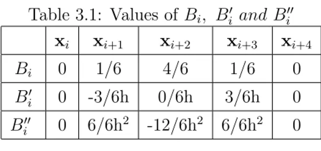
B-spline method is so named because of use of splines as basis function. In this section, we will focus on B-spline basis and their definitions. Secondly, we will look the results of this method on diffusion equation and compare them with other methods. Let Ωnbeapartitionof [a,b]⊂ ℜ. A B-spline of order k is a spline from
Sk(Ωn)withminimalsupportandthepartitionof unityholding.T oexplainthis, letusdef inedBi,j(x)wherei
![Table 3.1: Absolute errors of the scheme(16) in[7], the scheme (23) in [8] and the present scheme(3.14) (h = 300π , k = 0.1).](https://thumb-eu.123doks.com/thumbv2/9libnet/3490733.16444/20.892.195.869.230.429/table-absolute-errors-scheme-scheme-present-scheme-π.webp)
![Table 3.4: Absolute errors of the scheme(16) in[7], the scheme (23) in [8] and present scheme(3.14),(h = 30π , k = 0.001).](https://thumb-eu.123doks.com/thumbv2/9libnet/3490733.16444/21.892.203.892.228.426/table-absolute-errors-scheme-scheme-present-scheme-π.webp)