Copyright © 2019, TSI® Press Vol. 25, no. 2, 305–311
https://doi.org/10.31209/2018.100000006
CONTACT Nazan Çakmak Polat [email protected] © 2019 TSI® Press
A Method for Decision Making Problems by Using Graph
Representation of Soft Set Relations
Nazan Çakmak Polat, Gözde Yaylali, Bekir Tanay
Department of Mathematics, Faculty of Sciences, Muğla Sıtkı Koçman University, 48170, Muğla, TURKEY
KEY WORDS: Decision Making Problem, Representation of Soft Set Relations, Soft Sets.
1 INTRODUCTION
THERE are real life problems in engineering, social and medical sciences, economics etc. involving imprecise data that can be solved by mathematical principles based on uncertainty and imprecision. Most of the times, traditional methods are limited due to their uncertainties. Though theory of probability, fuzzy set theory, intuitionistic fuzzy sets, vague sets, theory of interval mathematics, rough set theory etc. may be utilized as efficient tools to deal with diverse types of uncertainties and imprecision embedded in a system, they have their inherit difficulties as pointed out by Molodtsov (1999).
Molodtsov (1999) introduced soft set theory and successfully applied it in several directions such as the smoothness of the functions, game theory, operation research, Riemann integration, Perron integration, probability, theory of measurement. Maji, Biswas and Roy (2003) studied equality of two soft sets, soft subset and soft super set of a soft set, complement of a soft set, null soft set, absolute soft set and soft binary operations. Some soft and fuzzy soft algebraic structures e.g. soft groups, soft rings, fuzzy soft moduls were also studied by many researchers (Acar, et. al. 2010; Aktaş and Çağman, 2007; Gunduz and Bayramov, 2011a, 2011b; Ozturk, Gunduz and Bayramov, 2013). The soft set relation was introduced by Babitha and Sunil (2010). In another study Babitha and Sunil (2011) transitive closures and orderings on soft sets were introduced. Later in 2012, some properties related to soft set relations were extended by Park, Kim and Kwun (2012).
Moreover, Çağman and Enginoğlu (2010) defined soft matrices, which are representation of soft sets. Out of its several advantages, one is to store and manipulate matrices, hence the soft sets can be entered in a computer.
After these advances, the soft set theory became an important mathematical tool for vagueness. Zhang (2014) introduced the Interval soft set, which is a combination of interval set and soft set, and applied the interval soft set to construct a decision making algorithm. In addition, the concept of soft intervals, whose special case is interval soft set, was defined by Tanay and Yaylalı (2015) Constructing new Decision Making Algorithms is very important for social life problems involving imprecise data. (Ballı and Turker, 2017; Wang and Wang, 2016; Zeinalova, 2014) are some recent studies on decision making methods that are based on multi-criteria decision making and decision making under Z-information.
Representing soft structures in an innovative and effective way is very important to improve the soft set theory. Herein, we have developed a new tool to visualize soft set relation using directed graphs and successfully applied it to solve decision making problems given in previous studies (Tanay and Yaylalı, 2015; Zhang, 2014). We have used some literature (Grimaldi, 2004) elementary definitions in the graph theory such as graph, subgraph etc.
2 PRELIMINARIES
LET’s recall some basic notions in the soft set theory:
ABSTRACT
Soft set theory, which was defined by D. Molodtsov, has a rich potential for applications in several fields of life. One of the successful application of the soft set theory is to construct new methods for Decision Making problems. In this study, we are introducing a method using graph representation of soft set relations to solve Decision Making problems. We have successfully applied this method to various examples.
Definition 2.1. (Molodtsov, 1999) Let Ube an initial universal set and Ebe a set of parameters. Let P U( )
denote the power set of Uand AE. A pair (F A, )
is called a soft set over U, where Fis a mapping given by F:AP U( ).
Definition 2.2. (Maji, et. al. 2003) For two soft sets
(F A, ) and (G B, ) over a common universeU, we say that (F A, ) is soft subset of (G B, ) if:
i)AB, and
ii) e A, F e( ) and G e( ) are identical approximations.
it is denoted by .
Definition 2.3. (Maji, et. al. 2003) Let (F A, ) and
(G B, ) be soft sets over a common universe U. The intersection of (F A, ) and (G B, ) is defined as the soft set (H C, ) satisfying the following conditions: i) C AB.
ii) For all xC H x, ( )F x( ) or G x( )
(while two soft sets are the same).
in this case, we can write . Definition 2.4. (Maji, et. al. 2003) Let (F A, ) and
(G B, ) be soft sets over a common universe U. The union of (F A, ) and (G B, ) is defined as the soft set
(H C, ) satisfying the following conditions: i) C AB.
ii) For all xC,
( ) , ( ) ( ) , ( ) ( ) . F x if x A B H x G x if x B A F x G x if x A B
in that case, we write . Definition 2.5. (Babitha and Sunil, 2010) Let (F A, )
and (G B, ) be soft sets over a common universe U, then the Cartesian product of (F A, ) and (G B, ) is defined as (F A, )( ,G B)(H A, B), where
: ( )
H A B P U U and H a b( , )F a( )G b( ),
where ( , )a b A B.
The Cartesian product of three or more nonempty soft sets can be defined by generalizing the definition of the Cartesian product of two soft sets.
Definition 2.6. (Babitha and Sunil, 2010) Let (F A, )
and (G B, ) be soft sets over a common universe U, then a soft set relation from (F A, ) to (G B, ) is a soft subset of (F A, )(G B, ). In an equivalent way, the soft set relation
R
on a soft set (F A, ) can be defined as follows in the parameterized form:if (F A, ){ ( ),F a F b( ), ...}, then F a RF b( ) ( ) iff
( ) ( ) .
F a F b R
Definition 2.7. (Yang and Guo, 2011) Let (F A, ) be a soft set over U and
R Q
,
be a soft set relations on(F A, ), then:
1) The complement of the soft set relation Ron a soft set (F A, ), denoted as RC, is defined by
{ ( ) ( ) : ( ) ( ) , , }.
C
R F a F b F a F b R a b A
2) The inverse of the soft set relation R on (F A, ), denoted as R1, is defined by
1
{ ( ) ( ) : ( ) ( ) }.
R F b F a F a F b R
3) The union of two soft set relation R and
Q
on(F A, ), denoted as on
R
Q
, is defined by { ( ) ( ) : ( ) ( ) or ( ) ( ) }. R Q F a F b F a F b R F a F b Q4) The intersection of two soft set relation R and
Q
on (F A, ), denoted as on
R
Q
, is defined by { ( ) ( ) : ( ) ( ) and ( ) ( ) }. R Q F a F b F a F b R F a F b QDefinition 2.8. (Yang and Guo, 2011) Let
R Q
,
be two soft set relations on (F A, ).
a b
,
A
,
if( ) ( ) ( ) ( ) ,
F a F b R F a F b Q then we say that
R
Q
.
Definition 2.9. (Babitha and Sunil, 2010) Let R be a soft set relation on (F A, ), then
1)R is reflexive if F a( )F a( )R, a A. 2)R is symmetric if ( ) ( ) ( ) ( ) , , . F a F b R F b F a R a b A 3)R is transitive if F a( )F b( )R and ( ) ( ) ( ) ( ) F b F c R F a F c R for every
, ,
.
a b c
A
Definition 2.10. (Babitha and Sunil, 2011)Let R be a soft set relation on (F A, ), then R is anti-symmetric if F a( )F b( )R and F b( )F a( )R imply that
( ) ( ),
F a F b
a b
,
A
.
Definition 2.11. (Yang and Guo, 2011) Let I be a soft set relation on (F A, ). If
for all
a b
,
A
and,
a
b
F a( )F a( )I, but F a( )F b( )I , thenI is called as the identity soft set relation.
Definition 2.12. (Babitha and Sunil, 2010) Let (F A, ),
(G B, ) and (H C, ) be three soft sets. Let R be a soft set relation from (F A, ) to (G B, ) and S be a soft set relation from (G B, ) to (H C, ). Then, a new soft set relation, the composition of R and S expressed as SR from (F A, ) to (H C, ), is defined as follows:
-(F,A)c(G,B)
-(F,A)n(G,B) = (H,C) -(F,A)u(G,B)= (H,C)if F a( ) is in (F A, ) and H c( ) is in (H C, ), then
( ) ( )
F a S RH c iff there is some G b( ) in (G B, )
such that F a RG b( ) ( ) and G b SH c( ) ( ).
We use the notation Rn for the ݊௧ composition of the relationR.
3 REPRESENTING A SOFT SET RELATION
USING A DIRECTED GRAPH
THIS section states about some basic definitions in the graph theory, following the book named Discrete and Combinatorial Mathematics (Grimaldi, 2004). Definition 3.1. (Grimaldi, 2004) A directed graph
( , ),
G V E or digraph, consists of a set V of vertices (or nodes) together with a set E of edges (or arcs). The vertex aV is called the initial vertex of the edge ( , )a b E, while the vertex bV is called
the terminal vertex of this edge. The edge( , )a a is called a loop. When a graph G ( ,V E) contains no loop, it is called loop-free. There is a path starting at
a V and ending at bV (a b). Such a path consists of a finite sequence of directed edges.
Definition 3.2. (Grimaldi, 2004) If is a graph, then is called a subgraph of if where each edge in is incident with vertices in
Definition 3.3. (Grimaldi, 2004) Let be a set of n vertices. The complete graph on denoted by is a loop free undirected graph, where for all
there is an edge ( , ).a b
Definition 3.4. (Grimaldi, 2004) Let be a loop-free undirected graph on n vertices. The complement of
denoted is the subgraph on Kn consisting of the n vertices in G and all edges that are not in G. Example 3.5. Let (F A, ) be a soft set over Uwhere
1 2 3 4 5 { , , , , }, U h h h h h A{ ,e e1 2,e e3, 4} and 1 1 2 5 2 3 4 3 2 4 4 1 4 ( ) { , , }, ( ) { , }, ( ) { , }, ( ) { , }. F e h h h F e h h F e h h F e h h
Let the soft set relation R on (F A, ) is given as:
1 1 1 2 2 2 2 3 3 3 4 4 4 1 { ( ) ( ), ( ) ( ), ( ) ( ), ( ) ( ), ( ) ( ), ( ) ( ), ( ) ( )}. R F e F e F e F e F e F e F e F e F e F e F e F e F e F e We
can represent Rwith a directed graph, named GR, as
follows: if we consider the set of vertices V and set of edges Eas: 1 2 3 4 { ( ), ( ), ( ), ( )} V F e F e F e F e and 1 1 1 2 2 2 2 3 3 3 4 4 4 1 {( ( ), ( )), ( ( ), ( )), ( ( ), ( )), ( ( ), ( )), ( ( ), ( )), ( ( ), ( )), ( ( ), ( ))}, respectively E F e F e F e F e F e F e F e F e F e F e F e F e F e F e
then the graph GR ( ,V E) will be the Graph
Representation of R.
An edge of the form (F e( i),F e( i)) is illustrated by
arc from the vertex F e( i) back to itself. Such an edge
is called a loop.
The directed graph GR for the soft set relation R
can be illustrated as below:
Graph 1. Graph representation of soft set relationR.
3.1 A method for decision making problems using the graph representation of soft set relation
Zhang defined interval soft sets and used it to solve a decision making problem (Zhang, 2014). In his paper, interval soft sets are represented by a table from which, he derived an interval choice value. Based on his idea, we resolved same decision making problems as previously reported (Tanay and Yaylalı, 2015; Zhang, 2014) using the graph representation of soft set relations. Our method is discussed below with examples:
Example 3.6. A soft set ( ,F E) describes the attractiveness of the houses that Mr. X is going to buy. Let U be the set of houses under consideration,
1 2 3 4 5 6
{ , , , , , }
U h h h h h h be the universal set:
1 2 3
4 5
{ expensive, beautiful, wooden, cheap, in green surrounding}
E e e e
e e
be the parameter set. Let’s define a soft set ( ,F E)
such that: 1 2 3 2 2 3 5 3 1 4 4 1 5 1 2 6 ( ) { , }, ( ) { , , }, ( ) { , }, ( ) { }, ( ) { , , }. F e h h F e h h h F e h h F e h F e h h h
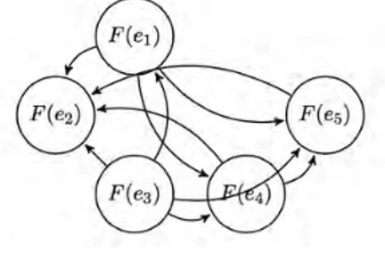
Let Mr. X priorities are ranked as beautiful, in green surrounding, cheap, expensive and wooden houses. According to this priority ranking, we can define a soft set relation on ( ,F E) as follows:
( , ) G V E 1( ,1 1) G V E G 1 and 1 , V V E E 1 E V1. V , V Kn,
,
,
,
a b V a
b
G , G G,3 1 3 4 3 5 3 2 1 4 1 5 1 2 4 5 4 2 5 2 { ( ) ( ), ( ) ( ), ( ) ( ), ( ) ( ), ( ) ( ), ( ) ( ), ( ) ( ), ( ) ( ), ( ) ( ), ( ) ( )}. R F e F e F e F e F e F e F e F e F e F e F e F e F e F e F e F e F e F e F e F e
And the graph representation of Ris as follows:
Graph 2. Graph representation of soft set relationR.
Step 1: Count the incoming and outgoing paths to each vertex and represent them with ordered pairs where first component is the number of incoming ways, while second component is the number of outgoing ways.
For the node F e( )1 in Example 3.6, we have 1 incoming and 3 outgoing ways. Thus, we get the pair
(1, 3) for the nodeF e( )1 . In this example, all ways are listed below:
1 2 3 4 5 ( ) (1,3) ( ) (4, 0) ( ) (0, 4) ( ) (2, 2) ( ) (3,1) F e F e F e F e F e
Step 2: Examine the images of each F e( i) to
determine the existence of the elements of universal set. For this purpose, we will see the images F e( )i as
vectors and each of its element represents the existence of elements of universal set in same order. After applying the method to Example 3.6, the existence vectors are as follows:
1 2 3 2 2 3 5 3 1 4 4 1 5 1 2 (0,1,1, 0, 0, 0) for ( ) { , } (0,1,1, 0,1, 0) for ( ) { , , } (1, 0, 0,1, 0, 0) for ( ) { , } (1, 0, 0, 0, 0, 0) for ( ) { } (1,1, 0, 0, 0,1) for ( ) { , , F e h h F e h h h F e h h F e h F e h h h6} Step 3: Find the incoming and outgoing values for eachF e( )i . One can find these values by adding the numbers of incoming and outgoing ways of F e( i) to
each component of vectors. Incoming and outgoing values are evaluated below for Example 3.6. First
vectors represent incoming values while the second represent outgoing values for h h h h h1, 2, 3, 4, 5 and h6 in
1 ( ) F e , F e( 2), F e( 3), F e( 4), and F e( 5) respectively: 1 2 3 4 5 ( ) (0, 2, 2, 0, 0, 0) (0, 4, 4, 0, 0, 0) ( ) (0, 5, 5, 0, 5, 0) (0,1,1, 0,1, 0) ( ) (1, 0, 0,1, 0, 0) (5, 0, 0, 5, 0, 0) ( ) (3, 0, 0, 0, 0, 0) (3, 0, 0, 0, 0, 0) ( ) (4, 4, 0, 0, 0, 4) (2, 2, 0, 0, 0, 2) F e F e F e F e F e
Step 4: Compute the total incoming and outgoing values for each hi. The Maximum incoming value provides us the choice. If there are more than one objects that have maximal incoming value, then the maximum outgoing value of the objects that have maximal incoming values will give us the choice.
Total incoming and outgoing values for 1, 2, 3, 4, 5
h h h h h and h6 are
(8,10), (11,7), (7,5), (1,5), (5,1) and (4,2), respectively. Hence the house will be h2 according to our algorithm.
The previous results that we have obtained in the stated steps can be summarized in Table 1, where vertices of graph are given in the first column while the elements of universal set are in the first row. Entries in the table show the existence, the change and the total values for each hi in the setsF e( )i . Left
subscript of F e( )i symbolizes the number of
incoming ways while the right subscript symbolizes the number of outgoing ways. We can also use both subscripts of the entries to represent the effects of incoming and outgoing ways to each element of universal set which were found in Step 3.
Table 1. Summarized Algorithm for Example 3.6.
1 h h2 h3 h4 h5 h6 1F e( )1 3 000 214 214 000 000 000 4F e( 2)0 000 5 11 5 11 000 5 11 000 0F e( 3)4 5 11 000 000 5 11 000 000 2F e( 4)2 313 000 000 000 000 000 3F e( 5 1) 412 412 000 000 000 412 (8,10) (11,7) (7,5) (1,5) (5,1) (4,2)
Example 3.7. Let Ube the set of cars under consideration, U { ,c c1 2,c3,c4,c5,c6,c7} and let E be the parameter set such that:
1 2 3
4 5 7
8
{ diesel, gasoline, light color, dark color, manuel, new,
second hand}. E e e e e e e e
Let a soft set (F A, ) describes the attractiveness of the cars that Mr. X is going to buy. Consider
1 2 3
4 5 7 8
A={e =diesel, e =gasoline, e =light color,
e =dark color,e =manuel, e =new, e =second hand} and 1 1 3 5 2 2 4 6 7 3 1 3 4 4 1 7 5 5 6 7 7 1 2 7 8 3 4 5 6 ( ) { , , }, ( ) { , , , }, ( ) { , , }, ( ) { , }, ( ) { , , }, ( ) { , , }, ( ) { , , , }. F e c c c F e c c c c F e c c c F e c c F e c c c F e c c c F e c c c c
Let Mr. X has priority ranking in getting manual, diesel, new, second hand and light color cars. According to this priority, we can define a soft set relation on ( ,F E) as follows: 1 5 7 5 8 5 3 5 7 1 8 1 3 1 8 7 3 7 3 8
{ ( )
( ), ( )
( ), ( )
( ),
( )
( ), ( )
( ), ( )
( ), ( )
( ), ( )
( ), ( )
( ), ( )
( )}.
R
F e
F e F e
F e F e
F e
F e
F e F e
F e F e
F e F e
F e F e
F e F e
F e F e
F e
Graph of this relation
R
is given in Graph 3.Graph 3. Graph representation of relation
R
.Let’s apply the above method to this problem. Step 1: Counting paths for each node:
1 3 5 7 8 ( ) (3,1) ( ) (0, 4) ( ) (4, 0) ( ) (2, 2) ( ) (1,3) F e F e F e F e F e
Step 2: Images ofF e( )i s and the existence vectors:
1 1 3 5 3 2 3 4 5 5 6 7 7 1 2 7 8 3 4 5 6 ( ) { , , } (1, 0,1, 0,1, 0, 0) ( ) { , , } (0,1,1,1, 0, 0, 0) ( ) { , , } (0, 0, 0, 0,1,1,1) ( ) { , , } (1,1, 0, 0, 0, 0,1) ( ) { , , , } (0, 0,1,1,1,1, 0) F e c c c F e c c c F e c c c F e c c c F e c c c c
Step 3: Change of images:
1 3 5 7 8 ( ) (4, 0, 4, 0, 4, 0, 0) (2, 0, 2, 0, 2, 0, 0) ( ) (0,1,1,1, 0, 0, 0) (0, 5, 5,5, 0, 0, 0) ( ) (0, 0, 0, 0,5, 5, 5) (0, 0, 0, 0,5, 5, 5) ( ) (3, 3, 0, 0, 0, 0, 3) (3, 3, 0, 0, 0, 0, 3) ( ) (0, 0, 2, 2, 2, 2, 0) (0, 0, 4, 4, 4, 4, 0) F e F e F e F e F e
Step 4: Total incoming and outgoing values 1, , , , , 2 3 4 5 6 and 7
c c c c c c c are (7,5), (4,8), (7,11), (3,9), (11,7), (7,5) and (8,4), respectively. Hence the car will be c5according to our algorithm.
Same results obtained in the above steps are summarized in Table 2.
Table 2. Summarized Algorithm for Example 3.7.
1 c c2 c3 c4 c5 c6 c7 3F e( )1 1 412 000 412 000 412 000 000 0F e( 2)4 000 1 51 1 51 1 51 000 000 000 4F e( 5)0 000 000 000 000 5 11 5 11 5 11 2F e( 7)2 313 313 000 000 000 000 313 1F e( 8)3 000 000 1 41 1 41 1 41 1 41 000 (7,5) (4,8) (7,11) (3,9) (11,7) (7,5) (8,4)
The following example is about Information Systems (IS) that was given by Jiang, et. al. (2011). We have successfully applied our designed Decision Making method to this example.
Example 3.8: Suppose that there are six papers
1, 2, 3, 4, 5, 6
p p p p p p in IS (Table 3) and four keywords a a1, 2,a a3, 4 stand for “keyword 1= Semantic web”, “keyword 2”=Description logics”, “keyword 3=Web Ontology Language”, and “keyword 4=Reasoning Rule”, respectively.
Table 3. Information system (IS).
U a1 a2 a3 a4
1
p DLs Soft Sets Ontology Decision
Making 2 p Data mining Data bases Machine learning Rule 3
p Ontology Rule DLs OWL
4
p OWL Ontology KR DLs
5
p LP ASP First Order
Logic Prolog
6
p ASP Prolog LP KR
Assume that Mr. X wants to obtain a closely related research paper in the area of “Semantic web” using the following query:
“Keyword 1”=Semantic web, “keyword 2”=Description logics, “keyword 3”=Web Ontology Language, and “keyword 4” =Reasoning Rule.
It is reported Jiang, et. al. (2011) that the approximately resultant soft set, where {a a1, 2,a3,a4}
is the parameter set and {p1,p2,p3,p4,p5,p6} is the universal set, is obtained from certain semantic relations between the information system and the query as follows: 1 1 3 4 5 6 2 3 4 5 3 1 3 4 5 6 4 2 3 4 6 ( ) { , , , , }, ( ) { , , }, ( ) { , , , , }, ( ) { , , , } F a p p p p p F a p p p F a p p p p p F a p p p p .
Now, let’s find the choice object for Mr. X using our Decision Making method.
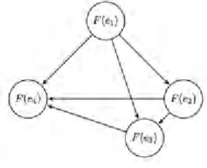
A soft set relation R can be obtained by given query as: 1 2 1 3 1 4 2 3 2 4 3 4 { ( ) ( ), ( ) ( ), ( ) ( ), ( ) ( ), ( ) ( ), ( ) ( )}. R F a F a F a F a F a F a F a F a F a F a F a F a
Hence, the graph representation of Ris:
Graph 4. Graph representation of relationR.
After applying our Decision Making method to this example, we obtain the choice objects as p3 andp4 (Table 4). These choice objects are the same as stated by Jiang, et. al. (2011).
Table 4. Summarized Algorithm for Example 3.8.
1 p p2 p3 p4 p5 p6 0F e( )1 3 1 41 000 1 41 1 41 1 41 1 41 1F e( 2)2 000 000 213 213 213 000 2F e( 3)1 312 0
0
0 312 312 312 312 3F e( 4)3 000 414 414 414 000 414 (4,6) (4,4) (10,13) (10,13) (6,9) (8,10) 4 CONCLUSIONSIN this study, we have designed a Decision Making Method by using graph representation of soft set relations that is a new perspective for the soft set relations. By utilizing this method, complex social life
problems in different areas can be solved effectively. This method can be also used in various decision making methods including artificial intelligence.
5 ACKNOWLEDGEMENTS
THE authors deeply thank to editor and referees for their valuable comments and special thanks to Said Nadeem, (Assistant Professor, Muğla Sıtkı Koçman University) for grammatical corrections.
6 REFERENCES
Acar, U., Koyuncu, F., & Tanay B. (2010). Soft sets and soft rings. Computer & Mathematics with Applications, 59, 3458–3463
Aktaş, H. & Çağman, (2007). N. Soft sets and soft groups. Information Sciences, 117, 2726-2735. Babitha, K.V. & Sunil, J.J. (2010). Soft set relations
and functions, Computer & Mathematics with Applications, 60, 1840-1849.
Babitha, K.V. & Sunil, J.J. (2011). Transitive closures and ordering on soft sets. Computer & Mathematics with Applications, 62, 2235-2239. Ballı, S. & Turker, M. (2017). A Fuzzy Multi-Criteria
Decision Analysis Approach for the Evaluation of the Network Service Providers in Turkey. Intelligent Automation & Soft Computing, 1-7. Çağman, N. & Enginoğlu, S. (2010). Soft matrix
theory and its decision making. Computer & Mathematics with Applications, 59, 3308-3314. Dauda, M.K., Aliyu I., & Ibrahim A. M. (2013).
Partial Ordering in Soft Set Context. Mathematical Theory and Modeling, 3, No.8.
Grimaldi, R. P. (2004) Discrete and Combinatorial Mathematics (an Applied Introduction), United States of America, Addison-Wesley, Fifth Edition. Gunduz, C. & Bayramov, S. (2011a). Fuzzy soft
modules. International Mathematical Forum, 6, No.11, 517-527.
Gunduz, (Aras) C. & Bayramov, S. (2011b). Intuitionistic fuzzy soft modules. Computer & Mathematics with Applications, 62, 2480-2486. Ibrahim, A.M., Dauda, M.K., & Singh, D. (2012).
Composition of soft set relations and construction of transitive closure. Mathematical Theory and Modeling, 2 No.7.
Jiang, Y., Liu, H., Tang, Y., & Chen Q. (2011). Semantic decision making using ontology-based soft sets, Mathematical and Computer Modelling, 53, 1140-1149.
Maji, P.K., Biswas, R., & Roy, A.R. (2003). Soft set theory. Computers and Mathematics with Applications, 45, 555-562.
Molodtsov, D. (1999). Soft Set Theory-First Result. Computers and Mathematics with Applications, 37, 19-31.
Ozturk, T.Y., Gunduz, C.A., & Bayramov S. (2013). Inverse and direct systems of soft modules. Annals
of Fuzzy Mathematics and Informatics, 5, No.1, 73-85.
Park, J.H., Kim, O.H., & Kwun, Y.C. (2012). Some properties of equivalence soft set relations. Computers & Mathematics with Applications 63, 6, 1079-1088.
Tanay, B. & Yaylalı, G. (2015). A Method for Decision Making by Using Soft Intervals. International Conference on Recent Advances in Pure and Applied Mathematics (Icrapam).
Wang, C. & Wang, J. (2016). A multi-criteria decision-making method based on triangular intuitionistic fuzzy preference information. Intelligent Automation & Soft Computing, 22:3, 473-482.
Yang, H. & Guo, Z. (2011). Kernels and closures of soft set relations and soft set relation mappings. Computers and Mathematics with Applications, 61, 651-662.
Zeinalova, L.M. (2014). Expected Utility Based Decision Making Under Z-Information. Intelligent Automation & Soft Computing, 20:3, 420-431. Zhang, X. (2014). On Interval Soft Sets with
Applications. International Journal of Computational Intelligence Systems, 7:1, 186-196.
7 NOTES ON CONTRIBUTORS
Nazan ÇAKMAK POLAT is a Research Assistant for Department of Mathematics. Her major is Topology, Soft Set theory and Algebra.
Gözde YAYLALI is Research Assistant for Department of Mathematics. Her major is Topology, Soft Set Theory and Fuzzy Set Theory. Email: [email protected]
Bekir TANAY is a Associated Professor at Muğla Sıtkı Koçman University. His main research interests include Topology, Algebraic Topology, Soft Set theory and Fuzzy Set Theory.