SLIM: Scalable Linkage of Mobility Data
Fuat Basık
∗[email protected]
Amazon Web Services
Hakan Ferhatosmanoğlu
[email protected]
University of Warwick
Buğra Gedik
[email protected]
Bilkent University
ABSTRACT
We present a scalable solution to link entities across mobility datasets using their spatio-temporal information. This is a fundamental problem in many applications such as linking user identities for security, understanding privacy limitations of location based services, or producing a unified dataset from multiple sources for urban planning. Such integrated datasets are also essential for service providers to optimise their services and improve business intelligence. In this paper, we first propose a mobility based representation and similar-ity computation for entities. An efficient matching process is then developed to identify the final linked pairs, with an automated mechanism to decide when to stop the linkage. We scale the process with a locality-sensitive hashing (LSH) based approach that significantly reduces candidate pairs for matching. To realize the effectiveness and efficiency of our techniques in practice, we introduce an algorithm called SLIM. In the experimental evaluation, SLIM outperforms the two existing state-of-the-art approaches in terms of preci-sion and recall. Moreover, the LSH-based approach brings two to four orders of magnitude speedup.
KEYWORDS
mobility data; data integration; scalability; entity linkage
ACM Reference Format:
Fuat Basık, Hakan Ferhatosmanoğlu, and Buğra Gedik. 2020. SLIM: Scalable Linkage of Mobility Data. In Proceedings of the 2020 ACM SIGMOD International Conference on Management of Data (SIG-MOD’20), June 14–19, 2020, Portland, OR, USA. ACM, New York, NY, USA, 16 pages. https://doi.org/10.1145/3318464.3389761
∗Work done prior to author’s employment with Amazon. This work is
included in the author’s PhD thesis.
Permission to make digital or hard copies of all or part of this work for personal or classroom use is granted without fee provided that copies are not made or distributed for profit or commercial advantage and that copies bear this notice and the full citation on the first page. Copyrights for components of this work owned by others than ACM must be honored. Abstracting with credit is permitted. To copy otherwise, or republish, to post on servers or to redistribute to lists, requires prior specific permission and/or a fee. Request permissions from [email protected].
SIGMOD’20, June 14–19, 2020, Portland, OR, USA © 2020 Association for Computing Machinery. ACM ISBN 978-1-4503-6735-6/20/06. . . $15.00 https://doi.org/10.1145/3318464.3389761
1
INTRODUCTION
With the proliferation of smart phones integrated with posi-tioning systems and the increasing penetration of Internet-of-Things (IoT), mobility data has become widely available [10]. A vast variety of mobile services and applications have a location-based context and produce spatio-temporal records. For example, most payments produce records containing the time of the payment and the location of the store. Lo-cation sharing services such as Swarm help people share their whereabouts. These records contain information about both the entities and the environment they were produced in. Availability of such data supports smart services in areas including healthcare [29], computational social sciences [28], and location-based marketing [48].
There are many studies that analyze location based data for social good, such as reducing traffic congestion, lower-ing air pollution levels, analyzlower-ing the spread of contagious diseases, and modelling of the pandemic virus spreading process [8, 11, 12]. Most of the studies focus on a single dataset, which provides only a partial and biased state, fail-ing to capture the complete patterns of mobility. To produce a comprehensive view of mobility, one needs to integrate multiple datasets, potentially from disparate sources. Such integration enables knowledge extraction that cannot be ob-tained from a single data source, and benefits a wide range of applications and machine learning tasks [34, 49]. Exam-ples include discovering regional poverty by jointly using mobile and satellite data where accurate demographic in-formation is not available [39], and measuring urban social diversity by jointly modeling the attributes from Twitter and Foursquare [15].
Spatio-temporal linkage is necessary to avoid over- or under-estimation of population densities using multiple sources of data, e.g., signals from wifi based positioning and mobile applications. It is also essential in user identi-fication for security purposes, and understanding privacy consequences of anonymized mobility data [44]. An outcome of work such as ours is to help developing privacy advisor tools where location based activities are assessed in terms of their user identity linkage likelihood.
Identifying the matching entities across mobility datasets is a non-trivial task, since some datasets are anonymized due to privacy or business concerns, and hence unique identifiers are often missing. Since spatio-temporal information is the only feature guaranteed to exist in all mobility datasets, our
approach decreases the number of features the linkage de-pends on, and can be used for other applications. This helps avoid the use of personally identifying information (PII) [32] and additional sensitive data, and simplifies the procedures to share data for social good and research purposes without having to explicitly expose PII. It enables use and collection of minimal data, which is a requirement in major privacy and data protection regulations, such as GDPR. As such, in this paper, we present a scalable solution to link entities across mobility datasets, using only their spatio-temporal information. There are several challenges associated with such linkage across mobility datasets.
First, a summary representation for the spatio-temporal records and an associated similarity measure should be de-veloped. The similarity score should capture the closeness, in time and location, of the records. Yet, unlike the traditional measures, it should not penalize the absence of records in one dataset for a particular time window, when the other dataset has records for the same time window. This is because different services are typically not used synchronously.
Second, once similarity scores are assigned to entity pairs, an efficient matching process needs to identify the final linked pairs. A challenging problem is to automate the de-cision to stop the linkage to avoid false positive links. In a real-world setting, it is unlikely to have the entities from one dataset as a subset of the other, which is a commonly made assumption. This is an important but so far overseen issue in the literature [4, 43, 47].
Third, efficiency and scalability of the linkage process are essential, given the scale and dynamic nature of location datasets. Even a static comparison of each pair of entities would require quadratic number of similarity computations over millions of entities. Avoiding exhaustive search and focusing on a small amount of pairs that are likely to be matching can scale the linkage to a larger number of entities for real-life dynamic cases.
In this work, we present a scalable linkage solution, SLIM, for efficiently finding the matching entities across mobility datasets, relying only on the spatio-temporal information.
Given an entity, we introduce a mobility history repre-sentation, by distributing the recorded locations over time-location bins (Sec. 2) and defining a novel similarity score for histories, based on a scaled aggregation of the proximities of their matching bins (Sec. 3.1). The proposed similarity defi-nition provides several important properties. It awards the matching of close time-location bins and incorporates the frequency of the bins in the award amount. It normalizes the similarity scores based on the size of the histories in terms of the number of time-location bins. Moreover, while it does not penalize the score when one entity has activity in a par-ticular time window but the other does not, it does penalize the existence of cross-dataset activities that are close in time
but distant in space (aka alibis [2, 3]). This is an essential property that supports mobility linkage.
The similarity scores are used as weights to construct a bipartite graph which is used for maximum sum matching. The matched entities are linked via an automated linkage thresholding (Sec. 3.2). We first fit a mixture model, e.g., Gaussian Mixture Model (GMM), with two components over the distribution of the edge weights selected by the maximum sum bipartite matching. One of these components aims to model the true positive links and the other one is for false positive links. We then formulate the expected precision, recall, andF 1-score for a given threshold, based on the fitted model. This is used to automatically select the threshold that provides the maximumF 1-Score and use it to filter the results to produce the linkage.
To address the scalability challenge, we develop a Locality Sensitive Hashing (LSH) [16] based approach using the con-cept of dominating grid cell (Sec. 4). Dominating grid cells contain most records of the owner entity during a given time period. We construct a list of dominating cells to act as signatures and then apply a banding technique, by dividing the signatures intob bands consisting of r rows, where each band is hashed to a large number of buckets. The goal is enable signatures such that entities with similarity higher than a thresholdt are hashed to the same bucket at least once. Our experimental evaluation (Sec. 5) shows that this LSH based approach brings two to four orders of magnitude speedup to linkage with a slight reduction in the recall.
In summary, this work makes the following contributions: • Model. We devise a hierarchical summary representation for mobility records of entities along with a novel method to compute their similarity. The similarity score we introduce does not only capture the closeness in time and location, but also tolerates temporal asynchrony and penalizes the alibi records, which are essential contributions for mobility linkage.
• Algorithm. We develop the SLIM algorithm for linking enti-ties across mobility datasets. It relies on maximum bipartite matching over a graph formed using the similarity scores. We provide an automated mechanism to detect an appropri-ate threshold to stop the linkage; a crucial step for avoiding false positives.
• Scalability. To scale linkage to large datasets, we develop an LSH based approach which brings a significant speedup. To our knowledge, this is the first application of LSH in the context of mobility linkage.
• Evaluation. We perform extensive experimental evaluation using real-world datasets, compare SLIM with two existing approaches (STLink [3], GM [43]), and show superior per-formance in terms of accuracy and scalability.
2
PRELIMINARIES
In this section, we first present the notation used throughout the paper. We then formally define the linkage problem, and describe how mobility histories are represented.
2.1
Notation
Location Datasets. A location dataset is defined as a collec-tion of usage records from a locacollec-tion-based service. We use I and E to denote the two location datasets from the two services, across which the linkage will be performed. Entities. Entities are real-world systems or users, whose usage records are stored in the location datasets. They are represented in the datasets with their ids. An id uniquely identifies an entity within a dataset. However, since ids are anonymized, they can be different across different datasets and cannot be used for linkage. The set of all entities of a location dataset is represented asUE, where the subscript
represents the dataset. Throughout this work, we useu ∈ UE
andv ∈ UI to represent two entities from the two datasets.
Records. Records are generated as a result of entities inter-acting with the location-based service. Each record is a triple {u,l,t }, where for a record r ∈ E, r .u represents the id of the entity associated with the record. Similarly,r .l and r .t repre-sent the location and timestamp of the record, respectively. We assume that the record locations are given as points. Our approach can be extended to datasets that contain record locations as regions, by copying a record into multiple cells within the mobility histories using weights.
2.2
Problem Definition
With these definitions at hand, we can define the problem as follows. Given two location datasets, I and E, the problem is to find a one-to-one mapping from a subset of the entities in the first set to a subset of the entities in the second set. This can be more symmetrically represented as a function that takes a pair of entities, one from the first dataset and a second from the other, and returns a Boolean result that either indicates a positive linkage (true) or no-linkage (false), with the additional constraint that an entity cannot be linked to more than one entity from the other dataset. A positive linkage indicates that the relevant entities from the two datasets refer to the same entity in real-life.
More formally, we are looking for a linkage function M : UE×UI → {0, 1}, with the following constraint:
∃ u,v s.t. M(u,v) = 1
⇒∀u′, u, v′, v, M(u′,v) = M(u,v′)= 0 Note that the size of the overlap between sets of entities from different services may not be known in advance. Even when it is known, finding all positive linkages is often not
[t 0 t 1, ) . . . . . . [t 0 t 2, ) [t 2 t 4, ) [t n− 2 t n, ) [t 1 t 2, ) [t 2 t 3, ) [t n− 2 t n− 1, )[t n− 1 t n, ) . . . .. . [t 0 t n/2, ) [t n/2 t n, ) [t 0 t n, ] [t 3 t 4, ) Legend Set of Grid Cell Ids Cell Id to Count Mapping
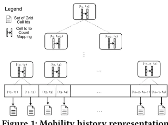
Figure 1: Mobility history representation possible, as some of the entities may not have enough records to establish linkage.
2.3
Mobility Histories
We organize the records in a location dataset into mobility histories. Given an entity, its mobility history consists of an aggregated collection of its records from the dataset. Repre-sentation of the mobility history should be generic enough to capture the differences and spatio-temporal heterogeneity of the datasets. To address this need, we propose a hierarchical representation for mobility histories, which distributes the records over time-location bins.
In the temporal domain, the data is split into time windows which are hierarchically organized as a tree to enable efficient computation of aggregate statistics. The leaves of this tree hold a set of spatial cell ids. A cell id is present at a leaf node if the entity has at least one record whose spatial location is in that cell and the record timestamp is in the temporal range of the window. Each non-leaf node keeps the occurrence counts of the cell ids in its sub-tree. The space complexity of this tree is similar to a segment tree, O(|E | + |I|). As we will detail in Sec. 4, the information kept in the non-leaf nodes is used for scalable linkage. The cells are part of spatial partitioning of locations. For this, we use S21, which divides the Earth’s surface into 31 levels of hierarchical cells, where, at the smallest granularity, the leaf cells cover 1cm2.
We deliberately form the mobility history tree via hierar-chical temporal partitioning, and not via hierarhierar-chical spatial partitioning. This is because spatial partitioning is not ef-fective in detecting negative linkage (alibi [3]). Given two locations in the same temporal window, if it is not possible for an entity to move from one of these locations to the other within the width of the window, then these two records are considered as a negative link, i.e., alibi. To calculate the sim-ilarity score of an entity pair, we compare their records to those that are in close temporal proximity. Record pairs that are close in both time and space are awarded, whereas record pairs that are close in time but distant in space are penalized.
Hence, we favor fast retrieval of records based on temporal information over based on spatial information.
Both the temporal window size used for the leaf nodes and the S2 level (spatial granularity) used for the cells are configurable. As detailed later, we auto-tune the spatial gran-ularity for a given temporal window size using the trade-off between accuracy and performance of the linkage.
2.4
Overview of the Linkage Process
Figure 1 shows an example mobility history of an entity. Each leaf keeps a set of locations, represented with cell ids. Each non-leaf node keeps the information on how many times a cell id has occurred at the leaf level in its sub-tree.
The linkage is performed in three steps. First, a Locality-Sensitive Hashing based filtering step reduces the number of entity pairs that needs to be considered for linkage. The sec-ond step computes the pairwise similarity scores of entities from the two datasets. The similarity scores are computed based on a formula that determines how similar the mobility histories are. The computed similarities are used as weights to construct a bipartite graph of the entities from the two datasets. The final step is to apply a maximum sum bipar-tite matching, where the matched entities are considered as linked. Once the matches are found, they are output as link-age only if their scores are above the stop similarity threshold, which is automatically identified.
3
MOBILITY HISTORY LINKAGE
In this section we describe the computation of similarity scores of mobility history pairs and the maximum weight bipartite matching for linkage. Since the set of entities in the two location datasets are not necessarily identical and the amount of intersection between them is not known in advance, we also discuss how to find an appropriate score threshold to limit the number of entities linked.
3.1
Mobility History Similarity Score
The similarity score of a pair of mobility histories should capture closeness in time and location. This score should not require a consistent matching of time-location bins across two histories. This is because the mobility histories are not synchronous, i.e., a record is not necessarily present for the same timestamp in both of the datasets. Therefore, the simi-larity score needs to aggregate the proximities of the time-location bins, different from the traditional techniques where similarity measures are defined over records, like Minkowski distance or Jaccard similarity. We define a number of desired properties for the similarity score:
1) Award the matching of close time-location bins. While the similarity score contribution of exactly matching time-location bins is obvious, one should also consider bins that
are from the same temporal window but are from different yet spatially close cells. Such time-location bins are deemed close and they should contribute to the similarity score rela-tive to their closeness.
2) Tolerate temporal asynchrony, that is, do not penalize the similarity when one entity has records in a particular time window but the other does not. This case is common when the location datasets are obtained from asynchronous services. While spatio-temporally close usage should con-tribute to the similarity, lack of it for a particular time window should not penalize the score.
3) Penalize alibi time-location bins. Time-location bins that are from the same time window but whose cells are so distant in space that it is not possible for an entity to move between these cells within the time window are considered as alibi bins. They are counter evidences in terms of linking the entities and penalized in the similarity score.
4) Award infrequent cells in matching time-location bins. While summing up the proximities of the matched time-location bins, the uniqueness of the cells should be awarded as they are stronger indicators of similarity than cells that are seen frequently.
5) Normalize the similarity score contributions based on the size of the mobility histories in terms of the number of time-location bins. If not handled properly, the skew in the number of time-location bins would result in the mobil-ity histories with too many bins to dominate the similarmobil-ity scores over the shorter ones.
3.1.1 Proximity of Time-Location Bins. One of the desired properties of the time-location bin proximity was tolerating temporal asynchrony. Hence, we consider only the tempo-rally close time-location bins in our proximity computation. Let T be a binary function that takes the value of 1 if the two given time-location bins are associated with the same temporal window and 0 otherwise. Lete = {w,c} and i = {w,c} be two time-location bins where e.w and i.w are two temporal windows ande.c and i.c are two spatial grid cells. We define T formally as T (e,i) = [e.w = i.w].
We define the spatial proximity of a pair of time-location bins as an inverse function of the geographical distance of their locations. However, we use an upper bound on the geographical distance to capture the concept of alibis. This upper bound, referred to as the runaway distance, is defined as the maximum distance an entity can travel within the given temporal window. It is represented as R and calculated by multiplying the width of the temporal window with the maximum speed,α, at which an entity can travel. Let w be a temporal window and |w | be the width of it, then R = |w| ·α. In practice, the value ofα could be defined using a dataset-specific speed limit. We define the proximity function P
formally as follows:
P(e,i) = T (e,i) · log2(2 −min(d(e.c, i.c)/R, 2)) (1) whered is a function that calculates the minimum geograph-ical distance between two grid cells.
When a given pair of time-location bins are not from the same temporal window, the outcome of this function becomes 0. When they are from the same temporal window and the same spatial cell, the outcome becomes 1 — the highest value it can take. As the distance increases up to the runawayR, the value goes down to 0 with an increasing slope. If the distance is more thanR, the outcome becomes negative, reaching −∞ as the distance reaches two times the runaway distance. This is a simple yet effective technique to capture the alibi record pairs. In a real-world setting, the location data might be inaccurate. Therefore, while the decrease to negative values is steep, it is still a continuous function that allows a small number of alibi record pairs whose distance from each other is slightly larger than the runaway distance.
The proximity function P is designed so that our similarity score satisfies the first three of the required properties we have outlined earlier, namely: awarding the matching of close time-location bins, tolerating temporal asynchrony, and penalizing the alibis.
3.1.2 Aggregation of Proximities. The similarity computa-tion is performed over the time-locacomputa-tion bins at the leaves of the histories. For entityu ∈ UE (andv ∈ UI), we
repre-sent the set of time-locations bins asHu (andHv), where e ∈ Hu = {c,w} (and i ∈ Hv = {c,w}) represents a
time-location bin with the time windoww and the grid cell c. Given a pair of mobility histories, the computation starts with constructing pairs of time-location bins whose proxim-ity will be computed and included in the aggregation.
The design of mobility history trees blocks the records by distributing them over time-location bins. This is similar to sorted neighborhood based blocking of traditional record linkage algorithms [7]. Normally, pairs of time-location bins would have been constructed using Cartesian product over events from the same temporal window. However, this would be over-counting, as a time-location bin will end up partic-ipating in multiple pairs. Therefore, we first introduce a pairing function N (u,v), which computes the set of time-location bin pairs to be included in the aggregation for a pair (u,v) of mobility histories. Later, in the experimental evaluation, we show that this pairing functionN is more accurate compared to all pairs matching.
We restrict ourselves to time-location bin pairs from corresponding time windows, as this guarantees that the pairs satisfy the temporal proximity, T . As such, we have N (u,v) = ÐwNw(u,v). Given a time window w, we com-pute Nw(u,v) by first selecting the time-location bin pair
(e, i) with e.w = i.w = w that has the smallest geographi-cal distanced(e.c, i.c). Once this pair is added into Nw(u,v),
pairs containing any one of the selected time-location bins, that ise or i, are removed from the remaining set of candi-date pairs. We repeat these two operations until there are no time-location bins left in the smaller mobility history.
Once the set of time-location bin pairs to include in the aggregation are found, we define the similarity score function of two mobility histories for the entitiesu ∈ UEandv ∈ UI,
as follows:
S(u,v) = Í
{e,i }∈N(u,v)P(e,i)
min (idf (e, E),idf (i, I)) L(u, E)L(v, I)
where: L(u,E) = (1 − b) + bÍ |Hu|
u′∈UE|Hu′|/ |UE| (2)
The similarity function, S, has three main components. The first component is the proximity P, as defined in Eq. 1. For the time-location bin pairs identified by the pairing func-tion N , we sum up the proximities. The other two compo-nents deal with the scaling of the proximity value, in order toi) normalize the differences in the mobility history sizes in terms of the bin counts, andii) award infrequent cells in the matching. These two properties implement the last two desired properties from Sec. 3.1.
Histories with a higher number of time-location bins, compared to other histories from the same location dataset, would be more likely to be similar with the histories from the opposite dataset. We introduce a normalization function L, for both histories, which makes the contribution of each bin pair to the similarity score inversely proportional with the relative sizes of the histories. The relative size of a mobility history is defined as the ratio of the number of time-location bins it contains over the average number of time-location bins from the same dataset.
In order to tune the impact of the mobility history size in terms of time-location bins, we add a parameterb, which takes a value between 0 and 1. At one extreme,b = 0, the de-nominator becomes 1, i.e., the history lengths are ignored. At the other end,b = 1, the denominator becomes the product of the relative history sizes. This is inspired by BM25 [33] — a ranking function used in document retrieval, which avoids bias towards long documents.
The final component of the similarity function is the idf multiplier. This component is analogous to inverse document frequency in information retrieval. It awards uniqueness of a pair of location bins. If an entity is in an infrequent time-location bin, i.e., the number of other entities from the same dataset in the same time-location bin is low, the contribution of this bin to the similarity score should be higher. Likewise, if a time-location bin is highly common among entities of one dataset, the contribution should be lower. As the frequency of time-location bins might differ across datasets, we take
Alg. 1: SLIM: Scalable Linkage of Mobility Histories
Data: E, I: Location datasets to be linked Result: L: Linked pairs of entities
{HE, HI} ←CreateHistories(E, I) ▷ Histories from datasets E ← {} , V ← {} ▷ Initialize edges and vertices forHu ∈ HEdo ▷ For each history in first history set
WHu ←Hu.дetAllW indows() ▷ Get all windows of Hu forHv∈LSHFilterPairs(u) do ▷ For a candidate history
S ← 0 ▷ Initialize similarity score
WHv ←Hv.дetAllW indows() ▷ Get all windows of Hv forw ∈ WHu ∩WHv do ▷ For a common window N ← Nw(u,v) ▷ Mutually nearest pairs S ← S + S(N ) ▷ Update similarity (see Eq. 22)
N′← N′w(u,v) ▷ Mutually furthest pairs
for (e, i) ∈ N′do ▷ For each mutually furthest pair
D ← S({(e, i)}) ▷ Delta similarity ifD < 0 then ▷ If an alibi is detected S ← S + D ▷ Update similarity ifS > 0 then ▷ If score is positive
V ← V ∪ {u,v} ▷ Add to vertex set
E ← E ∪ {(u,v; S)} ▷ Add to weighted edge set return L ←LinkPairs(E,V ) ▷ Return linked entity pairs
the idf score that makes the lowest contribution.id f of a time-location bin equals to the logarithm of the ratio of the number of mobility histories to the number of mobility histories that contain the given time location bin. Formally, given a time location bin,e ∈ Hu, for the entityu ∈ UE, we
calculateid f (e, E) as follows:
id f (e, E) = log (|UE|/|{u ∈ UE |e ∈ Hu}|) (3)
Algorithm 1, SLIM, shows the linkage of the mobility his-tories using our similarity score. SLIM starts by creating the mobility histories from the location datasets. It then finds the mutually nearest neighbor (MNN) pairs for each correspond-ing time window (N ). The similarity score is computed by aggregating the weighted proximities for these pairs, as it was outlined in Eq. 2.
An additional step that uses mutually furthest neighbors (MFN) further improves the effectiveness of alibi detection. We illustrate this with an example. Given a temporal window, lete1be an entity with a single time-location binb1ande2
be an entity with two such bins,b2 andb3. Assume that
the distance betweenb1andb2isd units and the distance
betweenb1andb3isd + r units, where d < r and r is the
runaway distance. While MNN would return the pair with distanced (missing the alibi), MFN would help us capture the alibi time-location bin pair. This is shown in the algorithm with the inner-most for loop, where N′(MFN) function acts
similar to N (MNN), but it chooses the pairs with the furthest
2We overload the notation such that S takes the bin pairs as input.
distance. To avoid double counting, we only consider these pairs if they are alibis.
Once the similarity scores are computed for the mobility history pairs, they are used to construct a weighted bipartite graph. If the score is negative, no edges are added to the graph. Next, we describe how to perform maximum sum bipartite matching and decide a stop point for the linkage.
3.2
Final Linkage
The SLIM algorithm computes a weighted bipartite graph G(E,V ), where V = UE∪UI andE is the set of edges
be-tween them. This bipartite graph is used to find a maximum weighted matching where the two ends of the selected edges are considered linked. To avoid ambiguity in the results, the selected edges should not share a vertex. Since the matching is performed on a bipartite graph, there is no edge between two entities from the same dataset.
Finding this matching is a combinatorial optimization problem known as the assignment problem, with many opti-mal and approximate solutions [21, 22]. We adapt a simple greedy heuristic, which links the pair with the highest simi-larity at each step. Maximum weighted matching algorithms are traditionally designed to find a full matching. In other words, all entities from the smaller set of entities will be linked to an entity from the larger set. However, in a real-world linkage setting, it is unlikely to have the entities from one dataset to be a subset of the other. Frequently, it is not even possible to know the intersection amount in advance. This is an important but so far an overseen issue in the re-lated literature [4, 43, 47]. For this, we design a mechanism to decide an appropriate threshold score to stop the linkage, to avoid false positive links when the sets of entities from two location datasets are not identical.
After performing a full matching over the bipartite graph, there are two sets of selected edges. The first set is the true positive links, which contains the selected edges whose enti-ties at the two ends refer to the same entity in real life. The second set is the false positive links, which contains the rest of the selected edges. The purpose of a threshold for stopping the linkage is to increase the precision, by ruling out some of the selected edges from the result set. Ideally, this should be done without harming the recall, by extracting edges only from the false positive set. However, this is a challenging task when ground truth does not exist.
A good similarity score should group true positive links and false positive links in two clusters that are distinguish-able from each other. With the assumption that our similarity score satisfies these properties, to determine the stop thresh-old, we first fit a 1-dimensional Gaussian Mixture Model (GMM) with two components over the distribution of the se-lected edge weights [31]. One can adopt more sophisticated
0 2000 4000 6000 8000 10000 12000 0 10 20 30 40 50 60 70 Similarity Score Numbe r of Entity Pair s
Figure 2: Sample GMM fit for similarity scores models for this purpose. We assume that the two compo-nents (m1andm2) have independent Gaussian distribution
of weights and the component with the larger mean (m2)
models the true positive links (the other modelling the false positive links). Assume that there is already a similarity score thresholds. The cumulative distribution functions of the componentsm1andm2are used to compute:i) the area
under the curve ofm1and to the right ofy = s line, which
gives the rate of false positives, andii) the area under the curve ofm2and and to the right ofy = s line, which gives
the rate of true positives.
Using precision (P(s)), and recall (R(s)), one could calculate a combined F1-score asF 1(s) = 2P(s)R(s)/(P(s) + R(s)). Note that all these scores are dependent on the score thresholds. Letc1adc2denote the weights of the GMM componentsm1
andm2, respectively. We haveR(s) = c2(1−Fm2(s)) and P(s) =
R(s)/(R(s)+c1(1−Fm1(s))), where F represents the cumulative
distribution function. Finally, we haves∗= arдminsF 1(s) as
the linkage stop score threshold to use.
We only include the links whose edges are higher than the threshold in the result. Figure 2 shows an example of GMM fitting on sample similarity scores. Thex-axis shows the scores and they-axis shows the number of links in a particular score bin. The two lines show the components of the GMM. The green bars in the histogram show the number of true positive links and the blue bars show the number of false positive links. Vertical red line is the detected linkage stop similarity score threshold value. Note that, this is not a supervised approach and the ground truth is used only for illustrative purposes.
3.3
Performance Tuning
Existing work identify width of the temporal window, and the spatial level of detail either using previously labeled data [43] or use preset values identified via human intu-ition [32]. Here, we take a step forward to automatically tune the spatial level for a given temporal window width, in the absence of previously labeled data.
The trade-off when deciding the spatial level is between ac-curacy and performance. When the spatial domain is coarsely
partitioned, the record locations become indistinguishable. On the other hand, increasing the spatial detail, hence cre-ating finer grained partitions of space, increases the size of the mobility histories. Linking larger histories takes more processing time. Yet, increasing the spatial detail does not al-ways improve the accuracy of the linkage. Our observations based on experiments with multiple datasets show that, after a certain level of detail, increasing the spatial detail neither improves nor worsens the accuracy of the linkage.
To find out the best spatial grid level that balances the aforementioned trade-off, we perform a test on distinguish-ing entities from the same dataset. When the level of detail is too low, similarity scores of all pairs would be close to each other. In this case, the similarity score of entity pairs u and v will be close to the similarity score of u and u (self-similarity). Using higher details of spatial information would decrease this ratio, indicating an entity is more similar to itself than any other entity. Making use of this observation, we first select a subset of entities from the dataset and form a set of pair of entities by crossing them with the rest of the entities. Next, for changing spatial level of detail, we com-pute the average of the aforementioned ratio (pair similarity over self-similarity) for all pairs. Once we have the average values for each spatial detail, we perform a best trade-off point detection algorithm (aka. elbow point detection) as im-plemented in [36]. Repeating this procedure independently for two datasets to be linked, we use the higher elbow point as the spatial detail level of the linkage. In our experimental evaluation we show that this technique is able to detect most accurate spatial detail level that does not add overhead in the performance, for a given temporal window.
4
SCALABLE LINKAGE
Unlike the traditional approaches, sorting mobility histo-ries or finding a blocking key to split entities into multiple blocks [7] is not possible in mobility history linkage. Due to the number of events each history contains, the cost of calcu-lating similarities of mobility histories and comparison based blocking techniques are computationally impractical [40]. Therefore, we utilise Locality-Sensitive Hashing (LSH) [15] for efficient identification of pairs that are likely to be sim-ilar. A challenging task here is to design the LSH and the corresponding similarity for the addressed linkage problem.
For asynchronous and sparse datasets, representing the mobility histories as sets of k-shingles of records and ex-pecting identical bands to apply min-hashing [30] would be overly strict. On the other hand, for two entities to link it is expected that most of their records are generated in the same spatial grid cell. These dominating grid cells [3] con-tain most records of the owner entity and are determined by simply picking the cell with the highest count of the entity’s
records. While one dominating grid cell could be found using the entire dataset, it is also possible to specify a start and end time to form a query, and find the dominating cell for a particular time window defined by this query.
Given a mobility history, we construct a list of dominating grid cells to act as signatures. This is done by querying each history for non-overlapping time windows to find the cor-responding dominating cells, and adding the resulting cells to the end of the signature. We make sure that the queries span the same time period with the data, and the order of the queries is the same across histories. If a history does not contain any record for a query time window, a unique placeholder is added to the signature to make sure signatures have the same structure. In other words, the dominating grid cells obtained from the same index of different signatures are results of the same query. When applying hashing, these placeholders are omitted.
Each mobility history is converted into a signature con-sisting of a sequence of dominating grid cells. The similarity t across two signatures is defined as the number of matching dominating cells, divided by the signature size. The signa-ture size is determined by the query window size, which is a multiple of the leaf-level window size and a parameter of our LSH procedure. The appropriate level of the mobility history tree is used to quickly locate the dominating cells.
With the signatures at hand, we apply the banding tech-nique, like in the case of document matching. The signatures are divided intob bands consisting of r rows, and each band is hashed to a large number of buckets. The goal here is to come up with a setting such that signatures with similarity higher than a thresholdt to be hashed to the same bucket at least once. Given two signatures of similarityt, the probabil-ity of these signatures having at least one identical band is 1 − (1 −tr)b. Regardless of the constantsb and r, this func-tion has an S-Curve shape and the thresholdt is the point where the rise is the steepest. Consequently, it is possible to approximate the thresholdt as (b1)r1 [30].
The number of bands,b, that reaches a particular threshold, t, can be calculated as follows. Let s be the signature size andt be the similarity threshold for becoming a candidate pair. Givent = (1/b)1/r andr = s/b, we have t = (1/b)b/s. Solving forb gives: b = eW(−s ln t )where W is the Lambert W
function, which is the inverse of the functionf (x) = x ex[9]. The parameters to the LSH procedure for mobility histories are:i) the similarity threshold t, ii) the query time window size for determining dominating cells, andiii) the spatial level of the dominating cells.
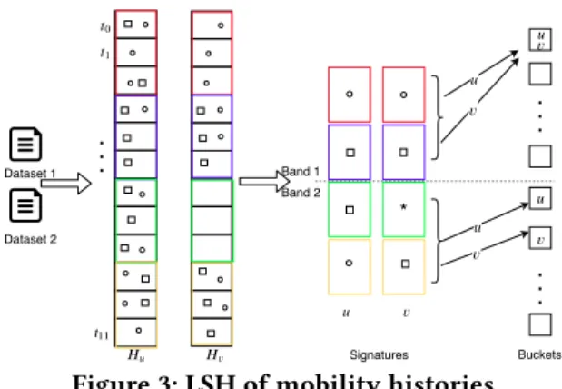
Illustrative Example. The collection of records is first con-verted into mobility histories (Figure 1). Leaf levels of the histories for two entities,u and v, are shown in Figure 3 (Hu,
Hv). In this representation, each history consists of 12 time
Buckets * Signatures Band 1 Band 2 Dataset 2 Dataset 1
Figure 3: LSH of mobility histories
windows. For illustration, we assume that entities visit only two spatial cells, represented with square and circle.
To apply LSH, we first query the mobility histories four times to identify the dominating cells. Each query has a win-dow size of three time units and is shown in different colors. The resulting signatures are of length 4. For the first query (red rectangle), the entityu visited the grid cell circle 3 times and it visited the cell square 2 times. Therefore, the domi-nating cell for entityu during the first query time window is grid-cell circle. This procedure is repeated for all queries and entities. The third index of the signature for entityv has the mark ∗ because it has no records during the third query’s time window (green rectangle). Once the signatures are ready, we apply the banding technique using two bands. For the first band, since the signatures are identical, the enti-ties are hashed to the same bucket.
Since the entitiesu and v are candidate pairs, we next compute their similarity score. In the first time window (the upper most cell),u has visited two distinct cells, circle and square, and entityv visited circle only. The pairing function N takes these two sets of locations and computes the set of record pairs to be included in the aggregation. In this exam-ple, this function pairs circles, as the distance between them are minimum (i.e., they are mutually nearest neighbors). The contribution of this pair to the similarity score is computed according to Eq 2 that takes proximity of the cells, their popularity and the length of histories into account. Last, the algorithm would check if there is an alibi pair of events in the given set. This time, we use N′as the pairing function and it
pairs square and circle grid cells as they are mutually furthest neighbors of these two sets of records. Depending on the geographical proximity of these two cells, this pair might have a negative contribution to the aggregation (alibi). This procedure will be repeated independently for each temporal window and the computed scores for each time window will be summed. Once the computation is finished, the result-ing score is used to set the weight of the edge between the entitiesu and v in the final bipartite graph.
The last step is to perform the maximum weighted bipar-tite matching and to select a subset of the resulting edges. Once the edges and their weights are determined, we fit a 1-dimensional GMM with two components over the weights of the edges and determine the stop threshold to use for linkage. We report only the edges that have higher weight than this stop threshold as a link.
5
EXPERIMENTAL EVALUATION
In this section, we give a detailed evaluation of the pro-posed solution, SLIM and compare it with state-of-the-art. We implemented SLIM using Java 1.8. All experiments were executed on a Linux server with 2 Intel Xeon E5520 2.27GHz CPUs and 64GB of RAM.
5.1
Datasets
The first set of linkage experiments is performed using the Cab dataset which contains mobility traces of approximately 530 taxis collected over 24 days (from 2008-05-17 to 2008-06-10) in San Francisco. It has 11,073,781 records. The second set of experiments is performed on linking Social Media (SM) data which contain publicly shared records with location information from Foursquare and Twitter. This dataset con-tains around 5 million records: 2,266,608 records from 197,474 Twitter users and 2,987,747 records from 276,796 Foursquare users, distributed over the globe. The dataset spans 26 days from 2017-10-03 to 2017-10-29. In the experimental evalua-tion we use only time, lat-long and anonymized user-id, and remove all other features.
In each setup (either Cab or SM), we sample two, possibly overlapping, subsets from each dataset, and link these subsets to each other. To control the experimental setup, we use two parameters during this sampling: entity intersection ratio and record inclusion probability. Intuitively, it is unlikely to have the entities from one dataset to be a subset of the other. Therefore, using the entity intersection ratio as a parameter, we control the ratio of the number entities that are common in both datasets to the number of all entities in the smaller dataset. As we show later, this parameter is critical to observe the behavior of SLIM in the presence of false positives. Once the entities are finalized, we also downsample the records from the datasets. This is to address the common case in real life that two location-based services are not always used synchronously in practice and different services might have different usage frequencies. A record of an entity is included in a dataset with the record inclusion probability. Higher probability implies denser datasets.
The default values for the entity intersection ratio, the record inclusion probability and the parameterb from Equa-tion 2 are equal to 0.5. We picked 0.5 as the default, because it is the median of all values in our experimental setup. The
spatial detail at the mobility history leaves are controlled using the cell levels of S2. A higher level indicates more spa-tial detail. The default value for the spaspa-tial level is 12, and the default temporal window width is 15 minutes. When a mobility dataset is spatially dense, using lower granularity in spatial detail results in too few spatial grid cells. Likewise, for wider temporal windows, one could expect all entities to visit all spatial grid cells. On the other hand, as we show in our experiments, using a higher spatial level of detail does not effect the accuracy but can harm the performance after a certain point. To avoid the adverse effect of entities with too small number of records after downsampling, we ignore an entity if it does not have more than 5 records. To identify the alibi threshold, we set the maximum movement speed of an entity to 2 km/minute and multiply this constant with the temporal window width. For this value, we took speed-limit of US highways into consideration.
For sections 5.2, 5.3 and 5.4 we link the datasets sampled using default parameters. For the Cab datasets we have two datasets, each with 265 entities, 133 of them are in common. Average number of events per entity in these dataset is 10,700. Similarly, for the SM dataset we have two datasets each with around 30,000 entities, and 15,000 of them are in common. Average number of events per entity in these datasets is 12.
5.2
Accuracy
In this section, we first study precision and recall as a com-posite function of the spatio-temporal level. We also look at the number of alibi entity pairs and the number of pairwise record comparisons to better understand SLIM’s behavior. Next, we studyF 1-Score and running time as a function of the record inclusion probability.
5.2.1 Effect of the Spatio-Temporal Level. Figures 4 and 5 plot precision, recall, alibi pairs and number of record com-parisons as a function of the spatio-temporal level for the Cab and SM datasets, respectively. In all figures, thex-axis shows the spatial detail, they-axis shows the width of the window in minutes, and thez-axis shows the measure.
Figures 4a and 4b show precision and recall for the Cab dataset. We observe that both measures increase with spatial detail. This is because when the spatial detail increases, the distance calculation becomes more accurate. After spatial level 12,F 1-Score becomes greater than 0.95. However, for window width, after 90 minutes, while recall remains high, precision decreases dramatically. For spatial detail 20, when the window size is 15 minutes, perfect precision is reached, while for window size 360 minutes the precision is 0.56. The decrease in precision is steeper for spatial detail 20 than spa-tial detail 16, but for the same data point recall is higher for spatial detail 20 than 16. The reason behind this is that, since the records in the same time-location bins are aggregated,
Spatial Detail 4 8 1 2 1 6 2 0 Window Width (m in) 6 0 1 2 0 1 8 0 2 4 0 3 0 0 3 6 0 Preci sion 0 .1 0 .20 .3 0 .4 0 .6 0 .7 0 .8 0 .9 1 .0 0 .6 8 0 .7 2 0 .7 6 0 .8 0 0 .8 4 0 .8 8 0 .9 2 0 .9 6 1 .0 0 (a) Precision Spatial Detail 4 8 1 2 1 6 2 0 Window Width (m in) 6 0 1 2 0 1 8 0 2 4 0 3 0 0 3 6 0 Recall 0 .10 .2 0 .3 0 .40 .6 0 .70 .8 0 .9 1 .0 0 .8 7 0 .8 8 0 .8 9 0 .9 0 0 .9 1 0 .9 2 0 .9 3 0 .9 4 0 .9 5 (b) Recall Sp atial D etail 4 8 1 2 1 6 2 0 Window Widt h (m i n) 6 0 1 2 0 1 8 0 2 4 0 3 0 0 3 6 0 A li b i (K ) 7 .8 1 5 2 3 3 1 3 8 4 6 5 4 6 2 7 0 0 5 1 0 1 5 2 0 2 5 3 0 3 5 4 0 4 5 (c) # of alibi pairs Spatial Detail 4 8 1 2 1 6 2 0 Window Width (m in) 6 0 1 2 0 1 8 0 2 4 0 3 0 0 3 6 0 R e c o rd P a ir ( B ) 7 .8 1 5 2 3 3 1 3 8 4 6 5 4 6 2 7 0 5 1 0 1 5 2 0 2 5 3 0 3 5 4 0 (d) # of event comparisons
Figure 4: Effect of the spatio-temporal level – Cab
Spatial Detail 4 8 1 2 1 6 2 0 Window Width (m in) 6 0 1 2 0 1 8 0 2 4 0 3 0 0 3 6 0 Preci sion 0 .1 0 .2 0 .3 0 .4 0 .6 0 .7 0 .8 0 .9 1 .0 0 .7 7 0 .8 0 0 .8 2 0 .8 5 0 .8 7 0 .9 0 0 .9 2 0 .9 5 0 .9 7 (a) Precision Spatial Detail 4 8 1 2 1 6 2 0 Window Width (m in) 6 0 1 2 0 1 8 0 2 4 0 3 0 0 3 6 0 Recall 0 .1 0 .2 0 .3 0 .4 0 .6 0 .7 0 .8 0 .9 1 .0 0 .5 5 0 .6 0 0 .6 5 0 .7 0 0 .7 5 0 .8 0 0 .8 5 0 .9 0 0 .9 5 (b) Recall Spatial Detail 4 8 1 2 1 6 2 0 Window Width (m in) 6 01 2 0 1 8 02 4 0 3 0 03 6 0 Alibi (M) 5 5 1 1 11 6 6 2 2 22 7 7 3 3 33 8 8 4 4 4 5 0 0 4 0 8 0 1 2 0 1 6 0 2 0 0 2 4 0 2 8 0 3 2 0 3 6 0 (c) # of alibi pairs Spatial Detail 4 8 1 2 1 6 2 0 Window Width (m in)1 2 06 0 1 8 0 2 4 0 3 0 0 3 6 0 Record Pair ( B) 0 .3 0 .6 0 .8 1 .1 1 .4 1 .7 1 .9 2 .2 2 .5 0 .2 0 .4 0 .6 0 .8 1 .0 1 .2 1 .4 (d) # of event comparisons
Figure 5: Effect of the spatio-temporal level – SM
0 20 40 60 80 100 0 10 20 30 40 50 0 100 200 300 400 0 10 20 30 40 50 60 70 80 0 1K 2K 3K 4K 0 10 20 30 40 50 60 70 80 0 5K 10K 20K 30K 35K 0 20 40 60 80 100
Figure 6: Similarity score histograms
using large time-windows makes it harder to distinguish entities from each other. When the level of detail is low, both spatially and temporally, the variance of entity pair scores is decreasing. To observe this behavior better, Figure 6 shows detected stop threshold values (red lines), fit GMM models (blue and green curves), and distribution of true positive and false positive links for spatial detail values 4, 8, 12, and 16 as a function of similarity scores for window width 90 minutes. We observe that with increasing spatial detail, grouping true positive links (green bars) and false positive links (blue bars) in two clusters becomes more accurate and a tighter stop threshold value could be identified. By looking at the dis-tances between two components of GMM one could say that stop threshold identification has subpar accuracy for spatial detail values lower than 12. One could observe this subpar accuracy by looking at the differences between precision
behaviors of Figures 4a and 5a. We observe similar results using Otsu technique [27] and 2-means clustering but those experiments are omitted due to space constraints. For low spatial detail (i.e., ≤ 10) and high temporal window width (i.e., ≥ 60 minutes), precision is favored over recall for the Cab dataset but vice-versa for SM.
While spatial level values higher than 12 have similar precision and recall, we observe that increasing spatial detail also increases the number of record comparisons. This is expected, as we discussed in Section 3.3 how to use the trade-off between accuracy and performance to detect the best spatial detail for a given temporal window. When the window size is 15 minutes, the spatial detail detected by the parameter tuning algorithm is 12. Figure 4d shows that for the same window width, increasing spatial detail from 12 to 20 increases the number of pairwise record comparisons by 1.14 times, yet the accuracy stays the same. The gap widens for longer temporal windows. The same figure shows 3.15× increase in the number of record comparisons when the window size is increased from 15 to 360 minutes, for spatial detail 12. Yet, the increase is 22× for spatial detail 20.
Figure 5 shows the same experiment for the SM dataset. Most of the previous observations hold for this dataset as well. There are two additional observations. First, in the Cab dataset the best recall value is reached when 5-minute win-dows are used. This is a result of the spatio-temporal density of the Cab dataset, as alibi detection becomes more efficient for narrow windows, resulting in better recall. On the other
0 .1 0 .3 0 .5 0 .7 Inclusion Probability 0 .0 0 .2 0 .4 0 .6 0 .8 1 .0 F1 Scor e 0.5 0.7 0.9 0.3 0.9
(a) F1-Score – Cab
0 .1 0 .3 0 .5 0 .7 Inclusion Probability 6 0 0 8 0 0 1 0 0 0 1 2 0 0 1 4 0 0 1 6 0 0 1 8 0 0 2 0 0 0 2 2 0 0 Runtime (sec) 0.5 0.7 0.9 0.3 0.9 (b) Runtime – Cab 0 .1 0 .3 0 .5 0 .7 Inclusion Probability 0 .0 0 .2 0 .4 0 .6 0 .8 1 .0 F1 S cor e 0.5 0.7 0.9 0.3 0.9 (c) F1-Score – SM 0 .1 0 .3 0 .5 0 .7 Inclusion Probability 0 5 0 0 1 0 0 0 1 5 0 0 2 0 0 0 2 5 0 0 3 0 0 0 3 5 0 0 Runtime (sec) 0.5 0.7 0.9 0.3 0.9 (d) Runtime – SM
Figure 7: F1-Score and Runtime as a function of the inclusion probability (for different entity intersection ratios)
Spatial Detail 4 8 1 2 1 6 2 0 Temporal Steps 0 5 0 1 0 0 1 5 0 2 0 0 Relative F1 Score 0 .0 0 .1 0 .2 0 .3 0 .4 0 .6 0 .7 0 .8 0 .9 1 .0 0 .8 0 0 .8 2 0 .8 4 0 .8 6 0 .8 8 0 .9 0 0 .9 2 0 .9 4 0 .9 6
(a)F 1-Score – Cab
Spatial Detail 4 8 1 2 1 6 2 0 Temporal Steps 0 5 0 1 0 0 1 5 0 2 0 0 Speed Up 0 .0 3 8 7 7 1 1 6 1 5 5 1 9 4 2 3 3 2 7 2 3 1 1 3 5 0 2 5 5 0 7 5 1 0 0 1 2 5 1 5 0 1 7 5 2 0 0 (b) Speed-up – Cab Spatial Detail 4 8 1 2 1 6 2 0 Temporal Steps 0 5 0 1 0 0 1 5 0 2 0 0 Relative F1 Score 0 .0 0 .1 0 .2 0 .3 0 .4 0 .6 0 .7 0 .8 0 .9 1 .0 0 .7 8 0 .8 0 0 .8 2 0 .8 4 0 .8 6 0 .8 8 0 .9 0 0 .9 2 0 .9 4 (c)F 1-Score – SM Spatial Detail 4 8 1 2 1 6 2 0 Tem poral Steps 0 5 0 1 0 0 1 5 0 2 0 0 Speed Up 0 .0 1 5 5 3 1 1 4 6 6 6 2 2 7 7 7 9 3 3 1 0 8 8 1 2 4 4 1 4 0 0 1 5 0 3 0 0 4 5 0 6 0 0 7 5 0 9 0 0 1 0 5 0 1 2 0 0 (d) Speed-up – SM
Figure 8: LSH accuracy and speed-up as a function of the spatial level and temporal step size
28 210 212 214 216 218 220 Number of Buckets 0 2 0 0 4 0 0 6 0 0 8 0 0 1 0 0 0 1 2 0 0 Speed Up 0.4 0.5 0.6 0.7 0.8
(a) Speed-up – Cab
28 210 212 214 216 218 220 Number of Buckets 0 5 1 0 1 5 2 0 2 5 3 0 Speed Up (K) 0.4 0.5 0.6 0.7 0.8 (b) Speed-up – SM
Figure 9: Speed-up as a function of the bucket size hand, in the SM dataset, the best recall is reached for 15-minute windows. This is expected, because at one extreme very small temporal windows require services to be used synchronously to collect evidence for linkage. Another obser-vation is that, as SM dataset has lower spatio-temporal skew, to detect alibis one needs to use larger temporal windows. 5.2.2 Sensitivity to the Workload Parameters. In this experi-ment, we link one dataset of each source with the datasets sampled with different entity intersection ratios and record inclusion probabilities. Figure 7 plots theF 1-Score and run-ning time in seconds as a function of record inclusion prob-ability for the Cab and SM datasets, respectively. Different series represent different entity intersection ratios. The Cab dataset has 265 entities and the SM dataset has around 30,000 entities. The average number of records for an entity is rang-ing from 2,100 to 18,900 for the Cab dataset and from 10 to 20 for the SM dataset. Figure 7a shows the results for the Cab dataset. We observe that allF 1-Score values are close to 1, even when average number of records are as low as
2,100 (inclusion probability 0.1). Moreover, from Figure 7b, we observe that the running time is sub-linear with average number of records, which is a result of aggregation on mo-bility histories. These results validate robustness of SLIM, as F 1-Score is not effected by the increasing number of records and the system scales linearly.
8 10 12 14 16 18 20 22 24 Sp at ial Lev el 0.0 0.2 0.4 0.6 0.8 1.0 F 1 S c o re Original MNN All_Pairs No IDF No Normalization
(a) F1-Score Spatial Level
0 100 200 300 400 500 600 700 800 W in d ow W id t h 0.0 0.2 0.4 0.6 0.8 1.0 F 1 S c o re Original MNN All_Pairs No IDF No Normalization
(b) F1-Score Window Width
Figure 10: Ablation Study
Figures 7c and 7d show the results of the same experi-ment for the SM dataset. Different than the Cab dataset, the effect of the record inclusion probability on theF 1-Score is more pronounced here. For the entity intersection ratio value of 0.5, the average number of records is 10,F 1-Score is 0.75. When the average number of records is doubled, we get 0.98 as theF 1-Score. This is because the average number of records per entity is already low in the SM dataset and down-sampling it to even lower values decreases the number of records that can serve as evidence for linkage. However, we observe that SLIM is able to perform high-accuracy linkage when the average number of records per entity is at least 15. Independent of the entity intersection ratio, after 15 records
per entity, theF 1-Score of SLIM is greater than 0.9. Similar to Cab dataset, the running time of SLIM is linear with the input size for SM dataset.
5.3
Scalability
In this set of experiments, we study the effect of the LSH on the quality and the scalability of the linkage. The qual-ity is measured using theF 1-Score relative to that of the brute force linkage. LetF Score where LSH is applied be F 1-Scorelshand without itF 1-Scorebf. Then, relativeF 1-Score
equalsF 1-Scorelsh/F 1-Scorebf. Likewise, to measure the
speed-up, we compute the ratio of the number of pairwise record comparisons without LSH to that of with LSH. 5.3.1 Effect of the Spatio-Temporal Level. Figure 8 shows the relativeF 1-Score and the speed-up as a composite function of the spatial level and the temporal step size. Recall that we construct a set of dominating cells to act as signatures. This construction is done by querying each mobility history for non-overlapping time windows. The size of each grid cell is defined by the spatial level. The temporal step size represents the number of time windows the query spans. Note that these parameters are different than the spatial level and the window width that is used for the similarity score computation. The LSH similarity thresholdt is set to 0.6 and the number of buckets is set to 4096.
Figures 8a and 8b show the relativeF 1-Score and speed-up, respectively, for the Cab dataset. Figure 8a shows that theF 1-Score achieved with and without LSH are almost the same when the spatial level is lower than 12. Similarly, we do not observe any speed-up for these data points. The reason is that the Cab dataset is spatially too dense and consequently dominating grid cells of all entities end up being the same when the spatial detail is low. However, when the spatial detail is increased, we observe that LSH brings 2 orders of magnitude speed-up by preserving 98% of theF 1-Score. For the spatial detail value of 16 and temporal step size of 48 (this means each dominating grid cell query spans 12 hours) the speed up reaches 202×. The maximum speed-up achieved for this dataset is 332×, preserving 86% of theF 1-Score.
Figures 8c and 8d present the same experiment for the SM dataset. While we observe similar behavior for low spatial detail, we also observe that the increase in the speed-up starts earlier and is steeper when the spatial detail is increased. This is because the SM dataset has lower geographic and temporal skew. If we observe the same data point as we did with the Cab dataset, we observe more pronounced speed-ups: For the spatial detail value of 16 and temporal step size of 48, LSH brings 1177× speed-up preserving 91% of theF 1-Score. Next, we show that the maximum reachable speed-up is much higher when the number of buckets is increased.
5.3.2 Effect of the LSH Parameters. Figure 9 plots the speed-up as a function of the number of hash buckets. Different series represent different LSH similarity thresholds. We set the spatial detail and temporal step size of the signature calculation to 16 and 48, respectively.
Intuitively,F 1-Score is not effected by the number of buck-ets. This is because if two entities have at least one identical band in their signatures, they are hashed to the same bucket independent from the number of buckets. Yet, increased num-ber of buckets increases the speed up as the probability of hash collision decreases. Similarly, the LSH similarity thresh-old affects the relativeF 1-Score. This is because, its smaller values increase the probability of becoming a candidate pair. We observe the increase in speed-up for the Cab dataset and the SM dataset in Figures 9a and 9b, respectively. When the number of buckets is set to 218and the similarity thresh-old is set to 0.6, the speed-up becomes 380× with a relative F 1-Score of 0.98 for the Cab dataset and 11,742× with a rela-tiveF 1-Score of 0.91 for the SM dataset. Since the number of entities in the SM dataset is much larger compared to the Cab dataset, we observe a significant difference in speed-up.
5.4
Ablation Study
In this experiment, we observe how the building blocks of SLIM work together and provide robustness against chang-ing spatio-temporal level of detail. This includes the effect of using mutually nearest and furthest neighbors, normaliza-tion, and IDF components via varying the spatial detail and window width. Figures 10a and 10b show theF 1-Score as a function of the spatial detail and window width, respectively. Each line represents a different modification to SLIM.
SLIM matches mutually nearest neighbor event pairs in the similarity computation. It also has an optional step in which the mutually furthest pairs are computed to further support the alibi detection. To compare this approach with other blocking techniques we use two lines. First, the purple line with circle markers (MNN) represents the case where this optional step is removed. Second, the blue line with star markers (All Pairs) represents the case where we match all pairs of events. From Figure 10a, we observe all three blocking techniques used have similarF 1-Score values. This is because, the temporal window is narrow (15 minutes), and the number of events in each window is already low. At one extreme, if two mobility records have only one event at the same temporal bin, all techniques will return the same pair. Supporting this observation, in Figure 10b we observe theF 1-Score of All Pairs decrease dramatically when wider temporal windows are used. For temporal level of 720 minutes, while the original algorithm and MNN have 0.90F 1-Score, that of All Pairs is only 0.61. While the effect of the optional MFN step is not obvious for this setting, when we look at the
(a) Hit precision @40 102 103 104 105 R u n ti m e ( S e c ) 20 40 80 165 330 660 Avg Num ber of Records (vs 675) 0.0 0.2 0.4 0.6 0.8 F 1 S c o re (b)F 1-Score (c)F 1-Score 102 103 Runtime (Sec) 2100 6300 10500 14700 18900 Avg Number of Records (vs 10750) 108 1010 Record Compar isons (d) Record comparisons
Figure 11: Comparison with existing work (Sub-figures a and b, and c and d are sharing their legends) linked pairs, we observe that this step decreases the similarity
score of false positive pairs. For spatial level 12 and temporal level 5 minutes, the mean of the similarity score of the false positive pairs decreases from 2227 to 1501. This indicates that capturing the alibi pairs is harder with MNN only, and the effects of the optional MFN step is significant.
Next, we observe the effects of the normalization and IDF components of the similarity score computation. Red line with cross markers (No IDF) represents the case where IDF is removed, and green line with triangle markers (No Normal-ization) represents the case where normalization is removed. Figure 10a shows that the effect of normalization gets more significant with increasing spatial level of detail. For spatial level 24 and temporal level 15 minutes, we observeF 1-Score of the original algorithm is 0.96, while that of No Normaliza-tion is 0.76. When the temporal window is wider, one can observe the significance of the IDF component. For window width 720 minutes,F 1-Score of SLIM is 0.89, while that of No IDF is 0.69. This is because, awarding uniqueness becomes even more important, since the unique time-location bins are rarer in wider temporal windows.
5.5
Comparison with Existing Work
We compare SLIM with the two existing approaches. First is GM3, which works by learning mobility models from entity records using Gaussian Mixtures and Markov-based mod-els [43]. These modmod-els are later used for estimating the miss-ing locations of users, and also settmiss-ing weights to spatio-temporally close record pairs. While we only check records those are in the same temporal window, they also award pair of records those are from different temporal windows.
Second is ST-Link, which performs a sliding-window based comparison over the records of entities and links them if they havek co-occurring records in l diverse locations, and no alibi record pairs [3]. If an entity has such co-occurring record pairs with more than one entities from the other dataset, all pairs are considered ambiguous and ignored. To identify the values ofk and l, a trade-off point is identified based on the distribution of allk and l-values [3].
3We used the code from the authors: https://tinyurl.com/yagfaz5n
We do not compare our approach with other existing ap-proaches because in its paper GM outperforms eight other approaches, excluding ST-Link. ForF 1-Score comparisons we also include no-LSH SLIM algorithm. For other data points, we apply LSH with 4096 buckets andt equals 0.6.
Hit Precision @k is calculated independently for all enti-ties via the formula 1 −max((rank/k), 1) and averaged. The rank is the order of the true link in the list of all entities from the opposite dataset, sorted in decreasing order of their similarity score. Figures 11a and 11b show the Hit Precision @40, running times, andF 1-Score as a function of the aver-age number of records. Figure 11b also shows the no-LSH SLIM algorithm, represented with single hatched bar and solid line. Since GM does not implement any mechanism to scale to a large number of records, to include it in our re-sults, we took a 1 week subset of the data. The pivot dataset has 265 taxis with 675 records on average. We sampled 5 other datasets, with changing number of average number of records, ranging from 20 to 660. These datasets have 265 taxis, 133 of which are common with the pivot. With this setting the best achievable hit precision is 0.5.
From these two figures, we observe that the hit precision values for GM is increasing as the average number of records increases. ST-Link reaches the maximum hit precision with as small as 20 records. SLIM outperforms GM in all data points, and reaches its best hit precision when the average number of records is 165. While all three algorithms are able to provide perfect hit precision @40, their performance in terms ofF 1-Score differs dramatically. When the average number of records is 20, SLIM reaches anF 1-Score of 0.3, while the other two alternatives stay around 0.05. Since GM does not link entities with a single entity from the opposite dataset, we apply our linkage and stop threshold algorithm over their similarity scores. While ST-Link is able to rank true positive pairs at the top (we could conclude this from perfect hit precision), it is not always able to detect correctk and l values and resolve ambiguity. When the number of average records per entity increases to 660, we observe that SLIM still performs the best in terms of theF 1-Score with 0.92, while SLIM with LSH shows a similar performance of accuracy
with 0.89F 1− Score. For the same data point, ST-Link and GM haveF 1-Scores of 0.87 and 0.73, respectively.
From the running time experiments we observe that GM is two orders of magnitude slower than the other two algorithms. Therefore, we exclude GM in further experi-ments. Likewise, we exclude no-LSH SLIM algorithm. Fig-ures 11c and 11d showF 1-Score, the running times and num-ber of pairwise record comparisons for different record den-sities, respectively. Green bars correspond to SLIM, the red bars to ST-Link. We use two different intersection amount ratios for each data point. Bars with single hatches show the results for intersection ratio 0.3, and double hatches show that of 0.7. We observe that SLIM outperforms ST-Link in terms ofF 1-Score in all data points except one, and accuracy of ST-Link decreases when the average number of records per entity increases. This is because SLIM is more robust to alibi record pairs than ST-Link, even when alibi threshold mechanism of ST-Link is used. In this experiment, we set the alibi threshold count to 3 for ST-Link.
Figure 11d shows that SLIM makes three orders of magni-tude less pairwise record comparisons than ST-Link. Like-wise, we observe SLIM runs much faster than ST-Link. For average number of records 18,900, with intersection ration 0.3, the running time of the SLIM is 343 seconds, while that of ST-Link takes 1096 seconds. This is mainly due to the ef-fectiveness of the proposed LSH-based scalability technique.
6
RELATED WORK
Many of the attempts in user identity linkage (aka user rec-onciliation as surveyed in [38]) utilize additional information such as the network [20, 23, 42], profile information (such as usernames or photos) [14, 26, 37], semantic information related to locations [24], or a combination of these [25, 46]. However, in many cases, only the spatio-temporal informa-tion is present or can be used in mobility data, and many of the other identifiers are likely to be anonymized. Use of only spatio-temporal information also aligns better with the new regulations of minimal data collection with consent.
Defining a location based similarity between entities is a fundamental problem [17, 45]. Some express this based on densities of location histories [13], either by matching user histograms [41], or using the frequencies of visits to specific locations during specific times [35]. Statistical learning ap-proaches are also used to relate social media datasets with Call Detail Records [5, 6]. However, these algorithms depend on discriminative patterns of entities, which is not likely to be present in many datasets, such as the taxi datasets.
There have been recent studies to define the similarity among entities using the co-occurrences of their records [3, 4, 19, 32, 43]. These are the most related group of work to ours, and two of them (ST-Link [3], GM [43]) are included in
our experimental evaluation. SLIM is shown to outperform them in terms of both accuracy and scalability. Some of these algorithms (GM and Pois [32]) depend on an assumed model for the users. For example, Pois assumes that visits of each user to a location during a time period follows Poisson distribution and records on each service are independent from each other following Bernoulli distribution. In contrast, we do not make any mobility model assumptions and can work solely on raw spatio-temporal information. Moreover, these work do not address scalability. We introduce an LSH based solution to scale the linkage process.
Cao et al. [4] define the strength of the co-occurrences inversely proportional with the frequency of locations. A multi-resolution filtering step is developed for scalability. Different from our approach, the data is pre-processed to add semantic information to locations. They do not define a concept of dissimilarity, which is shown to improve both accuracy and efficiency in our solution. Also, they do not au-tomatically determine a similarity threshold to stop linkage. Trajectory similarity is usually measured using subse-quence similarity measures such as the length of the longest common subsequence, Frechet distance, or dynamic time warping[1]. There are trajectory specific techniques that in-clude information like speed, acceleration, and direction of movement [18]. In contrast to our work, these approaches have strong assumptions, they fell short in addressing asyn-chrony of the datasets and capturing alibi event pairs. Our approach is more generic as it depends on less features when computing similarity and linkage.
7
CONCLUSION
In this paper, we studied the problem of identifying the matching entities across mobility datasets using only spatio-temporal information. For this, we first developed a summary representation of mobility records of the entities and a novel way to compute a similarity score among these summaries. This score captures the closeness in time and location of the records, while not penalizing temporal asynchrony. We ap-plied a bipartite matching process to identify the final linked entity pairs, using a stop similarity threshold for the linkage. This threshold is determined by fitting a mixture model over similarity scores to minimize the expectedF 1-Score metric. We also addressed the scalability challenge and employed an LSH based approach for mobility histories, which avoids unnecessary pairwise comparisons. To realize effectiveness of the techniques in practice, we implemented an algorithm called SLIM. Our experiments showed that SLIM outperforms two existing approaches in terms of accuracy and scalabil-ity. Moreover, LSH brings two to four orders of magnitude speed-up to the linkage in our experimental settings.