IEEE TRANSACTIONS ON INFORMATION THEORY, VOL. 38, NO. 6, NOVEMBER 1992
~
1833
TABLE XI
WEIGHT ENUMERATOR OF
ck ,
A [52,27,9]-CODE 1+
170~’+ 442~’”
+ 714y”
+
6188~”+ 28560~”
+5304Oyl4+ 77520~”
+ 3 0 8 9 5 8 ~ ’ ~
+ 8 7 9 4 8 0 ~ ’ ~
+
1270360y’8 + 1661240y” + 3754569~”+ 6824752~‘~
+ 8 0 6 5 6 1 6 ~ ~ ~+ 9306480~’~
+
1270750Oyz4+ 14775.516~~~
+
14775516~‘~+ 14775516~”
+ 12707500yZ8
+ 9306480~’~
+8O65616y3O + 6 8 2 4 7 5 2 ~ ~ ~+
37.54569~~~+
1 6 6 1 2 4 0 ~ ~ ~+
1270360~1~~+
879480~”+ 3 0 8 9 5 8 ~ ~ ~
+
7 7 5 2 0 ~ ~ ~ +53040y3+ 2 8 5 6 0 ~ ~ ~
+ 6 1 8 8 ~ ~ ’
+ 714y41
+ 4 4 2 ~ ~ ~
+ 1 7 0 ~ ~ ~+
y5’ TABLE XI1A GENERATOR MATRIX AND WEIGHT DISTRIBUTION OF T54, A [54,27,10]-CODE 1000000000000000000000000000001 110101 11 1000001 11 100010 01000000000000000oO00000100000100111011101000011100100 001000o0O000000m0000100011100101001001011001001111 00010000000000000000000010000l010100l11111011101011111 000010000000OOOO0010101001001101oO0110011000 000001000000000000000000l00010100000001010100001010010 0000001000000000000000001000000l1011101111110100100100 00000001000000000000oO00000010110010110001011100000001 000000001oO0000000000000000011110000010101101000011000 0000000001000000000000001000001 1 1 1010100001 1001 0000010 00000000001000000000000000001010000110l110111111010010 0000000000010000000000000000101 11001 1 1101001 1001 110001 000000000000100oO0000000000011110101110000001010100000 000000000000010000000000100000111111 1000100000110111 10 00000000000000100000000000001010000011011 110011 1111100 000000000000000100000OOOlOOOOOO10101ooo0011101011 loo00 0000000000000000100000001000000110011 1000101110011 1101 00000000000000000 1000000 10000 10 1 1 1 1 1 10 100 100 100001 101 1 000000000000000000100000100001 11 1100100101000010001000 00oO00000000000000010000000010000001010100000111010111 00000000000000000000100000001 1101001 1001 1 100010 I 1 1001 1 000000000000000000000 1000000 1 10 1 1 10 1 1 1 1 1 10 100 100 100001 0000000000000000000000100000l1000111110010010100001000 00000000000000oO00000001000010001010110100001100011100 0000000000000000000000000100101 1 1 11 10001 101001 1001001 1 00000000000000000000000oO010 1 1 1 10 1 10 10 1 1 1001 0 10 10 1000 1 000000000000000000000oO000011101001001101000110011oO00 Weight Frequency 0 1 10 255 12 5831 14 44268 16 330174 18 1414284 20 4802364 22 11681 193 24 20802220 26 28028274 28 28028274 30 20802220 32 1 168 1193 34 4802364 36 14 14284 38 330174 40 44268 42 5831 44 255 54 1 ~~
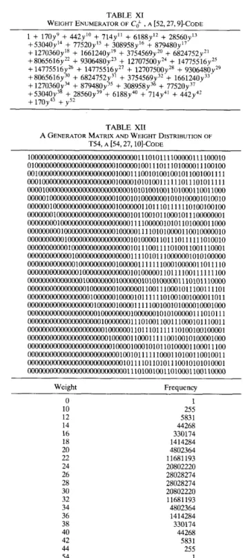
MacWilliams identities, the weight enumerator of Ck is shown in Table XI. Let S be a codeword in C that is not orthogonal to s, where
S = (100000000000000000000000001 11 11
00010 10000 1 1 10100 100 1).
TABLE XI11
WEIGHT ENUMERATOR OF
(c,*)’
, A [54,28,3]-CODE 1+
y 3+
255y”+
2754 “+
5 8 3 1 ~ ’ ~+
4 4 2 6 8 ~ ’ ~ +258944yI5+
330174~‘+
1414284~’~+
5469039~”+
4802364~’~+
11681193y”+
3 2 3 7 2 3 5 2 ~ ~ ~+ 2 0 8 0 2 2 2 0 ~ ~ ~
+
2 8 0 2 8 2 7 4 ~ ~ ~+ 58011548~’~
+
28028274~’~+
2080222Oy3O +32372352y3‘+
11681193y3’+
4 8 0 2 3 6 4 ~ ~ ~+ 5469039~~
+
1 4 1 4 2 8 4 ~ ~ ~+
3 3 0 1 7 4 ~ ~ ~+
258944~~’+
4 4 2 6 8 ~ ~ ’ +5831y4’+
2 7 5 4 ~ ~ ~+
2 5 5 ~ ~ ~+
y51+
y S 4By Theorem 1, we get a new code C*, which we denote by T54, a [54,27,10]-code, which is generated by (1,0, s), (1,1, S ) and 25
basis vectors of CO, (0, 0, basis vector of CO>. A generator matrix and the weight distribution of T54 are shown in Table XII. Hence, we get W as given in (4) with
p
= 12.Let C,* be the subcode of C* consisting of all codewords of weight O(mod 4). Then (e,*) has the weight enumerator, by the MacWilliams identities, as shown in Table XIII. Therefore, we get S in (4) with
p
= 12.ACKNOWLEDGMENT
The author would like to thank Prof. J. Leon for his fast program help and for comments on the manuscript. The author would also like to thank Prof. V. Pless for her lecture discus- sions.
REFERENCES
[1] J. H. Conway and N. J. A. Sloane, “A new upper bound on the minimal distance of self-dual codes,” IEEE Trans. Inform. Theory,
vol. 36, pp. 1319-1333, NOV. 1990.
R. A. Brualdi and V. S. Pless, “Weight enumerators of self-dual codes,” IEEE Trans. Inform. Theory, vol. 37, pp. 1222-1225, July 1991.
[3] H. P. Tsai, “Existence of certain extrema1 self-dual codes,” IEEE Trans. Inform. Theory, vol. 38, pp. 501-504, Mar. 1992.
[2]
Sequential Decoding of Low-Density Parity-Check Codes by Adaptive
Reordering of Parity Checks
Branko Radosavljevic, Student Member, IEEE, Erdal Arikan,
Member, IEEE, and Bruce Hajek, Fellow, IEEE
Abstract-Decoding algorithms are investigated in which unpruned codeword trees are generated from an ordered list of parity checks. The order is computed from the received message, and low-density parity- check codes are used to help control the growth of the tree. Simulation results are given for the binary erasure channel. They suggest that for
Manuscript received November 15, 1990; revised November 15, 1991.
This work was supported by the Joint Services Electronics Program under Grant N00014-90-5-1270 and by an Office of Naval Research graduate fellowship. This work was presented in part at the IEEE International Symposium on Information Theory, Budapest, Hungary, June 24-28, 1991.
B. Radosavljevic and B. Hajek are with the Coordinated Science Laboratory and the Department of Electrical and Computer Engineer- ing, University of Illinois, Urbana, IL 61801.
E. Arikan is with the Department of Electrical Engineering, Bilkent University, P.K. 8, 06572, Maltepe, Ankara, Turkey.
IEEE Log Number 9203035. 0018-9448/92$03.00 0 1992 IEEE
small erasure probability, the method is computationally feasible at rates above the computational cutoff rate.
Index Term-Low-density codes, sequential decoding, computational cutoff rate.
I. INTRODUCTION
Sequential decoding is a general method for decoding tree codes. The amount of computation depends on the channel noise and the expected computation per decoded digit is finite only at code rates below R,, the computational cutoff rate. The present scheme is a modification of standard sequential decod- ing in an attempt to operate at rates greater than R,.
With standard sequential decoding, a long burst of noise requires a great deal of computation to resolve. This is illus- trated in the following example, taken from [7]. Suppose we have a binary erasure channel and use a convolutional code with rate R. If the first L symbols are erased, then each path with length
L symbols in the codeword tree will appear equally likely to the
decoder, until they are extended further into the tree. Since there are approximately 2 L R such paths, and each path has
probability 1/2 of being extended before the decoder finds the correct one, the expected number of paths searched by the decoder is 2LR-’. A long burst of noise will cause a sequential decoder to perform a great deal of computation even on more general communication channels. For example, consideration of bursts allowed Jacobs and Berlekamp [7] to prove their proba- bilistic lower bound to the amount of computation on any discrete memoryless channel.
This leads one to consider adaptively reordering the codeword tree, that is, changing the order of the digits used to generate the tree. In this way, one can try to limit the occurrence and duration of bursts of noise. More generally, the goal of reorder- ing the tree is to decrease the computation performed by the sequential decoder.
Apparently, however, one cannot significantly reorder the codeword tree associated with a convolutional code and still obtain a tree that is practical to search. Instead, in this paper we consider decoding linear block codes by sequential decoding. Our method of generating codeword trees for block codes differs from that taken by Wolf [lo], Forney [3], and others. The nodes of the trees that we construct are partially specified n-tuples which may correspond to valid codewords. If the trees were suitably pruned, the nodes would always correspond to partially specified codewords, and thus, we call our trees unpruned code-
word trees.’ In contrast, the nodes in Wolfs trellis correspond to parity check sums of partially specified n-tuples. A similar prun- ing operation in his case leaves only those paths in the trellis that correspond to partially specified codewords. In addition, the resulting trellis is typically decoded using Viterbi decoding in- stead of sequential decoding.
Specifically, we consider using low-density parity-check codes. These codes, devised by Gallager [5], [6], are linear block codes characterized by three parameters. A b i n a j ( n , q, r ) low-density code has blocklength n, and a parity matrix with exactly q 1’s in each column and r 1’s in each row. Typically, q and r are much smaller than n , resulting in a sparse parity matrix. For these reasons, low-density codes have the following two features. First, given any ordering of the parity checks used to define a low-den- sity code, one can generate an unpruned codeword tree that
’
Although we do not explicitly prune the tree, the decoding algorithm essentially does this automatically, by choosing trees in which invalid turns quickly lead to dead ends.Ordering Algorithm
Decoder
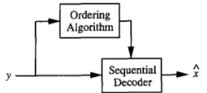
Y
Fig. 1. The general structure of SDR algorithms.
grows slowly compared to the growth for a dense parity matrix. Second, different parity check orderings yield different trees.
These two features are used by the decoding algorithms presented in this correspondence. The algorithms, which we call sequential decoding with reordering (SDR) algorithms, all have the structure shown in Fig. 1. The ordering algorithm observes the channel output and uses this information to choose a parity check ordering. The sequential decoder then searches the corre- sponding tree to obtain the decoder output. Decoding algo- rithms are discussed for the binary erasure and binary symmetric channels. Simulations were performed to investigate the possibil- ity of using this approach at rates greater than R,.
There exist other methods related to sequential decoding that can operate at rates greater than R,. In one approach, due to Falconer [2], codewords of a block code with blocklength N are fed in parallel to N convolutional encoders. The result is de-
coded by N parallel sequential decoders, and the structure of
the block code is used to push forward the slowest sequential decoders. A second approach, considered by Pinsker [8], uses concatenated codes, where the inner code is a block code and the outer code is a convolutional code. Both approaches can operate at rates up to capacity. In related research, other decoding algorithms for low-density codes have been presented by Gallager [SI, [6, pp. 41-52, 57-59] and Zyablov and Pinsker We use the following terminology. The vector x = ( x ~ ) : , ~ is the transmitted codeword and y = (y,):, is the channel output, where n is the blocklength of the code being used. For simplic- ity, we assume the channel input is binary.
[111, 1121.
11. CODEWORD TREES FOR L ~ W - D E N S I T ~ CODES To begin with, we mention some relevant properties of a binary ( n , q , r ) low-density code. There are nq/r rows in the parity matrix, but the rows need not be linearly independent. Thus, the rate R satisfies
R 2 1 - q / r .
We use this bound to approximate R . One expects this approxi-
mation to be good for the codes used in this study because the parity checks are randomly chosen (using a construction similar to that given in [ 5 ] , [6, pp. 12-13]). A second property, obtained by Gallager [SI, [6, p. 161, is that with q and r fixed with q 2 3,
the typical minimum distance of a random low-density code grows linearly with n. Finally, codes in this study are chosen to satisfy two constraints: n is a multiple of r , and no two parity check sets have more than one digit in common. The first constraint is required by the code construction procedure. The second constraint was desirable when using the decoding algo- rithms considered for the binary symmetric channel, and in addition prevented the degenerate case of having a code with minimum distance equal to two.
To generate an unpruned codeword tree, we start with an ordered list of the nq/r parity equations used to define the
IEEE TRANSACTIONS ON INFORMATION THEORY, VOL. 38, NO. 6, NOVEMBER 1992 1835 6j Parity equations X I + x* + X j x3 + x q + x5 x s + x a + x , = o 0 0 0 1 ... - Example:
Binary erasure channel
y = OeeelOl Level 0 1 2 3 4
E
l
OIlOIlO 01110 - - 10101 . . 1011ooo 101 .... 10110.- “--:ew
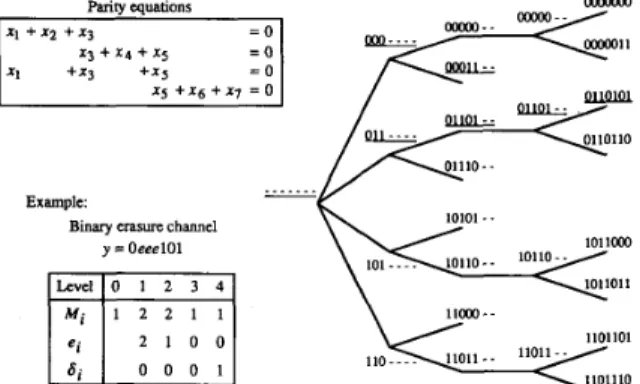
1011011Fig. 2. An unpruned codeword tree for a linear block code defined by
four parity equations. (To conserve space, the code is not a low-density code.) Nodes that agree with the received message have underlined labels. The quantities Mi, ei, and 6, are defined in Section IV.
code. (See Fig. 2.) Any ordering will work; at this point it is arbitrary. Each parity check corresponds to a level in the tree, and the nodes of the tree correspond to partially specified n-tuples.
At the root node, the n-tuple is completely unspecified. In moving from a node to one of its children, the set of specified digits is increased by those “new” digits (if any) that appear in the current parity check but not in any previous parity check. A different child is created for each of the ways to assign values to these new digits that satisfies the current parity check. Note the possibility that all the digits involved in the current parity check have already been assigned values earlier in the tree (i.e., the current parity check contains no new digits). In this case, a node will have no children if it does not satisfy the current parity check. For this reason, the tree is called “unpruned,” to stress the fact that some nodes at intermediate levels may not corre- spond to valid codewords.
Thus, a given level in the tree consists of all the subsequences that satisfy the current and all previous parity checks. At the final level, all the n-tuples are completely specified, and they all correspond to valid codewords.
This procedure can be used with any linear block code. However, in the general case there is no limit on the number of digits involved in a parity check, other than the blocklength n. A typical parity check may involve n / 2 digits. If this is the first parity check used to generate the tree, there will be 2n/2-1 nodes in the first level, and this is too large to be searched by a practical decoder. However, in an ( n , q, r ) low-density code,
each parity check used to define the code involves exactly r
digits. The parameter r is typically small, and may be chosen
independently of n. All low-density codes considered here have
r I 10. As discussed next, trees for low-density codes have fanout limited by 2 * - ’ , and typically the fanout is much less.
One property of the trees obtained using the method previ- ously given is the variability of their fanout, or growth rate. This contrasts with codeword trees for convolutional codes, which grow at the same rate at every level. To characterize the growth rate, we first present some definitions. The set of digits involved in a parity check is referred to as a parity check set. Given an ordering of the parity checks, each parity check set is partitioned into two groups, the n-set and the o-set. The n-set, or new set, contains the “new” digits (as previously defined), and the o-set, or old set, contains the rest.
Given a tree for an ( n , q , r ) low-density code, let ni be the
number of digits in the n-set associated with level i in the tree. Also, let
4.
be the total number of nodes at level i, with No= 1. Then it is not hard to check that, for 1
I i1) if the ith parity check is independent of the preceding
n q / r ,
parity checks,
2) otherwise,
Ni
= N i - l .In general,
This result implies that codeword trees for low-density codes tend to grow quickly near the beginning of the tree and more slowly toward the end. This occurs because the growth rate at a given level depends on the size of the corresponding n-set. At a level close to the origin, few digits will have had a chance to appear in previous parity check sets, hence the corresponding n-set tends to be large. The opposite situation holds near the end of the tree. As a result, ni will roughly be a decreasing function of i. This is not a hard and fast rule, but a good qualitative description that holds regardless of which parity check ordering is used.
In addition to the variable growth rate, codeword trees for low-density codes and those for convolutional codes differ in another important way. With a low-density code, two different subtrees descending from a common parent node can be identi- cal for many levels. This happens because the set of digit values assigned to a node’s children depends only on the parity of the child level’s o-set. Specifically, two subtrees with a common parent node will agree on the values they assign to codeword digits until a level is reached where the o-set in one subtree has different parity than the o-set in the other subtree. To deter- mine where such a level can occur, consider the root nodes of the two subtrees. The labels of these two nodes will differ only in the values assigned to the digits in the n-set of the level containing the root nodes. Denote this n-set by S. Then the first level at which the two subtrees can differ must have an o-set that contains one or more digits in S.
This property can significantly affect the behavior of a sequen- tial decoder. If the decoder diverges from the correct path in the tree, it may not be able to detect its error for many levels. In this case, backtracking one level at a time would be very inefficient. For example, when using a (396,5,6) low-density code and a typical parity check ordering, ten percent of the digits will have 50 or more levels between their appearance in an n-set and their first appearance in an o-set. For this reason, a new sequential decoding algorithm was developed for use on the binary symmet- ric channel.
111. GENERAL FORM OF THE ORDERING ALGORITHM
As a basic heuristic for choosing parity check orderings,
consider the following structure. First, let f ( a ) be some nonneg- ative measure of the unreliability of symbol y,. To limit compu- tation, f(a) is constrained to depend on y only through the set
{yi, i E Sa}, where Sa
c
{l;.., n}. Specific definitions for f and Sa are given in Section IV for the binary erasure channel.The algorithm generates an order by choosing parity checks one at a time. At each step, it chooses one of the remaining parity checks that minimizes E, where E is a function chosen to
reflect the total noise in the “new” digits involved in a parity check. E is defined by
E ( C ) =
c
f ( a > , a = C n Awhere C L {l;.., n) is a parity check set (i.e., C corresponds to a row of the parity matrix) and A
c
{l;.., n) is the set of digits not involved in any previously chosen parity check.This heuristic has some desirable properties. First, it requires much less computation than searching through all possible or- derings; the specific amount depends on the definition of
f
andS a . Second, it tends to push unreliable digits to the rear of the
codeword tree. As mentioned in Section 11, codeword trees for low-density codes tend to grow more slowly toward the end. Thus, a wrong move by the sequential decoder is less likely and less costly toward the end of the tree than toward the beginning. Third, the heuristic tends to minimize the growth of the tree. At a given level, the growth of the tree depends on the number of new digits in the corresponding parity check. Since
f
is nonnega- tive, a parity check with fewer new digits is more likely to be chosen than one with more. A slowly growing tree is desirable because it is easier to search by the sequential decoder.IV. THE BINARY ERASURE CHANNEL
For the binary erasure channel (BEC), we propose the mini- mum new erasure (MNE) algorithm. It has the structure de- scribed in Section 111, with the following definitions. Each set Sa
equals (a). The function f ( a ) equals 1 if y a is an erasure, and equals 0, otherwise. With this definition of f, the function E counts the number of new erasures, hence the algorithm’s name.
Sa has minimum size; this is appropriate because observing yo
alone completely characterizes its reliability.
The MNE algorithm is related to an upper bound on the number of nodes visited by the sequential decoder, for a given parity check ordering and erasure pattern. Here, the sequential decoder “visits” a node if at some time that node is hypothe- sized to be on the path corresponding to the transmitted code- word. This upper bound is found by counting the nodes in the codeword tree that agree with the unerased portion of the received message. (See Fig. 2.) Let M , be the number of such nodes at level i in the codeword tree for an (n, q, r ) low-density code. Then,
MO = 1,
M , = 2aiM,-1, 1 I z I m ,
where
a, = e,
+
6, - 1,m = n q / r = the number of levels in the codeword tree, and e, is the number of new erasures at level i, which is the number of erasures in the n-set at level i. The terms n-set and o-set are defined in Section 11. The quantity 8, is defined as follows. We assign 6, = 1 if e, = 0 and in addition, either: 1) there are no erasures in the o-set at level i, or 2) the parity of the erasures in the o-set at level i, taken as a group, assumes only one value among the surviving nodes at level i - 1. Other-
wise, we assign 8, = 0.
An upper bound to the number of nodes visited by the sequential decoder is given by
m m i
M = E M , = n2.1, , = O , = o I = l
where M is a function of the channel output and the parity check ordering. The MNE algorithm can be interpreted as a greedy heuristic for minimizing M , ignoring the 6i term. The first parity check is chosen to minimize e,; ignoring 6,, this would minimize M I . Similarly, the second parity check is chosen to minimize e2, and so on.
A straightforward implementation of this algorithm searches the entire set of unused parity checks every time a new parity check is chosen. Also, the number of new erasures involved in each parity check is recalculated for every search, since the definition of “new” changes. For an ( n , q , r ) low density code,
where n is the blocklength, this implementation requires O ( q 2 n 2 / r ) computation and O(qn) memory. A more efficient implementation [9, p. 112-1181 requires O(qn) computation and O(qn) memory.
The MNE ordering algorithm was implemented on a com- puter. The objectives were to estimate the maximum number of erasures the decoding algorithm can handle and to compare this number with what can theoretically be achieved with standard sequential decoding. To form a complete decoder, the MNE algorithm was coupled with the stack algorithm [l, pp. 326-3281, a standard sequential decoding algorithm. Fixed weight pseudo- random erasure patterns were generated and decoded by the computer, and the results were used to estimate the expected amount of computation and the probability of decoding failure ( pDF). Graphs of these quantities versus number of erasures are shown in Fig. 3. Data points with no decoding failures were omitted from the graph of pDF. To gauge the effectiveness of the MNE algorithm, simulations were also performed with a random ordering algorithm, which chooses parity check order- ings with equal probability for each possible ordering. The results of using the two algorithms with a (395,5,6) low-density code are shown in Fig. 4.
The measure of computation was the number of steps per- formed by the sequential decoder; specifically, the number of times the entry at the top of the stack was extended. The all-zeros codeword was always used. To compensate for this, the sequential decoder searched the codeword tree branches in reverse numerical order, and thus the all-zeros branch was always searched last. As a result, the expected computation and probability of decoding failure are upper bounds to what would be expected with random codewords. After each trial, which consisted of decoding a fixed weight pseudorandom erasure pattern, the measured average computation, c, and the mea- sured standard deviation of computation, s, were calculated. The standard deviation of c , denoted by s^, was estimated by s^ =
s/
6,
where t, is the number of trials. This relation assumes independent trials. For each data point, the computer performed at least 200 trials and at most 3000; within this range, it stopped if s^<
(0.025)~. The number of trials resulting in decoding errors, NE, and the number of aborted trials, NA, were recordedas well. A trial was aborted if the number of steps performed by the sequential decoder reached ten thousand, or if the stack size reached 200. However, the limit on stack size was unnecessary, because none of the trials aborted for this reason. The estimated probability of decoding failure was given by pDF = ( N E
+
N A ) / T , where T is the total number of trials. Note that all codes
were chosen to have the property that no two parity check sets contain more than one digit in common, as mentioned in Section 11.
The results shown in Fig. 4 indicate that the MNE algorithm performs significantly better than random ordering. However, to compare this approach with standard sequential decoding, we
IEEE TRANSACTIONS ON INFORMATION THEORY, VOL. 38, NO. 6, NOVEMBER 1992 1837 n=3% n=% n=600 30- 20 - 10 - n, . . . . 1
e
i % m
6
2 2000 0 0.20 R=1/3 R=1/6A
0.30 fraction of 0.40 bits erased 0.50 0.60: \
R=0.7-I . . , I
0.20 0.30 0.40 0.50 0.60 fraction of bits erased
Fig. 3. Simulation results for the MNE algorithm. The code rates were
0.7,0.S, 1/3, and 1/6, with parameters (1OOO,3, lo), (396,3,6), (396,4,6), and (396,5,6).
random
, ,
,,I:.
0.00 0.20 0.40 0.60 0.80 fraction of bits erased
0.00 0.20 0.40 0.60 0.80 fraction of bits erased
Fig. 4. Simulation results for random ordering and the MNE algorithm, used with a (396,S, 6) code.
must consider the asymptotic behavior. Simulations were per- formed using codes with fixed q and r values, but varying
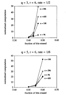
blocklengths. This is shown in Fig. 5 , which contains graphs of normalized computation versus fraction of bits erased for q = 3,
r = 6 and q = 5, r = 6. Here, the normalized computation is the
q = 3, r = 6, rate = 1/2 5 0 , El I 20 10 ~~ 0 0.30 n=3%
I
0.40 0.50 fraction of bits erasedq = 5, r = 6, rate = 1/6 6 0 , I 40 n=1%
i
- . 0.40 0.50 0.60fraction of bits erased
Fig. S. Normalized computation using the MNE algorithm, for two sets of ( q , r ) values and various values of n.
amount of computation divided by nq/r
+
1, the number of levels in the codeword tree with the root node. Both graphs seem to indicate that the cutoff point, where the average compu- tation starts to increase, occurs at roughly the same value of the fraction of bits erased, as n varies with q and r fixed. In otherwords, for fixed q and r , the number of decodable erasures
when using the MNE algorithm appears to increase linearly in
n. This behavior is expected, since the typical minimum distance of an ensemble of ( n , q, r ) low-density codes grows asymptoti-
cally linearly in n, for q 2 3 [ 5 ] , [6, p. 161. In addition, the cutoff becomes sharper with increasing n, in the following sense. For both graphs, at the first data point, normalized computation decreases with increasing n (for example, 1.18, 1.095, 1.0056, and 1.0050 for n equals 96, 198, 396 and 600, respectively, with
q = 3, r = 6). This represents a feasible operating point. At the second and third data points, normalized computation tends to increase with increasing n. This trend is somewhat obscured because trials were aborted if the computation reached 10000. Thus, normalized computation cannot exceed 10 000/(nq/r
+
1).What can we conclude about using the MNE algorithm at rates above R,, the computational cutoff rate for sequential decoding? Estimates of E ~the maximum erasure frequency ~ ,
handled by the MNE algorithm, are shown in Table I. The upper range is determined by the data point in Fig. 3 where the average computation first exceeds two times its minimum possi- ble value, n q / r
+
1. The lower range is given by the last data point with average computation less than 1.5(nq/r+
1). For example, for the (396,5,6) code, the relevant data points have 215 and 210 erasures out of 396 digits. The well-known formula of R , on a discrete memoryless channel [4, p. 2791 applied to the BEC yieldsTABLE I
CUTOFF POINTS FOR THE MNE ALGORITHM A N D STANDARD
SEQUENTIAL DECODING ON THE BEC Code Parameters Rate
n i k R EMNE ‘SD
-
lo00 3 10 0.7 0.245-0.251 0.2311 396 3 6 0.5 0.404-0.429 0.4142 396 4 6 0.333 0.480-0.505 0.5874 396 5 6 0.167 0.530-0.543 0.7818where E is the channel erasure probability and R , is measured
in bits. Inverting this formula yields the maximum erasure probability that sequential decoding can handle for a given code rate. Table I shows values of E ~ , , corresponding to the code
rates used in the simulations. For the (396,4,6) and (396,5,6) codes, sMVIM: for the MNE algorithm is significantly less than
E ~Thus, it seems that one cannot exceed ~ . R , using the MNE
algorithm with these values of q and r. The (396,3,6) code looks
more promising. Its value of E M N E nearly equals eSD.
Finally, for the (1000,3,10) code, s M N E is estimated to be greater than eSD. To interpret this, recall that the simulations were performed with fixed weight erasure patterns, not indepen- dent erasures. At n = 1000, with 245 erasures, normalized com- putation was 1.33. Extending this point proportionately out to
n = 5000 resulted in normalized computation equal to 1.0013. If the conjecture about a linearly increasing operating region is true, then it seems that an erasure frequency of 0.245 is within the operating region for all n (with q = 3, r = 10). This implies that for sufficiently large n , the MNE algorithm can handle independent erasures with erasure probability at least up to 0.245. This would exceed the performance of standard sequen- tial decoding, which has = 0.2311. Though this seems plau- sible, nevertheless a finite number of simulations cannot prove an asymptotic result.
Decoding errors occurred much less often than decoding failures. A decoding error occurs when the sequential decoder completes its search but outputs the wrong codeword. As de- fined here, a decoding failure occurs if a trial results in a decoding error or is aborted because of too much computation. Out of 31 069 trials used to generate the graphs in Fig. 3, only 8 resulted in decoding errors. Thus, if the MNE algorithm is used on a channel with feedback and retransmission capabilities, one can achieve decoding error rates several orders of magnitude smaller than p D F . However, the effective information rate would be lower than the code rate, because of retransmissions. For the results shown in Fig. 5, a significant number of decoding errors occurred when using the (96,3,6) and (198,3,6) codes. It seems one should avoid using blocklengths this small because, for the trials used to generate Fig. 5, none of the other codes had any decoding errors.
This discussion implicitly assumes that the codes used in the simulations are “typical” low-density codes. The assumption is reasonable in light of Gallager’s result that almost all the low-density codes in his ensemble have minimum distance greater than a single lower bound, Sq,n. In addition, for the binary
symmetric channel, simulation results obtained using two ran- domly chosen (396,5,6) low-density codes are found to be very close.
Given the extra work performed by the ordering algorithm, why doesn’t the MNE algorithm outperform standard sequential decoding in all cases? One feature that limits the SDR ap- proach, not encountered in standard sequential decoding, is that
codeword trees for low-density codes tend to grow more rapidly near the beginning than near the end. This happens regardless of the parity check ordering, as discussed in Section 11. Thus, the early part of the tree looks like a code with higher rate than the original code. This is a drawback, since the sequential decoder works well only at rates less than R,. However, the MNE
algorithm tends to push erased digits toward the end of the tree, and this helps the sequential decoder. The net result of these effects determines whether the overall performance is better than standard sequential decoding. Another limitation of the SDR approach is that the distance properties of low-density codes are probably not the best possible.
v.
T H E BINARY SYMMETRIC CHANNELResults for the binary symmetric channel (BSC) were not as promising ‘as for the BEC. Several ordering algorithms were implemented [9], but several problems were encountered. First, the same features that limit the SDR approach for the BEC apply to the BSC as well. The trees searched by the sequential decoder tend to grow more quickly near the root node than at later levels, and low-density codes may have suboptimal distance properties. Second, as discussed in Section 11, the trees used here are such that if the sequential decoder diverges from the correct path in the tree, it may not be able to detect its error for many levels. This is not a problem on the BEC because the unerased portion of a received message serves to eliminate from consideration many nodes in the tree. Since conventional se- quential decoders do not work well for this application on the BSC, a new sequential decoder [9] was designed, but the result- ing performance was still not good enough to approach the cutoff rate. Third, the BSC is, in a sense, the worst possible channel for SDR algorithms. Each digit at the channel output, taken by itself, is equally unreliable-unlike, for example, the BEC or the Gaussian noise channel. This makes it difficult to generate a good parity check ordering.
VI. CONCLUSION
Sequential decoding with reordering (SDR) algorithms were designed for the binary erasure and binary symmetric channels. For both channels, with respect to standard sequential decoding, relative performance improved with increasing code rate. For the erasure channel, simulations suggest that one can use rate 0.7 low-density codes to handle a higher probability of erasure than standard sequential decoding. A similar result did not hold for the errors channel.
For future work, one could consider different parity-check ordering algorithms. In addition, SDR algorithms could be gen- erated for other communication channels. For example, one could define f ( u ) = h ( P ( x , = OJy,)), where h is the entropy function. The resulting SDR algorithm could be used on chan- nels with real-valued outputs, such as the Gaussian noise chan- nel.
ACKNOWLEDGMENT
The authors thank the reviewers for their useful comments. REFERENCES
[I] G. C. Clark and J. B. Cain, Error-Correction Coding for Digital Communications. New York: Plenum Press, 1981.
[2] D. D . Falconer, “A hybrid sequential and algebraic decoding scheme,” Ph.D. dissert., Dept. of Elect. Eng., Massachusetts Inst. of Technol., Cambridge, MA, 1967.
IEEE TRANSACTIONS ON INFORMATION THEORY, VOL. 38, NO. 6, NOVEMBER 1992 1839
G. D. Forney, Jr., “Coset codes-Part 11: Binary lattices and related codes,” IEEE Trans. Inform. Theory, vol. 34, pp. 1152-1187, Sept. 1988.
R. G. Gallager, Information Theory and Reliable Communication. New York: Wiley, 1968.
-, “Low-density parity-check codes,” IRE Trans. Inform. The- ory, vol. IT-8, pp. 21-28, Jan. 1962.
-, Low-Density Parity-Check Codes. Cambridge, MA: M.I.T. Press, 1963.
I. M. Jacobs and E. R. Berlekamp, “A lower bound to the distribution of computation for sequential decoding,” ZEEE Trans. Inform. neory, vol. IT-13, pp. 167-174, Apr. 1967.
M. S. Pinsker, “On the complexity of decoding,” Probl. Inform. Trans. (translation of Probl. Pereduch. Inform.), vol. 1, pp. 84-86, Jan.-Mar. 1965.
B. Radosavljevic, “Sequential decoding with adaptive reordering of codeword trees,” M.S. thesis, Tech. Rep. UILU-ENG-90-2209, Coor. Sci. Lab., Univ. of Illinois, Urbana, IL, Mar. 1990. J. K. Wolf, “Efficient maximum likelihood decoding of linear blocks codes using a trellis,” IEEE Trans. Inform. Theory, vol. IT-24, pp. 76-80, Jan. 1978.
V. V. Zyablov and M. S. Pinsker, “Decoding complexity of low- density codes for transmission in a channel with erasures,” Probl. Inform. Trans. (translation of Probl. Pereduch. Inform.), vol. 10, pp.
10-21, Jan.-Mar. 1974.
-, “Estimation of the error-correction complexity for Gallager low-density codes,” Probl. Inform. Trans. (translation of Probl. Peredach. Inform.), vol. 11, pp. 18-28, Jan.-Mar. 1975.
The Lempel-Ziv Algorithm and Message Complexity
E. N. Gilbert, Fellow, IEEE, and T. T. Kadota, Fellow, IEEE Abstract-Data compression has been suggested as a non-parametric way of discriminating between message sources (e.g., a complex noise message should compress less than a more redundant signal message). Compressions obtained from a Lempel-Ziv algorithm for relatively short messages, such as those encountered in practice, are examined. The intuitive notion of message complexity has less connection with compression than one might expect from known asymptotic results about infinite messages. Nevertheless, discrimination by compression remains an interesting possibility.
Index Terms-Lempel-Ziv parsing, data compression, nonparametric discrimination.
I. INTRODUCTION
A discrimination question asks which of two possible sources (e.g., signal or noise) produced a received message. If good probabilistic descriptions of the sources were known, a likeli- hood ratio might decide. Often the sources are not well under- stood and nonparametric methods are needed. If the two sources differ in redundancy, then data compression may be used ([1]-[3]). Thus, redundant signal messages will compress more than non-redundant noise messages. Here, we examine Lempel-Ziv compression for properties that may be useful in discriminating binary sources.
There are several Lempel-Ziv algorithms. The one we study scans the message digits in order and creates a new word Manuscript received October 7, 1991; revised March 3, 1992. This work was presented in part at the IEEE International Symposium on Information Theory, Budapest, Hungary, June 24-28, 1991.
The authors are with AT & T Bell Laboratories, 600 Mountain Av- enue, Murray Hill, NJ 07974.
IEEE Log Number 9201221.
whenever the current block of unparsed digits differs from all words already found. Suppose the first m words from the mes- sage contain a total of s, digits. Then, s, will tend to be large for repetitious or redundant messages. As m goes to infinity, a
well-known result ([2], [4]) shows that s, increases like (mlogm)/H, where H is the entropy of the source. Thus,
sources with different entropies could be perfectly discriminated by parsing infinite messages.
Long messages are not available in real discrimination prob- lems; moreover the asymptotic formula is found to be inaccurate until m is very large indeed. For these reasons, we avoid asymptotic results and concentrate on finite values of m. Even small values like m = 3 or 4 provide interesting counterexam- ples to show that properties holding for large m need not hold in general. If m is small, and especially for highly redundant sources, compression is found to be only very roughly related to the intuitive notion of message complexity. For instance, two messages that are just reversals of one another may compress very differently (Section V). However, compression does give a basis for discriminating. The main analytical results follow from a useful identity (1) that enumerates parsed messages.
11. ENUMERATION
A list L , of all possible messages composed of m parsed words will be a basic tool ( L , lists six messages 0,OO; 0,Ol; 0,l; 1,O; 1,lO; 1,111. In principle, any probability related to the first m words (e.g., the probability distribution of s), from any known source can be computed by evaluating the probability of each message in L,. Since L , contains (m
+
l)! messages [5], such computations become impractical with large m but here, with smaller m, they give some insight. Memoryless sources, consid- ered in Section 111, allow simplifications for larger m.An inductive procedure constructs L,. Suppose L,;.., L , -
,
are known. Construct L , as follows. One message in L , is O,OO,OOO,
... with m(m
+
1)/2 digits, all zeros. Another message has all ones. Other messages have a number k 2 0 of words beginning 0 and m - k 2 0 words beginning 1. The first word beginning with 0 is 0 itself. Any remaining words beginning with 0 are, in parsing order, the words A , , A , , ... of one member ofL k _ with an extra 0 added as prefix to each word. Similarly, the
words beginning with 1 will be 1,1 B , , 1 B,,
...
where B , , B,,...
are the words of a parsed message in L m - k - 1. Thus, with m = 5 and k = 2, the choices 1 from L , and 0,Ol from L , determine the words 0,Ol and 1,10,101. These two parsings can be inter- leaved, keeping the words OA, and lBJ in the same order, toproduce parsed messages like 1,10,0,101,01. In general, for given m, k , and given choices from L,_ and L ,
-,-
1, there are(T
)
possible interleavings.One can easily verify that this procedure lists only Lempel-Ziv parsings. That is, 1) the words of each parsing are distinct and 2 )
each parsing contains, as words, all proper prefixes of each of its words. Conversely, every Lempel-Ziv parsing into m words is found by this procedure.
Counting the choices that arise in this procedure leads to a count of the number f(m, i, j ) of parsings with m words, z zeros, and j ones. The result is stated most simply in terms of the generating function F,(x, y ) =