RECOGNITION AND CLASSIFICATION OF
HUMAN ACTIVITIES USING WEARABLE
SENSORS
a thesis
submitted to the department of electrical and
electronics engineering
and the graduate school of engineering and science
of bilkent university
in partial fulfillment of the requirements
for the degree of
master of science
By
Aras Yurtman
September 2012
I certify that I have read this thesis and that in my opinion it is fully adequate, in scope and in quality, as a thesis for the degree of Master of Science.
Prof. Dr. Billur Barshan (Advisor)
I certify that I have read this thesis and that in my opinion it is fully adequate, in scope and in quality, as a thesis for the degree of Master of Science.
Assoc. Prof. Dr. Nail Akar
I certify that I have read this thesis and that in my opinion it is fully adequate, in scope and in quality, as a thesis for the degree of Master of Science.
Assist. Prof. Dr. Beh¸cet U˘gur T¨oreyin
Approved for the Graduate School of Engineering and Science:
Prof. Dr. Levent Onural Director of the Graduate School
ABSTRACT
RECOGNITION AND CLASSIFICATION OF HUMAN
ACTIVITIES USING WEARABLE SENSORS
Aras Yurtman
M.S. in Electrical and Electronics Engineering Supervisor: Prof. Dr. Billur Barshan
September 2012
We address the problem of detecting and classifying human activities using two different types of wearable sensors. In the first part of the thesis, a com-parative study on the different techniques of classifying human activities using tag-based radio-frequency (RF) localization is provided. Position data of multiple RF tags worn on the human body are acquired asynchronously and non-uniformly. Curves fitted to the data are re-sampled uniformly and then segmented. The effect of varying the relevant system parameters on the system accuracy is investigated. Various curve-fitting, segmentation, and classification techniques are compared and the combination resulting in the best performance is presented. The clas-sifiers are validated through the use of two different cross-validation methods. For the complete classification problem with 11 classes, the proposed system demonstrates an average classification error of 8.67% and 21.30% for 5-fold and subject-based leave-one-out (L1O) cross validation, respectively. When the num-ber of classes is reduced to five by omitting the transition classes, these errors become 1.12% and 6.52%. The system demonstrates acceptable classification per-formance despite that tag-based RF localization does not provide very accurate position measurements.
In the second part, data acquired from five sensory units worn on the human body, each containing a tri-axial accelerometer, a gyroscope, and a magnetometer, during 19 different human activities are used to calculate subject and inter-activity variations in the data with different methods. Absolute, Euclidean, and dynamic time-warping (DTW) distances are used to assess the similarity of the signals. The comparisons are made using time-domain data and feature vectors. Different normalization methods are used and compared. The “best” subject is defined and identified according to his/her average distance to the other subjects.
iv
Based on one of the similarity criteria proposed here, an autonomous system that detects and evaluates physical therapy exercises using inertial sensors and magnetometers is developed. An algorithm that detects all the occurrences of one or more template signals (exercise movements) in a long signal (physical therapy session) while allowing some distortion is proposed based on DTW. The algorithm classifies the executions in one of the exercises and evaluates them as correct/incorrect, identifying the error type if there is any. To evaluate the performance of the algorithm in physical therapy, a dataset consisting of one template execution and ten test executions of each of the three execution types of eight exercise movements performed by five subjects is recorded, having totally 120 and 1,200 exercise executions in the training and test sets, respectively, as well as many idle time intervals in the test signals. The proposed algorithm detects 1,125 executions in the whole test set. 8.58% of the executions are missed and 4.91% of the idle intervals are incorrectly detected as an execution. The accuracy is 93.46% for exercise classification and 88.65% for both exercise and execution type classification. The proposed system may be used to both estimate the intensity of the physical therapy session and evaluate the executions to provide feedback to the patient and the specialist.
Keywords: radio-frequency localization, radio-frequency identification, human activity recognition, pattern recognition, classification, feature extraction, feature reduction, principal components analysis, linear discriminant analysis, P -fold cross-validation, leave-one-out cross-validation, absolute distance, Euclidean distance, dynamic time warping, subsequence dynamic time warping, dynamic programming, normalization, inertial sensors, accelerometers, gyroscopes, mag-netometers, pattern search, movement detection, physical therapy.
¨
OZET
G˙IY˙ILEB˙IL˙IR DUYUCULARLA ˙INSAN
AKT˙IV˙ITELER˙IN˙IN ALGILANMASI VE
SINIFLANDIRILMASI
Aras Yurtman
Elektrik ve Elektronik M¨uhendisli˘gi, Y¨uksek Lisans
Tez Y¨oneticisi: Prof. Dr. Billur Barshan
Eyl¨ul 2012
Farklı t¨urde giyilebilir algılayıcılar kullanarak insan aktivitelerinin sezimi ve
sınıflandırılması ele alınmaktadır. Tezin ilk b¨ol¨um¨unde, etiket tabanlı, radyo
frekansına dayalı bir konumlama sistemi ile insan aktivitesi tanımada ¸ce¸sitli
y¨ontemlerin kullanımı kar¸sıla¸stırmalı olarak sunulmu¸stur. ˙Insan bedeninin farklı
b¨olgelerine yerle¸stirilen etiketlerin konumları, e¸szamansız ve farklı aralıklarla
¨
orneklenmi¸s olarak elde edilmektedir. Bu verilere uyarlanan e˘griler, d¨uzg¨un
¨
orneklenmi¸s ve b¨ol¨utlenmi¸stir. ˙Ilgili sistem parametrelerinin sistem ba¸sarımına
etkisi incelenmi¸stir. C¸ e¸sitli e˘gri uyarlama, b¨ol¨utleme ve sınıflandırma y¨ontemleri
kar¸sıla¸stırılmı¸s ve en iyi ba¸sarımı veren katı¸sım sunulmu¸stur. Sınıflandırıcılar,
iki farklı ba˘gımsız ge¸cerlilik sınaması y¨ontemiyle de˘gerlendirilmi¸stir. 11 sınıftan
olu¸san sınıflandırma probleminde, sırasıyla P -b¨olmeli ve birini dı¸sarıda bırak
ba˘gımsız ge¸cerlilik sınamaları kullanıldı˘gında ortalama sınıflandırma hataları
%8.67 ve %21.30 olarak elde edilmi¸stir. Ge¸ci¸s sınıfları dı¸sarıda bırakılarak
elde edilen be¸s sınıflı sınıflandırma probleminde ise, bu hatalar %1.12 ve
%6.52’ye d¨u¸smektedir. Etiket-tabanlı konumlama sistemlerinin ¸cok hassas
konum ¨ol¸c¨umleri sa˘glamamasına kar¸sın sonu¸clar, sistemin kabul edilebilir bir
sınıflandırma ba¸sarımı sundu˘gunu g¨ostermektedir.
˙Ikinci b¨ol¨umde, insan bedeninin be¸s noktasına yerle¸stirilmi¸s, her biri ¨u¸c
eksenli ivme¨ol¸cer, d¨on¨u¨ol¸cer ve manyetometre i¸ceren be¸s duyucu ¨unitesinden
19 farklı g¨unl¨uk aktivite sırasında elde edilen veriler, katılımcılar arası ve
aktiviteler arası farklılıkları ¸ce¸sitli y¨ontemlerle hesaplamak i¸cin kullanılmı¸stır.
˙I¸saretlerin kar¸sıla¸stırılması i¸cin mutlak, ¨Oklit ve dinamik zaman b¨ukmesi (DZB)
uzaklıkları kullanılmı¸stır. Kar¸sıla¸stırmalar, zaman b¨olgesindeki veri ve ¨oznitelik
vi
ve kar¸sıla¸stırılmı¸stır. “En iyi” katılımcı, di˘ger katılımcılara olan ortalama
uzaklı˘ga dayalı olarak tanımlanmı¸s ve saptanmı¸stır. Bu kısımda ¨onerilen
benzerlik ¨ol¸c¨utlerinden biri se¸cilerek, eylemsizlik duyucuları ve manyetometreler
kullanılarak fizik tedavi egzersizlerini sezen ve de˘gerlendiren ¨ozerk bir sistem
geli¸stirilmi¸stir. DZB y¨ontemine dayanarak belirli ¨ol¸c¨ude bozuluma izin vererek,
uzun bir i¸saretin (fizik tedavi seansı) i¸cinde bir ya da birden fazla ¸sablon i¸saretin
(fizik tedavi hareketkeri) b¨ut¨un olageli¸slerini sezen bir algoritma ¨one s¨ur¨ulm¨u¸st¨ur.
Bu algoritma, y¨ur¨ut¨umleri egzersiz hareketlerinden birisi olarak sınıflandırmakta,
do˘gru/yanlı¸s olarak de˘gerlendirmekte ve e˘ger varsa yapılan hatanın t¨ur¨un¨u
belirtmektedir. Algoritmanın fizik tedavideki ba¸sarımını belirlemek i¸cin, be¸s
katılımcı tarafından y¨ur¨ut¨ulen sekiz egzersiz hareketinin ¨u¸c farklı yapılı¸s bi¸ciminin
her biri i¸cin bir ¸sablon ve on test y¨ur¨ut¨um¨unden olu¸san ve b¨oylece e˘gitim
ve test veri k¨umelerinde sırasıyla 120 ve 1,200 egzersiz y¨ur¨ut¨um¨u ile test
i¸saretlerinde bir¸cok bo¸s zaman aralı˘gı i¸ceren bir veri k¨umesi kaydedilmi¸stir. ¨One
s¨ur¨ulen algoritma, b¨ut¨un test k¨umesinde 1,125 y¨ur¨ut¨um sezmi¸stir. Y¨ur¨ut¨umlerin
%8.58’i sezilememi¸s, bo¸s aralıkların %4.91’i yanlı¸slıkla y¨ur¨ut¨um olarak sezilmi¸stir.
Ba¸sarım, egzersiz ayırt etmede %93.46, hem egzersiz hem de yapılı¸s ¸sekli ayırt
etmede %88.65’tir. Geli¸stirilen sistem, hem fizik tedavi seansının yo˘gunlu˘gunu
kestirmek i¸cin, hem de egzersiz y¨ur¨ut¨umlerini de˘gerlendirerek hastaya ve uzmana
geribildirim vermek i¸cin kullanılabilir.
Anahtar s¨ozc¨ukler : radyo-frekanslı konumlama, radyo-frekanslı tanımlama,
in-san aktivitesi tanıma, ¨or¨unt¨u tanıma, sınıflandırma, ¨oznitelik ¸cıkarma, ¨oznitelik
indirgeme, ana bile¸senler ¸c¨oz¨umlemesi, do˘grusal ayırta¸c ¸c¨oz¨umlemesi, P -b¨olmeli
ba˘gımsız ge¸cerlilik sınaması, birini dı¸sarıda bırak ba˘gımsız ge¸cerlilik sınaması,
mutlak uzaklık, ¨Oklit uzaklı˘gı, dinamik zaman b¨ukmesi, altdizi dinamik zaman
b¨ukmesi, dinamik programlama, d¨uzgeleme, eylemsizlik duyucuları,
Acknowledgement
I would like to express my gratitude to my supervisor Prof. Dr. Billur Barshan for her support in the development of this thesis.
I would like to thank Assoc. Prof. Dr. ˙Ilknur Tu˘gcu for sharing the literature
and invaluable assistance in the field of physical therapy.
I would also like to thank Assoc. Prof. Dr. Nail Akar and
Assist. Prof. Dr. Beh¸cet U˘gur T¨oreyin for accepting to read and review
Contents
1 Introduction 1
1.1 Approaches in Activity Recognition . . . 1
1.1.1 Activity Recognition Using Visual Sensors . . . 2
1.1.2 Activity Recognition Using Radio-Frequency Localization . 2
1.1.3 Activity Recognition Using Inertial Sensors . . . 6
CONTENTS ix
2 Human Activity Recognition Using Tag-Based Radio-Frequency
Localization 11
2.1 The System Details . . . 12
2.2 Pre-processing of the Data . . . 17
2.2.1 Curve-Fitting . . . 17
2.2.2 Segmentation . . . 20
2.3 Feature Extraction and Reduction . . . 21
2.3.1 Feature Extraction . . . 21
2.3.2 Feature Reduction . . . 21
2.4 Classification . . . 22
2.5 Performance Evaluation through Cross Validation . . . 23
2.6 Experimental Results . . . 24
2.6.1 Effect of the Sampling Frequency (fs) . . . 29
2.6.2 Effect of the Segment Duration (frm dur) . . . 30
2.6.3 Effect of the Curve-Fitting Algorithm . . . 31
2.6.4 Effect of the Prior Probabilities . . . 32
2.6.5 Effect of Feature Reduction . . . 33
CONTENTS x
3 Investigation of Personal Variations in Activity Recognition
Us-ing Inertial Sensors and Magnetometers 37
3.1 Introduction and Related Work . . . 37
3.2 Dataset . . . 39
3.3 Distance Measures . . . 41
3.4 Normalization . . . 42
3.5 Inter- and Intra-Subject Variations in Activity Recognition Using Inertial Sensors and Magnetometers . . . 44
3.5.1 Identifying the ‘Best’ Subjects . . . 44
3.5.2 Average Inter-Subject Distance per Activity . . . 48
3.5.3 Average Mean and Standard Deviation of Inter-Activity Distances for Each Subject, Unit, Sensor . . . 50
3.6 Discussion . . . 55
CONTENTS xi
4 Automated Evaluation of Physical Therapy Exercises Using
Multi-Template Dynamic Time-Warping on Wearable Sensor
Signals 59
4.1 Related Work . . . 63
4.2 Modifications to the DTW Algorithm . . . 67
4.2.1 Single-Template Multi-Match DTW (STMM-DTW) . . . . 69
4.2.2 Multi-Template Multi-Match DTW (MTMM-DTW) . . . 71
4.3 Experiments and Results . . . 74
4.3.1 Physical Setup . . . 74
4.3.2 Exercises . . . 75
4.3.3 Experiments . . . 78
4.3.4 Movement Detection and Classification . . . 82
4.3.5 Experimental Results . . . 83
4.3.6 Computational Complexity . . . 91
4.4 Conclusion . . . 92
5 Conclusion and Future Work 94 5.1 Conclusion . . . 94
5.2 Future Work . . . 98
A Dynamic Time Warping 100 A.1 Multi-Dimensional Signals . . . 103
A.2 Local Weights . . . 103
List of Figures
1.1 Examples of RFID tags. . . 4
1.2 Xsens MTx and 3DM-GX2 sensor units. . . 7
1.3 Miniature inertial sensor units worn on the body. . . 7
2.1 Ubisense hardware components. . . 13
2.2 Sample rows of the original dataset. . . 15
2.3 The positions of tag 1 and tag 3 in the first experiment of the first subject as 3-D curves along time. . . 16
2.4 The three curve-fitting methods applied to synthetic position data. 18 2.5 The x position of tag 4 in the fifth experiment of the fifth subject. 19 2.6 Effect of the sampling frequency. . . 29
2.7 Effect of the segment duration. . . 30
2.8 Effect of the curve fitting method. . . 31
2.9 Effect of the prior probabilities. . . 32
2.10 Effect of feature reduction with LDA and PCA. . . 34
LIST OF FIGURES xiii
3.2 Average distance of each subject to the others in terms of different
distance measures for different normalization methods. . . 47
3.3 Average distance between all distinct subject pairs for each activity. 49
3.4 Average mean and standard deviation of inter-activity distances
for each subject in terms of three different distance functions. . . 52
3.5 Average mean and standard deviation of inter-activity distances
for each unit in terms of three different distance functions. . . 54
3.6 Average mean and standard deviation of inter-activity distances
for each sensor in terms of three different distance functions. . . . 56
4.1 Sensor placement on the human body. . . 76
4.2 Recording of the templates and the experiment for exercise 1
per-formed by subject 3. . . 80
4.3 Detection and classification of exercise executions in all of the 8
List of Tables
2.1 The average probability of error of each classifier with the
corre-sponding parameter values. . . 26
2.2 Cumulative confusion matrices for classifier 6 for the 11-class
prob-lem. . . 27
2.3 Cumulative confusion matrices for classifier 6 for the 5-class problem. 28
4.1 Physical properties of the subjects who performed the experiments. 81
4.2 The results summarized for all of the 5 subjects. . . 84
4.3 The results summarized for all of the 8 exercises. . . 85
4.4 Cumulative confusion matrix that contains the three execution
types of all of the 8 exercises for all of the 5 subjects. . . 89
4.5 Cumulative confusion matrix of all of the 8 exercises for all of the
Chapter 1
Introduction
With rapidly developing technology, devices such as personal digital assistants (PDAs), smart phones, and tablet computers have made their way to our daily lives. It is now becoming essential for such devices to recognize and interpret human behavior correctly in real time. One aspect of this type of context-aware systems is the recognition and monitoring of activities of daily living such as sitting, standing, lying down, walking, ascending/descending stairs, and most importantly, falling.
1.1
Approaches in Activity Recognition
There exist several different approaches for the recognition of human activities in the literature [1]. The most common three approaches are based on computer vision, radio-frequency localization systems, and inertial sensors. Earlier work in this area is summarized below.
1.1.1
Activity Recognition Using Visual Sensors
A large number of studies employ vision-based systems with multiple video cam-eras mounted in the environment to recognize the activities performed by a per-son [2–5]. In many of these studies, points of interest on the human body are pre-identified by placing special, visible markers such as light-emitting diodes (LEDs) at those points and the positions of the markers are recorded by
cam-eras [6]. For example, Kaluˇza et al. [7] considered a total of six activities including
falls using the Smart infrared motion capture system. The attributes they used are the coordinates of the body parts in different coordinate systems and the angles between adjacent body parts. In Luˇstrek et al. [8], walking anomalies, such as limping, dizziness, and hemiplegia are detected using the same system. Camera systems obviously interfere with privacy since they capture additional information that is not needed by the system but that may easily be exploited with a simple modification on the software. Hence, people act unnaturally and feel uncomfortable when camera systems are used, especially in private places. Other disadvantages of vision-based systems are the high computational cost of processing images and videos, correspondence and shadowing problems, the need for camera calibration, and inoperability in the dark. When multiple cameras are employed, several 2-D projections of the 3-D scene have to be combined. More-over, this approach imposes restrictions on the mobility of the person since the system operates only in the limited environment monitored by the cameras.
1.1.2
Activity Recognition Using Radio-Frequency
Local-ization
Rather than monitoring human activities from a distance or remotely, we believe that “activity can best be measured where it occurs” as stated in [9]. Unlike the first approach utilizing visual sensors, the use of inertial sensors and the radio-frequency (RF) localization-based approach directly acquire the motion data and position data in 3-D, respectively. In the RF localization technique, the 3-D
positions of the RF tags worn on different parts of the body are estimated1.
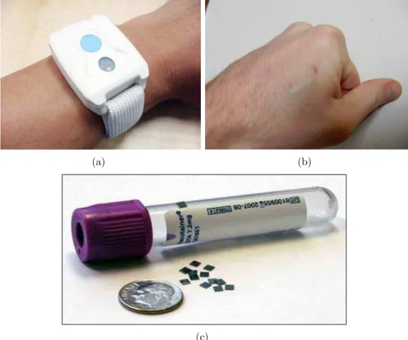
Multiple antennas called readers are mounted in the environment that detect the relative positions of small devices called RF tags (Figure 1.1). Each tag emits RF pulses containing its unique ID for identification and localization. Active RF tags have internal power sources (batteries) to transmit RF pulses, whereas passive tags do not contain a power source and rely on the energy of the waves transmitted by the readers [11]. Passive RF tags are small stickers similar to RFID tags that can be as small as 2 mm × 2 mm in size (Figure 1.1(c)), whereas active RF tags are much larger than the passive ones (Figure 1.1(a)). RF tags are very inexpensive and lightweight, and thus comfortable to use on the human body [12]. Unlike bar codes, the tag does not need to be within the line of sight of the reader and may be embedded in the tracked object or even buried under the skin (Figure 1.1(b)).
The operating range of most RF readers is not more than 10 m [13]. In uncluttered, open environments, typical localization accuracy is about 15 cm across 95% of the readings [14]. Since each tag must be detected by multiple readers for localization, this method cannot be used in large areas because in that case, numerous readers are needed, which would be too costly. On the other hand, the number of RF tags that can be worn on the body is limited. In systems that use active tags, the pulses transmitted by the tags may interfere, whereas in systems that use passive tags, it becomes difficult for the system to distinguish the tags that are close together.
RFID technology is a very valuable tool in a variety of applications involv-ing the automatic detection, identification, localization, and trackinvolv-ing of persons, animals, vehicles, baggage, and goods [15]. RFID systems are used for general
1Radio-Frequency Identification (RFID)is a technique involving the detection and
identifica-tionof tags (deciding which tags exist in the environment), whereas in RF localization, the tags are both identified and localized. The tags are called “RFID tags” in the former system and “RF tags” in the latter although they can be identical in some cases [10, 11]. In this thesis, the tags used for localization are not the same as RFID tags, hence will be called “RF tags.” How-ever, in some texts, the term “RFID localization” is used instead of RF localization because there are systems estimating the positions of RFID tags that are designed for identification only [10].
(a) (b)
(c)
Figure 1.1: Examples of RFID tags. (a) an active RFID tag worn as
a bracelet (Syris sytag245-tm, reprinted from http://blog.aztronics.com/ ?p=45), (b) an RFID tag buried under the skin (An RFID Body Mod Most Curious, Ization Labs, reprinted from http://izationlabs.com/2009/ 12/22/a-body-mod-most-curious/), (c) tiny RFID tags of size 2 mm × 2 mm (Chip-size Passive RFID Tag, Health Care News, RFID Journal, reprinted from http://www.rfidjournal.com/imagecatalogue/imageview/ 5866/?RefererURL=/article/view/4585).
transport logistics, toll collection from vehicles and contactless payment, tracking of parcels and baggage, and to avoid theft of the items sold in stores or super-markets. With the use of RFID tags, assembly lines and inventories in the supply chain can be tracked more efficiently and products become harder to falsify. This is particularly important for the pharmaceutical industry with increasing anti-counterfeit measures. In the identification and tracking of animals, RFID tags are used for tracking pets, farm animals, and rare animal species such as pandas. They are used on contactless identity cards for access management and control of hospitals, libraries, museums, schools and universities, and restricted zones. Ma-chine readable identification and travel documents such as biometric passports that contain RFID tags are becoming very common. RFID tags are also used for key identification in vehicles, for locking/unlocking vehicles from a distance, ticketing of mass events or public transport, and transponder timing of sporting events.
Besides the above uses, RFID systems are also suitable for indoor localization and mapping [16]. Reference [17] analyzes whether the use of RFID technology in the field of robotics can improve the localization of mobile robots and persons in their environment and determines the computational requirements. In [18], many RFID tags are placed on the floor in a grid configuration at known positions and a robot localizes itself by detecting the tags using its antenna. To resolve the issues concerning security and privacy of RFID systems, reference [19] proposes an authentication protocol based on RFID tags.
There are many studies involving activity recognition using RFID; however, they are not based on RF localization. In the earlier work on human activity recognition using RFID technology, activities of daily living are mostly inferred based on the interactions of a person with the objects in its environment. RFID antennas are worn on the body usually in the form of gloves or bracelets, and RFID tags are fixed to the objects in the environment such as equipment, tools, furniture, or doors (or vice versa). Then, the position of the subject and the activity s/he is performing is estimated from the tag readings in consequence of body-object interactions. The main limitation of these systems is that they provide activity information only when the subject interacts with one of the
tagged objects in its environment. Thus, the only recognizable activities are those that involve these objects. This type of approach is followed in [20–24]. Similarly, in [25], the authors employ RFID sensor networks based on wireless identification and sensing platforms (WISPs) that combine passive UHF RFID technology with traditional sensors. Everyday objects are tagged with WISPs to detect when they are in use, and a simple hidden Markov model (HMM) is used to convert object traces into high-level daily activities. In [26], a dynamic Bayesian network model is presented that combines RFID and video data to jointly infer the most likely household activity and object labels. Reference [27] combines data from RFID tag readers and accelerometers to recognize ten housekeeping activities with higher accuracy. A multi-agent system for fall and disability detection of the elderly living alone is presented in [28], based on the commercially available Ubisense smart space platform [14]. On the other hand, in (Chapter 2 of) this thesis, human activities are recognized by using an RF localization system, where the 3-D position estimations of the RF tags are used. This technique does not require any object interactions. Furthermore, a new approach based on curve-fitting is applied to the non-uniform and asynchronous position measurements of the RF tags to segment them and extract their features. This approach also solves the problem of missing data that is encountered in RF localization systems.
1.1.3
Activity Recognition Using Inertial Sensors
The third approach utilizes miniature inertial sensors whose size, weight, and cost have decreased considerably during the last two decades. The availability of lower cost, medium performance inertial sensor units has opened up new possibilities for their use. In this approach, several sensor units are worn on different parts of the body. These units usually contain gyroscopes and accelerometers, and sometimes, magnetometers in addition. Some of these devices are sensitive around a single axis whereas others are multi-axial (usually two- or three-axial). Two examples are shown in Figure 1.2 and a wearable system is illustrated in Figure 1.3.
Inertial sensors do not directly provide linear or angular position informa-tion. Gyroscopes provide angular rate information around an axis of sensitivity,
(a) (b)
Figure 1.2: (a) Xsens MTx [29] and (b) 3DM-GX2 [30] sensor units.
Figure 1.3: Miniature inertial sensor units worn on the body (reprinted from http://www.xsens.com/en/movement-science/xbus-kit).
whereas accelerometers provide linear or angular velocity rate information. These rate outputs need to be integrated once or twice to obtain the linear/angular po-sition. Thus, even very small errors in the rate information provided by inertial sensors cause an unbounded growth in the error of integrated measurements.
The acquired measurements are either collected and processed in a battery-powered system such as a cellular phone, or wirelessly transmitted to a computer to be processed. Detailed literature surveys on activity recognition using inertial sensors can be found in [31–35]. In the earlier work on human activity recognition, the utilization of inertial sensors [35–38] is also considered. Although this method results in accurate classification, wearing the sensors and the processing unit on the body may not always be comfortable or even acceptable despite how small and lightweight they have become. People may forget or neglect to wear these devices. Furthermore, this approach has certain limitations: Although it is demonstrated that it is possible to recognize activities with high accuracy (typically above 95%), the same is not true for human localization because of the drift problem associated with inertial sensors [39,40]. In [39], it is considered to exploit activity cues to improve the erroneous position estimates provided by inertial sensors and have achieved significantly better accuracies in localization when performed simultaneously with activity recognition.
In many studies on activity recognition with wearable inertial sensors, it is observed that the classification accuracy decreases significantly when the activi-ties of a subject are classified using the classifiers trained with the data of other subjects [35]. However, the reason is not investigated so far. For this purpose, us-ing the previous activity recognition dataset [35], inter-subject and intra-subject variations in the data are investigated in detail in Chapter 3. The signals are normalized with various methods. To compare signals, different distance mea-sures are used. Based on the results, the subject that performs the activities in the best way is also identified.
1.2
Application
of
Activity
Recognition
in
Physical Therapy
A different aspect of activity recognition may be very useful in detecting and evaluating exercise movements in the physical therapy field. The patients often perform the prescribed exercise movements in a hospital or a rehabilitation center for a while and they continue exercising at home, where they receive no feedback about how correctly they perform [41]. In addition, while exercising under the supervision of a specialist, it is common that the patients receive poor feedback due to the number of personnel being insufficient, the difficulty of tracking several patients at the same time, and/or subjective feedback due to negligence of the specialists and the lack of systematic rules for many exercises [42, 43]. For this purpose, it would be very useful and valuable if the individual exercise movements can be evaluated automatically by an intelligent system utilizing wearable sensors, as done in Chapter 4 in this thesis. For example, wearable miniature inertial sensors or an RF localization system with RF tags placed on the body can be used, both of which are much less expensive and highly portable compared to medical devices such as biofeedback devices [44]. In addition, both systems are easier to be placed on the body by the patient himself compared to tight garments containing strain sensors, which are used, for example, in reference [45].
In (Chapter 4 of) this thesis, we use one of the similarity criteria proposed in Chapter 3 to detect and evaluate the executions of physical therapy exercises automatically using wearable sensing units. An algorithm that detects all the occurrences of one or more template signals (exercise movements) in a long signal (physical therapy session) while allowing some distortion is proposed based on DTW. The algorithm classifies the executions in one of the exercises and evaluates them as correct/incorrect, identifying the error type if there is any. The developed system also estimates the number of (correct or all) executions, providing feedback about not only the correctness of the executions, but also the effectiveness or intensity of physical therapy sessions.
The organization of this thesis is as follows: In Chapter 2, human activities are classified using an RF localization system and various classification meth-ods. Variations in inertial sensor data of human activities performed by different subjects are examined in Chapter 3 and three similarity criteria are proposed. In Chapter 4, a system that detects and evaluates physical therapy exercises by using a novel algorithm applied to inertial sensor and magnetometer data is pre-sented based on one of the similarity criteria proposed in Chapter 3. Finally, in Chapter 5, conclusions are drawn and directions for future work are provided.
Chapter 2
Human Activity Recognition
Using Tag-Based
Radio-Frequency Localization
In this chapter, human activities are classified using an RF localization system. The work presented in this chapter is an extension of the study in reference [46]. An important issue in most RF systems is that the system measures the tag positions asynchronously and non-uniformly at different, arbitrary time instants. In other words, whenever the readers receive a pulse transmitted by an RF tag, the system records its relative position along the x, y, z axes as well as a unique timestamp and its unique ID. Although each tag transmits pulses periodically, tags cannot be synchronized since their pulses must not interfere with each other and thus the locations of the tags are sampled at different time instants. Further-more, the readers sometimes cannot detect the pulses due to low signal-to-noise ratio (SNR), interference, or occlusion. Under these circumstances, localization accuracy may drop significantly. The detection ratio of a tag increases when it is close to the antennas and decreases when it is near conductive objects. Thus, it is not possible to treat the raw measurements as ordinary position vectors sampled at a constant rate in time.
In this study, we consider a broad set of daily activity types (11 activities) and recognize these activities with high accuracy without having to take into account the interaction of a person with the objects in its environment. We only keep track of the position data of four RF tags worn on different parts of the body, acquired by the Ubisense platform [14]. In the data pre-processing stage, we propose a method to put the dataset in uniformly and synchronously sampled form. After feature reduction in two different ways, we compare several classifiers through the use of P -fold and subject-based leave-one-out (L1O) cross-validation techniques. The variation of the relevant system parameters on the classification performance is investigated.
In Section 2.1, details of the experimental setup and the dataset are provided. Section 2.2 describes pprocessing of the dataset. Feature extraction and re-duction is the topic of Section 2.3. Classifiers used for activity recognition are listed in Section 2.4. Section 2.5 describes the performance evaluation of the classifiers through the use of two cross-validation techniques. In Section 2.6, ex-perimental results are presented and interpreted. Lastly, conclusions are drawn in Section 2.7.
2.1
The System Details
The human activity recognition system employed in this study employs four active RF tags worn on different parts of the body, whose relative positions along the three axes are detected by a computer or a simple microcontroller via four RF antennas mounted in the environment (see Figure 2.1) [47]. The four RF tags are positioned on the left ankle (tag 1), right ankle (tag 2), chest (tag 3) and the belt (tag 4).
The 3-D position data of the four RF tags worn by a subject are measured over time while s/he is performing a fixed sequence of predetermined activities. The operating range of the system is about 46 m. Although each tag transmits a pulse every 0.1 s, the readers may miss some of the pulses (due to occlusion, low SNR at large distances, etc.) and therefore, the data acquisition rate is not
Figure 2.1: Ubisense hardware components [14].
constant. However, the average detection rate does not vary too much and is about 9 Hz most of the time.
The 11 activity types are numbered as follows: (1): walking, (2): falling, (3): lying down, (4): lying, (5): sitting down, (6): sitting, (7): standing up from lying, (8): on all fours, (9): sitting on the ground, (10): standing up from sitting, (11): standing up from sitting on the ground.
Each subject performs a sequence of activities referred as an “experiment” in this chapter. Each experiment consists of the following sequence of activities with different but similar durations:
walking—sitting down—sitting—standing up from sitting— walking—falling—lying—standing up from lying—walking— lying down—lying—standing up from lying—walking—falling— lying—standing up from lying—walking—sitting down—sitting— sitting on the ground—standing up from sitting on the ground— walking—lying down—lying—standing up from lying—walking— lying down—on all fours—lying—standing up from lying—walking
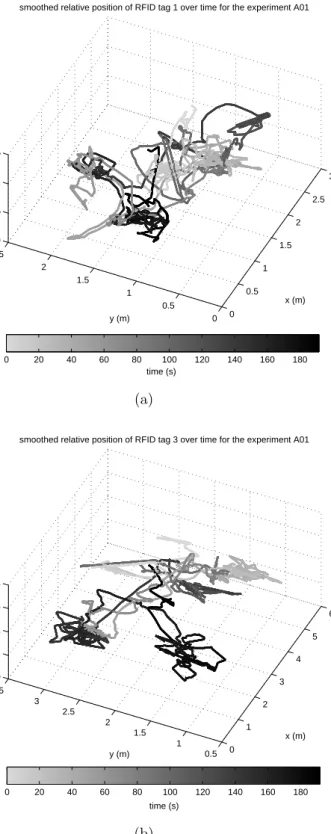
there is a total of 5 × 5 = 25 experiments of the same scenario. The dataset described above and used in this study is entitled “Localization Data for Person Activity Data Set” and is publicly available at the University of California, Irvine Machine Learning Repository [47]. The dataset is an extremely long but simple-structured 2-D array of size 164, 860 × 8 (see Figure 2.2 for sample rows). Each line of the raw data corresponds to one measurement, where the first element denotes the subject code (A-F) and the experiment number (01-05), the second element is the tag ID (the unique ID of one of the four tags), the third column is a unique timestamp, the fourth column is the explicit date and time, the 5th, 6th and the 7th columns respectively contain the relative x, y, z position of the tag, and the 8th column stores the event name, corresponding to one of the 11 activities performed. In the modified dataset, each activity type is represented by its number for simplicity without loss of information. Similarly, the unique IDs of the tags in the raw data are converted to tag numbers 1–4 for the sake of simplicity and without loss of information. Note that, a measurement, corresponding to one of the rows of the dataset, simply defines the relative position of a particular tag at a particular time instant (as well as the true activity type) and is acquired by multiple antennas. The data of each experiment are just a subset of the rows in the raw data array. Therefore, the sequence of activities and their durations can be extracted from the dataset. As an example, the positions of tags 1 and 3 in the first experiment of the first subject are shown in Figure 2.3 as 3-D curves in time. In the figure, the gray level of the curve changes from light gray to black as time passes.
An important problem in activity recognition is the detection of the activ-ity durations and transition times in a continuous data stream [48–51]. In the dataset, activities 2, 3, 5, 7, 10, and 11 actually correspond to transitions between two activities and their duration is much shorter than the others. For example, class 5 called “sitting down” stands for the change from the state of walking to the state of sitting. In the original dataset, these transition activities have been assigned to ordinary activity classes so that there is a total of 11 activities. In addition to the classification problem with 11 classes, a simplified (reduced) case with five classes (corresponding to activities 1, 4, 6, 8, and 9) is also considered by omitting the transition classes.
... A01, 020-000-032-22 1, 63379 0227929538017, 27.05.2009 14:06:32:953, 2.167448 2822418213, 1.7744109630584717, 0.7684060 93120575, standing up f rom lyi ng A01, 010-000-024-03 3, 63379 0227929808316, 27.05.2009 14:06:32:980, 2.083272 695541382, 1.605885624885559, -0.01966846 9205498695, standing upfrom lying A01, 020-000-033-11 1, 63379 0227930348903, 27.05.2009 14:06:33:033, 2.109568 1190490723, 1.670161485671997, 1.09686064 7201538, standing up fr om lyin g A01, 020-000-032-22 1, 63379 0227930619202, 27.05.2009 14:06:33:063, 2.187127 3517608643, 1.8179994821548462, 0.7751449 942588806, standing up from ly ing A01, 010-000-024-03 3, 63379 0227930889495, 27.05.2009 14:06:33:090, 2.124642 848968506, 1.3958414793014526, 0.05755209 922790527, standing up from ly ing A01, 010-000-030-09 6, 63379 0227931159787, 27.05.2009 14:06:33:117, 2.375547 8858947754, 1.9687641859054565, -0.024695 86208462715, walking A01, 020-000-033-11 1, 63379 0227931430084, 27.05.2009 14:06:33:143, 2.162515 878677368, 1.688720703125, 1.139650225639 3433, wa lking A01, 020-000-032-22 1, 63379 0227931700376, 27.05.2009 14:06:33:170, 2.158434 6294403076, 1.7068990468978882, 0.7499973 177909851, walking A01, 010-000-024-03 3, 63379 0227931970674, 27.05.2009 14:06:33:197, 2.007559 299468994, 1.7204831838607788, -0.0407169 0887212753, walking A01, 020-000-032-22 1, 63379 0227932781551, 27.05.2009 14:06:33:277, 2.166249 0367889404, 1.5868778228759766, 0.9013731 479644775, walking ... A01, 020-000-033-11 1, 63379 0227969271197, 27.05.2009 14:06:36:927, 3.222213 9835357666, 1.994187593460083, 1.09097170 82977295, walking A01, 020-000-032-22 1, 63379 0227969541489, 27.05.2009 14:06:36:953, 3.325027 7042388916, 2.288264036178589, 1.04574596 88186646, walking A01, 010-000-024-03 3, 63379 0227969811780, 27.05.2009 14:06:36:980, 3.237037 420272827, 2.085507392883301, 0.312361389 39857483, walking A01, 010-000-030-09 6, 63379 0227970082071, 27.05.2009 14:06:37:007, 2.991684 675216675, 1.9473466873168945, -0.0524461 86542510986, walking A01, 020-000-033-11 1, 63379 0227970352368, 27.05.2009 14:06:37:037, 3.235618 3528900146, 2.0799317359924316, 1.1940621 137619019, walking A02, 010-000-024-03 3, 63379 0230241677177, 27.05.2009 14:10:24:167, 3.843615 0550842285, 2.038317918777466, 0.44961842 89455414, walking A02, 010-000-030-09 6, 63379 0230241947475, 27.05.2009 14:10:24:193, 3.288137 435913086, 1.7760037183761597, 0.21729069 94819641, walking A02, 020-000-033-11 1, 63379 0230242217774, 27.05.2009 14:10:24:223, 3.790550 2319335938, 2.10894513130188, 1.217865824 6994019, walking A02, 020-000-032-22 1, 63379 0230242488064, 27.05.2009 14:10:24:250, 4.826080 322265625, 3.061596393585205, 2.016235589 981079, walking A02, 010-000-024-03 3, 63379 0230242758363, 27.05.2009 14:10:24:277, 3.889177 083969116, 1.9832324981689453, 0.34168723 225593567, walking A02, 010-000-024-03 3, 63379 0230243839526, 27.05.2009 14:10:24:383, 3.866805 7918548584, 2.037929058074951, 0.45405414 70050812, walking A02, 010-000-030-09 6, 63379 0230244109820, 27.05.2009 14:10:24:410, 3.724804 401397705, 2.37532639503479, 0.4307702183 7234497, walking A02, 020-000-033-11 1, 63379 0230244380118, 27.05.2009 14:10:24:437, 3.798861 265182495, 2.0785067081451416, 1.17241203 78494263, walking A02, 020-000-032-22 1, 63379 0230244650412, 27.05.2009 14:10:24:467, 4.824059 009552002, 3.062581777572632, 2.010768413 543701, walking A02, 010-000-024-03 3, 63379 0230244920703, 27.05.2009 14:10:24:493, 3.889165 163040161, 2.053361177444458, 0.361202627 4204254, walking A02, 020-000-033-11 1, 63379 0230245461287, 27.05.2009 14:10:24:547, 3.812385 5590820312, 1.9204648733139038, 1.1589833 498001099, walking ... Figure 2.2: Sample ro ws of the original dataset.
0 0.5 1 1.5 2 2.5 3 0 0.5 1 1.5 2 2.5 0 0.5 1 1.5 x (m) smoothed relative position of RFID tag 1 over time for the experiment A01
y (m) z (m) 0 20 40 60 80 100 120 140 160 180 time (s) (a) 0 1 2 3 4 5 6 0.5 1 1.5 2 2.5 3 3.5 0 1 2 3 4 x (m) smoothed relative position of RFID tag 3 over time for the experiment A01
y (m)
z (m)
0 20 40 60 80 100 120 140 160 180 time (s)
(b)
Figure 2.3: The positions of (a) tag 1 and (b) tag 3 in the first experiment of the first subject as 3-D curves whose gray level change from light gray to black in
2.2
Pre-processing of the Data
2.2.1
Curve-Fitting
Since the tag positions are acquired asynchronously and non-uniformly, feature extraction and classification based on the raw data would be very difficult. Thus, we first propose to fit a curve to the position data of each axis of each tag (a total of 3 × 4 = 12 axes) in each experiment and then re-sample the fitted curves uniformly at exactly the same time instants. Provided that the new, constant sampling rate is considerably higher than the average data acquisition rate, the curve-fitting and re-sampling process does not cause much loss of information. We assume that the sample values on the fitted curves (especially those that are far from the actual measurement points) represent the true positions of the tags since the tag positions do not change very rapidly. In general, the positions of the tags on the arms and the legs tend to change faster compared to the chest and the waist.
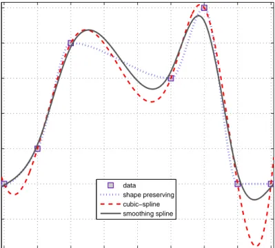
Three curve-fitting methods are considered in this work:
In shape-preserving interpolation, the fitted curve passes through the measure-ment points around which it is curvy and smooth but looks almost like straight lines in between. Hence, this method is very similar to linear (or first-order) interpolation except that the curve is differentiable everywhere. The fitted curve has high curvature, especially around the peaks.
The second method is cubic-spline interpolation. The curve in this method passes through the measurement points, like the previous one, but overall is much smoother. The fitted curve may oscillate unnecessarily in between the measurement points and may go far beyond the peaks of the measurements, in which case, it may not resemble (one axis of) the actual position curve of the tag. The smoothing spline is the third method, having a single parameter
ad-justable between 0 and 1. It is observed that this method resembles
shape-preserving interpolant when the parameter is chosen about 0.5 and cubic-spline interpolant when it is approximately 1. The parameter value should be chosen
proportionately large with the complexity of the data, i.e., the number of avail-able position measurements. In this study, we have used a parameter value of
1 − 10−6 for smoothing spline interpolation.
Although the third method seems to provide better results than the others, it is not feasible for long data as in this study since its computational complexity is much higher than the others. Therefore, we preferred to use shape-preserving interpolation because of its simplicity. Sample curves fitted to synthetic position data using the three methods are plotted in Figure 2.4. In addition, the x position of tag 4 in the fifth experiment of the fifth subject is plotted in Figure 2.5. Once the 12 different curves are fitted to the 12 axes of each experiment independently, the curves are re-sampled uniformly at exactly the same time instants.
1 2 3 4 5 6 7 8 9 0 1 2 3 4 5 6 time position
Simple example created to compare curve−fitting types (not to scale)
data
shape preserving cubic−spline smoothing spline
0 20 40 60 80 100 120 140 160 180 0 0.5 1 1.5 2 time (s) x (m)
position of tag 4 along x−axis in the experiment 5 of subject 5
data shape−preserving interpolation cubic−spline interpolation smoothing spline (a) 110 110.5 111 111.5 112 112.5 113 113.5 114 114.5 115 0.1 0.2 0.3 0.4 0.5 0.6 time (s) x (m) (b)
Figure 2.5: The x position of tag 4 in the fifth experiment of the fifth subject. (a) The whole curve and (b) the zoomed-in version.
2.2.2
Segmentation
After the curve fitting and uniform re-sampling stages, the modified dataset now consists of 5×5 = 25 2-D arrays (each corresponding to an experiment) with each line containing the time instant, position values along the 12 axes (three axes per tag) at that instant and the activity being performed at that time. Note that the number of rows is not the same in all of the experiments, since the duration of the experiment, hence the number of equally-spaced samples may differ slightly.
The 2-D array of each experiment is first divided into intervals containing samples corresponding to exactly one activity type. Then, each interval is divided into time segments of equal length, typically about one second. To prevent a segment from containing more than one activity, the following segmentation rule is used: For each experiment, progressing vertically along the 2-D array, a new segment is started only if the desired segment length is reached or a different activity is encountered. Naturally, the segments immediately before the transition points between activities and the very last segment may be shorter in length.
Classification is performed for each segment independently. While testing the classifiers and implementing the system in real time, the system needs to know where a new activity starts (i.e., the activity transition times). If this is not possible so that a constant segment duration is used, a segment may be associated with more than one activity. One can assign the longest activity contained in that segment as the true class, but this would unfairly decrease the classification accuracy. Since techniques for modeling activity durations and detecting the activity transition times are available [48, 52], we performed segmentation using the information on the true transition times so that each segment is associated with only a single activity.
2.3
Feature Extraction and Reduction
2.3.1
Feature Extraction
As stated above, each segment consists of many position samples in the corre-sponding time interval; each row of the dataset comprising 13 values (one time instant and 12 position values) as well as the true activity class. Thus, it would take a lot of time for a classifier to be trained and evaluated using the whole data. As an alternative, features extracted from the time segments are used for classification.
The features extracted for each of the 12 axes are the minimum, maxi-mum, mean, variance, skewness, kurtosis values, the first few coefficients of the autocorrelation sequence, and the magnitudes of the five largest FFT co-efficients. Therefore, there are (12 axes ×[11 + ceil(N/2)] coefficients per axis) = 132 + 12 × ceil(N/2) coefficients in the feature vector, N being the maximum number of samples in a segment (N = 5 in this study). Note that the size of the feature vector increases with the maximum number of samples in a segment which, in turn, is the product of the sampling frequency (in Hz) and the segment duration (in s).
2.3.2
Feature Reduction
Because of the large number of features (about 150–200) associated with each segment, we expect feature reduction to be very useful in this scheme. The size of the feature vector is reduced by mapping the original high-dimensional feature space to a lower-dimensional one using principal component analysis (PCA) and linear discriminant analysis (LDA) [53]. PCA is a transformation that finds the optimal linear combination of the features in the sense that they represent the data with the highest variance in a feature subspace, without taking the intra-class and inter-intra-class variances into consideration separately. It seeks a projection that best represents the data in a least-squares sense. On the other hand, LDA
seeks a projection that best separates the data in the same sense and maximizes class separability [53]. Whereas PCA seeks rotational transformations that are efficient for representation, LDA seeks those that are efficient for discrimination. The best projection in LDA makes the difference between the class means as large as possible relative to the variance.
2.4
Classification
The following are the 10 different classifiers used in this study, with their corre-sponding PRTools [54] functions:
(1) ldc: Gaussian classifier with the same arbitrary covariance matrix for each class
(2) qdc: Gaussian classifier with different arbitrary covariance matrices for each class
(3) udc: Gaussian classifier with different diagonal covariance matrices for each class
(4) mogc: mixture of Gaussians classifier (with two mixtures) (5) naivebc: na¨ıve Bayes classifier
(6) knnc: k-nearest neighbor (k-NN) classifier (7) kernelc: dissimilarity-based classifier
(8) fisherc: minimum least squares linear classifier (9) nmc: nearest mean classifier
(10) nmsc: scaled nearest mean classifier
2.5
Performance Evaluation through Cross
Val-idation
Since each of the five subjects repeats the same sequence of activities five times, the procedures used for training and testing affect the classification accuracy. For this reason, two different cross-validation techniques are used for evaluating the classifiers: P -fold and subject-based leave-one-out (L1O) [53].
In P -fold cross validation (P = 5 in this thesis), the whole set of feature vectors is divided into P partitions, where the feature vectors in each partition are selected completely randomly, regardless of the subject or the class they belong to. One of the P partitions is retained as the validation set for testing, and the remaining P − 1 partitions are used for training. The cross-validation process is then repeated P times (the folds), so that each of the P partitions is used exactly once for validation. The P results from the folds are then averaged to produce a single estimate of the overall classification accuracy.
In subject-based L1O cross validation, partitioning of the dataset is done subject-wise instead of randomly. The feature vectors of four of the subjects are used for training and the feature vectors of the remaining subject are used in turn for validation. This is repeated five times such that the feature vector set of each subject is used once as the validation data. The five correct classification rates are averaged to produce a single estimate. This is same as P -fold cross validation with P being equal to the number of subjects (P = 5) and all the feature vectors in the same partition being associated with the same subject.
Although these two cross-validation methods use all the data equally in train-ing and testtrain-ing of the classifiers, there are two factors that affect the results obtained based on the same data. The first one is the random partitioning of the data in the P -fold cross-validation technique that slightly affects the clas-sification accuracy. Secondly, classifier 7 (dissimilarity-based classifier) includes randomness in its nature. Therefore, both cross-validation methods are repeated five times and the average classification accuracy and its standard deviation are calculated over the five executions. This way, we can assess the repeatability of
the results and estimate how well the system will perform over newly acquired data from unfamiliar subjects.
2.6
Experimental Results
The following are the adjustable parameters or factors that possibly affect the classification accuracy, with their default values written in square brackets:
(1) fs: sampling frequency of the fitted curves in forming the modified data (in Hz) [default: 10 Hz]
(2) frm dur: maximum segment duration (in seconds) [default: 0.5 s] (3) curve fit type: the curve-fitting algorithm
(1: shape-preserving interpolation, 2: cubic-spline interpolation, 3: smoothing spline) [default: 1]
(4) pri: prior probabilities of the 11 classes (i.e., activities) (0: equal priors for each class,
1: priors calculated based on the class frequencies) [default: 1]
(5) reduc: the feature reduction type if used and the dimension of the reduced feature space
(0: no feature reduction; + |n|: PCA with reduced dimension n; − |n|: LDA with reduced dimension n) [default: 0]
All the classifiers are trained and tested using different combinations of the parameters described above. Then, for each classifier, the set of parameters that result in the lowest average classification error are determined. This process is repeated for both cases (the complete and the simplified classification problems with 11 and 5 classes, respectively) and both cross-validation methods (5-fold and subject-based L1O). Average classification errors of the classifiers over the five executions and their standard deviations are tabulated in Table 2.1. It is observed
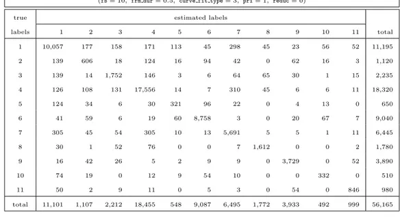
that the k-NN classifier (with k = 5) is the best one among the 10 classifiers compared in this study and outperforms the other classifiers in all cases. For the complete classification problem with 11 classes, the k-NN classifier has an average classification error of 8.67% and 21.30%, whereas for the reduced case with five classes, these numbers are 1.12% and 6.52% for 5-fold and subject-based L1O cross-validation, respectively. Note that since the partitions are fixed in subject-based L1O cross validation, this technique gives the same result if the complete cycle over the subject-based partitions is repeated. Therefore, its standard deviation is zero except for classifier 7 that includes randomness. For the k-NN classifier, the cumulative confusion matrices obtained by summing up the confusion matrices of each run in all of the five executions are presented in Tables 2.2 and 2.3 for the 11-class and 5-class problems, respectively, using the two cross-validation techniques.
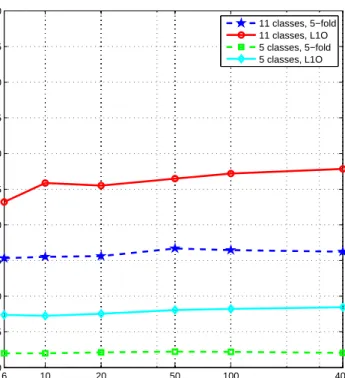
The parameters listed above significantly affect the classification accuracy. Therefore, for each parameter, the tests are run by varying that parameter while keeping the remaining ones constant at their default values. The variation of the average classification error with each of these parameters is shown in Fig-ures 2.6–2.10 for the two cross-validation methods and for both the complete and simplified classification problems (total of four cases). All the error percentage values presented in these figures are the average values over the five executions. Because the k-NN classifier (classifier 6) outperforms all of the other classifiers, the average classification error of only this classifier is shown in the figures. As expected, the 11-class classification problem results in larger errors compared to the 5-class problem. From the results, it can be observed that in all cases, 5-fold cross validation provides better results than subject-based L1O. This is because in the first case, the system is trained and tested with a random mixture of dif-ferent subjects’ data, whereas in the second, it is trained with the data of four of the subjects and tested with the data of the remaining subject which is totally new to the system.
classifier error p ercen tage ± standard deviation (with the corresp onding parameter v alues fs , frm dur , curve fit type , reduc ) 1 11 classes 5 classes 5-fold sub ject-based L1O 5-fold sub ject-based L1O 1 Gaussian classifier with the same arbitrary co v ariance matrix for eac h class 20.89 ± 0.02 23.52 6.06 ± 0.01 7.63 (10, 0.5, 1, –8) (10, 0.5, 3, – 8) (10, 0.5, 1, –4) (10, 0.5, 1, –4) 2 Gaussian classifier with differen t arbitrary co v ariance matrices for eac h class 20.76 ± 0.04 23.69 5.48 ± 0.02 7.73 (10, 0.5, 1, –6) (10, 0.5, 3, – 8) (10, 0.5, 1, –4) (10, 0.5, 1, –4) 3 Gaussian classifier with differen t diagonal co v ariance matrices for eac h class 21.65 ± 0.05 24.11 6.02 ± 0.02 7.92 (10, 0.5, 1, –6) (10, 0.5, 3, – 3) (10, 0.5, 1, –4) (10, 0.5, 1, –4) 4 mixture of Gaussians classifie r (with tw o mixtures) 20.75 ± 0.07 23.70 5.19 ± 0.03 7.63 (10, 0.5, 1, –6) (10, 0.5, 3, – 8) (10, 0.5, 1, –4) (10, 0.5, 1, –4) 5 na ¨ıv e Ba y es cl a ssi fier 22.84 ± 0.16 24.46 7.24 ± 0.16 9.49 (10–.5, 1, –8) (10, 0.5, 3, – 6) (10, 0.5, 1, –4) (10, 0.5, 1, –4) 8.67 ± 0.10 21.30 1.12 ± 0.04 6.52 6 k -NN classifier (k = 5) (10, 0.5, 3, 0) (10, 0.5, 1, – 10) (10, 0.2, 1, 0) (10, 0.2, 1, 0) 7 dissimilarit y-based classifier 19.41 ± 0.16 22.10 ± 0.04 4.66 ± 0.16 7.33 ± 0.03 (10, 0.5, 1, –8) (10, 0.5, 3, – 10) (10, 0.5, 1, –4) (10, 0.5, 1, –4) 8 minim um least squares linear classifier 25.26 ± 0.52 26.83 7.37 ± 0.17 9.30 (10, 0.5, 3, – 10) (10, 1, 3, 0) (10, 0.5, 1, –4) (10, 1, 1, 0) 9 nearest mean classifier 23.60 ± 0.06 27.02 6.07 ± 0.02 8.21 (10, 0.5, 3, – 10) (10, 0.5, 3, – 10) (10, 0.5, 1, –4) (10, 0.5, 1, –4) 10 scaled nearest mean classifier 20.94 ± 0.04 23.59 6.04 ± 0.03 7.58 (10, 0.5, 3, –8) (10, 0.5, 3, – 8) (10, 0.5, 1, –4) (10, 0.5, 1, –4) T able 2.1: The a v erage probabilit y of error (w eigh ted b y prior probabili ties) of the 10 classifiers, for the 11-and 5-class problems and the tw o cross-v al idation tec h niques. In eac h case, the com bination of param eters leading to the most accurate classifier is giv en in paran theses. pri = 1 throughout the table; that is, p rior probabiliti es are calculated from the class frequencies.
cumulative confusion matrix of classifier 6 (k-NN) for 5-fold (average classification error: 8.67%)
(fs = 10, frm dur = 0.5, curve fit type = 3, pri = 1, reduc = 0)
true estimated labels
labels 1 2 3 4 5 6 7 8 9 10 11 total 1 10,057 177 158 171 113 45 298 45 23 56 52 11,195 2 139 606 18 124 16 94 42 0 62 16 3 1,120 3 139 14 1,752 146 3 6 64 65 30 1 15 2,235 4 126 108 131 17,556 14 7 310 45 6 6 11 18,320 5 124 34 6 30 321 96 22 0 4 13 0 650 6 41 59 6 19 60 8,758 3 0 20 67 7 9,040 7 305 45 54 305 10 13 5,691 5 5 1 11 6,445 8 30 1 52 76 0 0 7 1,612 0 0 2 1,780 9 16 42 26 5 2 9 9 0 3,729 0 52 3,890 10 74 19 0 12 9 54 10 0 0 332 0 510 11 50 2 9 11 0 5 3 0 54 0 846 980 total 11,101 1,107 2,212 18,455 548 9,087 6,495 1,772 3,933 492 999 56,165
cumulative confusion matrix of classifier 6 (k-NN) for subject-based L1O (average classification error: 21.30%)
(fs = 10, frm dur = 0.5, curve fit type = 1, pri = 1, reduc = −10)
true estimated labels
labels 1 2 3 4 5 6 7 8 9 10 11 total 1 10,645 30 65 15 30 195 190 0 5 10 10 11,195 2 305 340 10 135 10 115 170 5 25 0 5 1,120 3 215 20 510 415 15 80 850 85 0 10 35 2,235 4 40 100 220 16,665 0 30 575 350 285 0 55 18,320 5 180 20 25 5 110 190 95 0 0 25 0 650 6 310 30 45 20 85 8,390 135 0 10 0 15 9,040 7 685 110 355 1,385 50 235 3,110 215 75 25 200 6,445 8 5 10 50 625 5 20 370 630 10 0 55 1,780 9 0 50 0 135 5 175 60 0 3,380 0 85 3,890 10 180 5 30 0 40 150 80 0 5 20 0 510 11 110 0 0 25 20 60 200 5 140 0 420 980 total 12,675 715 1,310 19,425 370 9,640 5,835 1,290 3,935 90 880 56,165
Table 2.2: Cumulative confusion matrices for classifier 6 (k-NN) for the 11-class problem. The confusion matrices are summed up for the five executions of the 5-fold (top) and subject-based L1O (bottom) cross validation.
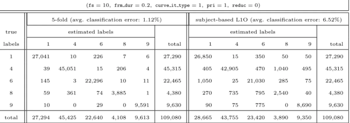
cumulative confusion matrices of classifier 6 (k-NN)
(fs = 10, frm dur = 0.2, curve it type = 1, pri = 1, reduc = 0)
5-fold (avg. classification error: 1.12%) subject-based L1O (avg. classification error: 6.52%)
true estimated labels estimated labels
labels 1 4 6 8 9 total 1 4 6 8 9 total
1 27,041 10 226 7 6 27,290 26,850 15 350 50 50 27,290 4 39 45,051 15 206 4 45,315 405 42,905 470 1,040 495 45,315 6 145 3 22,296 10 11 22,465 1,050 25 21,030 285 75 22,465 8 59 361 74 3,885 1 4,380 270 735 795 2,540 40 4,380 9 10 0 29 0 9,591 9,630 90 75 775 0 8,690 9,630 total 27,294 45,425 22,640 4,108 9,613 109,080 28,665 43,755 23,420 3,890 9,350 109,080
Table 2.3: Cumulative confusion matrices for classifier 6 (k-NN) for the 5-class problem. The confusion matrices are summed up for the five executions of the 5-fold (left) and subject-based L1O (right) cross validation.
2.6.1
Effect of the Sampling Frequency (fs)
When the sampling frequency is set too low, in particular, 6 Hz, the classification accuracy is surprisingly acceptable. This is because the movement of the RF tags is not very fast, and the classification performance does not degrade much when the high-frequency components are removed.
The average classification error increases slightly with increasing sampling rate (Figure 2.6). For instance, with fs = 400 Hz, noting that the dimension of the feature space also increases with the number of samples in a segment, the data becomes too complicated that it misleads most of the classifiers. This is because the position measurements are quite noisy; hence, selecting a high sampling rate may cause over fitting, which in turn degrades the classification accuracy of the system. A suitable value of fs is determined as 10 Hz and is set to be the default value. 6 10 20 50 100 400 0 5 10 15 20 25 30 35 40 45 50 sampling frequency (Hz)
average classification error (%)
11 classes, 5−fold 11 classes, L1O 5 classes, 5−fold 5 classes, L1O
Figure 2.6: Effect of the sampling frequency on the average classification error of the k-NN classifier (classifier 6).
2.6.2
Effect of the Segment Duration (frm dur)
Since a single event or activity is associated with each segment, the segment duration is another parameter that affects the accuracy. Results for segment duration values between 0.2 s and 1 s are shown in Figure 2.7. Although the smallest segment duration gives slightly better results in most cases, the system should make a decision five times in a second with this segment duration, which increases the complexity. In fact, even a very short segment consisting of a single position measurement (one row of the dataset) is sufficient to obtain the body posture information since it directly provides the 3-D positions of the tags on
different body parts at that instant. Compromising between complexity and
accuracy, a segment duration of 0.5 s is selected as the default value without much loss in the classification accuracy in each of the four cases.
0.2 0.3 0.4 0.5 0.7 1 0 5 10 15 20 25 30 35 40 45 50 segment duration (s)
average classification error (%)
11 classes, 5−fold 11 classes, L1O 5 classes, 5−fold 5 classes, L1O
Figure 2.7: Effect of the the segment duration on the average classification error of the k-NN classifier (classifier 6).
2.6.3
Effect of the Curve-Fitting Algorithm
Referring to Figure 2.8, it is observed that shape-preserving interpolation and cubic-spline interpolation give very similar results for subject-based L1O whereas the smoothing spline interpolation leads to poorer classification accuracy. The lat-ter is the best curve-fitting method in the particular case of 5-fold cross-validation with 11 classes. Thus, shape-preserving interpolation is chosen as the default curve-fitting method.
shape−preserving cubic−spline smoothing spline 0 5 10 15 20 25 30 35 40 45 50
curve fitting method
average classification error (%)
11 classes, 5−fold 11 classes, L1O 5 classes, 5−fold 5 classes, L1O
Figure 2.8: Effect of the curve-fitting method on the average classification error of the k-NN classifier (classifier 6).
2.6.4
Effect of the Prior Probabilities
Classification errors for the individual classes can be obtained from the confusion matrices provided in Tables 2.2 and 2.3. The average probability of error is calcu-lated by weighting the classification error of each class with its prior probability. In this study, prior class probabilities have been chosen in two different ways. In the first, prior probabilities are taken equal for each class, whereas in the second, prior probabilities are set equal to the actual occurrence of the classes in the data. Figure 2.9 illustrates the effect of prior probabilities on the average classification error. It is observed in the figure that the error for the case with equal priors is larger. This is because the transition classes (Section 2.2.2) rarely occur in the dataset and their probability of occurrence is extremely low. However, the classification errors for these classes are larger. When a weighted average is cal-culated using the actual class probabilities, those terms with large classification error contribute relatively less to the total average error.
equal priors priors from class freq. 0 5 10 15 20 25 30 35 40 45 50 prior probabilities
average classification error (%)
11 classes, 5−fold 11 classes, L1O 5 classes, 5−fold 5 classes, L1O
Figure 2.9: Effect of the prior probabilities on the average classification error of the k-NN classifier (classifier 6).
2.6.5
Effect of Feature Reduction
Since there is a large number of features (depending on the sampling frequency and the segment duration), two common methods (PCA and LDA) are used for feature reduction. All the results up to this point, including Figures 2.6–2.9, are obtained without feature reduction.
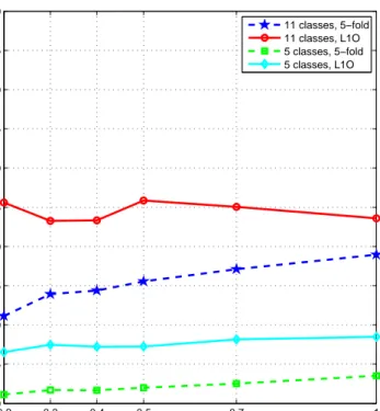
Figure 2.10(a) shows the average classification error when PCA is used with different reduced dimensionalities (from 1 to 100) as well as the case without feature reduction (168). It can be observed that the intrinsic dimensionality of the feature vectors is about 10, which is much smaller than the actual dimension. Figure 2.10(b) corresponds to the cases where LDA is used with reduced di-mension from 1 to 10 for 11 classes and from 1 to 4 for 5 classes (note that reduced dimension must be less than the number of classes in LDA). For the complete classification problem with 11 classes, LDA with dimension 10 outperforms all other cases including the ones without feature reduction validated by subject-based L1O. Including too many features not only increases the computational complexity of the system significantly, but also confuses the classifiers, leading to a less accurate system (this is known as “the curse of dimensionality”).
For the 11-class problem, LDA with dimension 10 performs better than PCA when L1O is used and worse when 5-fold cross validation is employed. For the simplified problem with 5 classes, the results change similarly with feature reduc-tion. With subject-based L1O, LDA with dimension four outperforms PCA with higher dimensions as well as the case without feature reduction. When 5-fold cross-validation is used, PCA with dimension 20 is the best one. Hence, LDA with dimension four is preferable because its performance seems to be less depen-dent on the subject performing the activities. Therefore, it can be stated that LDA is more reliable if the system is going to be used with subjects who are not involved in the training process. On the other hand, if the system is going to be trained for each subject separately, PCA results in a more accurate classifier, even at the same dimensionality with LDA.
1235710 20 30 40 50 70 100 168* 0 5 10 15 20 25 30 35 40 45 50
dimension of the reduced space (*: without feature reduction)
average classification error (%)
11 classes, 5−fold 11 classes, L1O 5 classes, 5−fold 5 classes, L1O (a) 1 2 3 4 6 8 10 0 5 10 15 20 25 30 35 40 45 50
dimension of the reduced space
average classification error (%)
11 classes, 5−fold 11 classes, L1O 5 classes, 5−fold 5 classes, L1O
(b)
Figure 2.10: Effect of feature reduction with (a) PCA and (b) LDA on the average classification error of the k-NN classifier (classifier 6).
2.7
Conclusion
In this study, a novel approach to human activity recognition is presented using a tag-based RF localization system. Accurate activity recognition is achieved without the need to consider the interaction of the subject with the objects in its environment. In this scheme, the subjects wear four RF tags whose positions are measured via multiple antennas (readers) fixed to the environment.
The most important issue is the asynchronous and non-uniform acquisition of the position data since the system records measurements whenever it detects a tag, and the detection frequency is affected by the SNR and interference in the environment. The asynchronous nature of the data acquired introduces some additional problems to be tackled—only one tag can be detected at a given time instant; hence, the measurements of different tags are acquired at different time instants in a random manner. This problem has been solved by first fitting a suitable curve to each measurement axis along time, and then re-sampling the fitted curves uniformly at a higher sampling rate at exactly the same time instants. After the uniformly-sampled curves are obtained, they are partitioned into segments of maximum duration of one second each such that each segment is associated with only a single activity type. Then, various features are extracted from the segments to be used in the classification process. The number of features are reduced using two feature reduction techniques.
Ten different classifiers are investigated and their average classification er-rors are calculated for various curve-fitting and feature reduction techniques and system parameters. In calculating the average classification error, two different cross-validation techniques, namely P -fold with P = 5 and subject-based L1O, are used. Omitting the transition classes, the complete pattern recognition prob-lem with 11 classes is reduced to a probprob-lem with five classes and the whole process is repeated. Finally, the set of parameters and the classifier giving the best result is presented for each problem and for each cross-validation method.
For the complete problem with 11 classes, the proposed system has an aver-age classification error of 8.67% and 21.30% when the 5-fold and subject-based

![Figure 2.1: Ubisense hardware components [14].](https://thumb-eu.123doks.com/thumbv2/9libnet/5987232.125641/27.892.303.660.172.466/figure-ubisense-hardware-components.webp)