NUMERICAL AND EXPERIMENTAL
INVESTIGATION OF THE EFFECT OF
CHANNEL GEOMETRY ON CAVITY
FORMATION IN MICROFLUIDIC
CHANNELS
a thesis submitted to
the graduate school of engineering and science
of bilkent university
in partial fulfillment of the requirements for
the degree of
master of science
in
mechanical engineering
By
G¨
ok¸ce ¨
Ozkazan¸c
June 2020
NUMERICAL AND EXPERIMENTAL INVESTIGATION OF THE EFFECT OF CHANNEL GEOMETRY ON CAVITY FORMATION IN MICROFLUIDIC CHANNELS
By G¨ok¸ce ¨Ozkazan¸c June 2020
We certify that we have read this thesis and that in our opinion it is fully adequate, in scope and in quality, as a thesis for the degree of Master of Science.
E. Yegan Erdem(Advisor)
Levent ¨Unl¨usoy(Co-Advisor)
Barbaros C¸ etin
Ali Ko¸sar
Approved for the Graduate School of Engineering and Science:
ABSTRACT
NUMERICAL AND EXPERIMENTAL
INVESTIGATION OF THE EFFECT OF CHANNEL
GEOMETRY ON CAVITY FORMATION IN
MICROFLUIDIC CHANNELS
G¨ok¸ce ¨Ozkazan¸c
M.S. in Mechanical Engineering Advisor: E. Yegan Erdem Co-Advisor: Levent ¨Unl¨usoy
June 2020
Cavitation formation in low pressure regions of a flow is a chaotic distortion in fluid mechanics. Due to the complicated nature of multiphase flows, its modelling is expensive in terms of time and computational power. Opensource softwares such as OpenFOAM reduce license expenses and provide a developer friendly environment to simulate these types of complicated flows. In this thesis, by using OpenFoam software, several different geometries that cause cavitation are investigated. Presented results are compared with both literature and supported by experimental results. Experiments are carried out in microfluidic chips that are fabricated with soft lithography technique; fluorescent particles were introduced in the flow and cavity formation was observed under a fluorescent camera. Results showed that, OpenFOAM is well capable of predicting the cavitation formation in small scales. It was observed that increasing channel width reduces the pressure difference causing bubbles to form in higher input pressures. It was also seen that decreasing the channel width causes friction and viscous forces to dominate and reduce the velocity of fluid preventing the cavitation to form. Overall the modelling of cavity formation in microchannels with varying width and cross sectional profile were successfully accomplished and results were verified with experiments.
¨
OZET
M˙IKRO KANALLARDA KANAL GEOMETR˙IS˙IN˙IN
KAV˙ITASYON OLUS
¸UMU ¨
UZER˙INDEK˙I ETK˙IS˙IN˙IN
SAYISAL VE DENEYSEL OLARAK ˙INCELENMES˙I
G¨ok¸ce ¨Ozkazan¸c
Makine M¨uhendisli˘gi, Y¨uksek Lisans Tez Danı¸smanı: E. Yegan Erdem ˙Ikinci Tez Danı¸smanı: Levent ¨Unl¨usoy
Haziran 2020
D¨u¸s¨uk basın¸clı b¨olgelerdeki kavitasyon olu¸sumu, akı¸skanlar mekani˘ginde kaotic bir bozulmaya sebep olmaktadır. Karma¸sık do˘gası sebebiyle bu tarz ¸cok fazlı akı¸s modellemeleri hem zaman hem de bilgisayar g¨uc¨u olarak pahalı olmak-tadır. Bu modelleme ¸calı¸smalarının OpenFOAM gibi a¸cık kaynaklı yazılımlar ile yapılması ise hem lisans maliyetni d¨u¸s¨urmekte hem de, i¸cerisinde kolayca de˘gi¸siklilk yapılmasına izin vermektedir. Bu kapsamda yapılan tez ¸calı¸smasında, OpenFOAM yazılımı kullanılarak, kavitasyon olu¸sabilecek farklı geometriler in-celenmi¸stir. Elde edilen sonu¸clar hem literat¨ur hem de yapılan deneyler ile kar¸sıla¸stırılmı¸stır. C¸ ipler yumu¸sak fotolitografi ile ¨uretilmi¸s ve florans par¸cacıklar ile karı¸stılan akı¸s florans mikraskobu ile g¨or¨unt¨ulenmi¸stir. Sonu¸clar Open-FOAM’un bu tip bir modellemeyi yapabildi˘gini g¨ostermi¸stir. Kanal ¸capının arttırılmasının, baloncuk olu¸sumunu sa˘glayan basın¸c d¨u¸s¨u¸s¨un¨u azaltmaktadır. Aynı zamanda kanal ¸capının d¨u¸s¨ur¨ulmesinin ise s¨urt¨unme ve viskoz kuvvet-lerin baskın hale gelmesine sebep oldu˘gu g¨or¨ulm¨u¸st¨ur. Sonu¸c olarak, mikro kanallarda farklı geometrilerde incelenen kavitasyon olu¸sumu ba¸sarılı bir ¸sekilde g¨ozlemlenmi¸s ve deneyler ile do˘grulanmı¸stır.
inter-Acknowledgement
From the start of my undergraduate education till the end of this project and even after that, I am thankful to my family for making this possible. I would not be able to succeed without their patience, support and presence.
Also, I would like to thank my advisor Asst. Prof. Yegan Erdem for her unconditional support and guidance. Her patience and vision gave me the energy and motivation to continue. Without her, nothing would be as it is now. I would also like to thank Dr. Barbaros C¸ etin and Dr. Ali Ko¸sar for their critics and time as the thesis committee.
As a mentor and advisor, I am thanking to my co-advisor Dr. Levent ¨Unl¨usoy for guiding me through this project. It was an honour to work with him.
I would also like to thank O.Berkay Sahinoglu for being the most enjoyable lab partner and making the experiments easier and more fun.
As a friend, partner in crime and a family to me, I am especially grateful for Furkan G¨u¸c’s presence, he gave me the energy and strength to keep on even when I did not know that I needed.
Lastly, I would like to acknowledge the Presidency of Defence Industries, SSB, for financially supporting this research under SAYP Program.
Contents
1 Introduction 8
1.1 Thesis Overview . . . 10
2 Measurements, Equations and Numerical Methods and Algo-rithms 11 2.1 Boundary Conditions . . . 11
2.2 Coupling Experiments with Simulation . . . 12
2.3 Governing Equations . . . 14
2.3.1 Presure-Velocity Calculations . . . 16
2.4 OpenFOAM Structure . . . 17
2.4.1 Solvers . . . 18
3 Development of Analysis Methodology 20 3.1 Verification of Boundary Conditions . . . 21
CONTENTS vii
3.1.2 simpleFOAM . . . 23
3.1.3 pimpleFoam . . . 25
3.1.4 interPhaseChangeFoam . . . 25
3.2 Geometries . . . 31
3.2.1 Single Channel Throttle Model and Configurations . . . . 31
3.2.2 Double Channel Geometry . . . 35
3.2.3 Triple Channel Geometry . . . 36
3.2.4 Nozzle Inspired Channel Geometry . . . 37
3.2.5 Double Inclined Geometry . . . 39
4 Calculations and Simulation Results 41 4.1 Single Channel Throttle Geometry . . . 42
4.1.1 Coefficient Calculations . . . 42
4.1.2 Effect of Input Pressure . . . 53
4.1.3 Effect of Channel Thickness . . . 55
4.2 Double Channel Geometry . . . 57
4.3 Triple Channel Geometry . . . 59
4.4 Nozzle Inspired Channel Geometry . . . 62
CONTENTS viii
5 Experimental Set-up, Fabrication and Results 67
5.1 Set-Up . . . 67
5.2 Fabrication of Microfluidic Chips . . . 69
5.3 Experimental Results . . . 74
6 Conclusion and Future Work 80 A Code 88 B Results 92 B.0.1 Discharge Coefficient Results . . . 92
B.0.2 Effect of Input Pressure Results . . . 94
B.0.3 DhRe/L vs. Reynolds Number Table . . . 95
B.0.4 CFD Results . . . 96
C Masks 102
List of Tables
2.1 Stable Boundary Conditions . . . 12
2.2 Properties of Labelled Sections . . . 13
2.3 Measured Properties in the Set-up . . . 15
3.1 Calculated Reynolds Number . . . 22
3.2 Boundary Conditions Implemented in OpenFoam . . . 24
3.3 Maximum Velocity Values Obtained in OpenFoam Solvers and An-alytical Solution . . . 26
3.4 Configurations of Single Throttle Geometry . . . 32
3.5 Total cells of the meshes . . . 32
3.6 Total cells of the meshes . . . 35
3.7 Dimensions of the Geometry . . . 37
3.8 Dimensions of the Geometry . . . 39
LIST OF TABLES x
4.2 Contraction Coefficient Results for single throttle geometry . . . . 47
4.3 Percentage Errors for Discharge Coefficient in Single Channel Ge-ometry . . . 51
5.1 Spin parameters for base layer . . . 69
5.2 Spin parameters for main layer . . . 70
List of Figures
2.1 Representation of the flow in the experimental set-up . . . 13
2.2 Measured Flow Rate Values in Different Input Pressures . . . 14
2.3 Solution Algorithm’s of a) SIMPLE and b) PISO . . . 17
2.4 Solution Algorithm of PIMPLE . . . 18
2.5 Case File of Simulations . . . 19
3.1 Step by Step Methodology of Model Development . . . 20
3.2 Rectangular channel and its dimensions for analytical solution . . 22
3.3 Velocity contour obtained from analytical solution with MATLAB 23 3.4 Rectangular channel and its dimensions for analytical solution . . 23
3.5 Mesh generated for SimpleFoam . . . 24
3.6 Solution of SimpleFoam . . . 24
3.7 Solution of pimpleFoam . . . 25
3.9 Velocity profile of the channel (a) with a detailed view (b) . . . . 27 3.10 Velocity profile of the channel (a) with a detailed view (b) . . . . 28 3.11 Velocity difference 2D and 3D simulations . . . 29 3.12 Pressure difference in 2D and 3D simulations . . . 30 3.13 Geometry and boundary conditions of throttle configuration . . . 31 3.14 a) Coarse, b) Middle and c) Fine meshe sizes created for single
throttle configuration . . . 33 3.15 Axial velocity profiles for coarse, middle and fine meshes in the
throttle . . . 34 3.16 Clock time change according to the number of CPU’s . . . 34 3.17 Geometry and boundary conditions of double throttle channel
ge-ometry . . . 35 3.18 Grid of the double throttle channel geometry . . . 36 3.19 Geometry and boundary conditions of triple channel geometry . . 36 3.20 Grid of the triple channel geometry . . . 37 3.21 Geometry and boundary conditions of nozzle inspired channel
ge-ometry . . . 38 3.22 Grid of the nozzle type channel geometry . . . 38 3.23 Geometry and boundary conditions double inclined channel
geom-etry . . . 39 3.24 Grid of the double inclined channel geometry . . . 40
4.1 Representation of Vena Contracta . . . 42
4.2 Location of vena contracta for different channel types) a) β = 0, 12 and A=0,6, b) β = 0, 16 and A=0,8 and c) β = 0, 20 and A=1,0 . 43 4.3 Location of vena contracta for different channel types) a) β = 0, 12 and A=0,6, b) β = 0, 12 and A=0,5 and c) β = 0, 12 and A=0,4 d) β = 0, 12 and A=0,3 . . . 44
4.4 Location of vena contracta for different Reynolds numbers a) Re=25 b) Re=42.6 and c) Re=58 . . . 45
4.5 Contraction Coefficient with respect to the Square Root of Reynolds number . . . 46
4.6 Discharge Coefficient with respect to the Square Root of Reynolds number . . . 49
4.7 Discharge Coefficient of β=0,06 and A=0,3 . . . 50
4.8 Discharge Coefficient of β=0,16 ans A=0,8 . . . 50
4.9 Discharge Coefficient of β=0,24 and A=1,2 . . . 51
4.10 Percentage Error in Discharge Coefficient calculations . . . 52
4.11 Velocity coefficient results for single channel Geometry . . . 53
4.12 Pressure change along the channel at t=0.00013s for different inlet pressures . . . 54
4.13 Phase change at different input pressures . . . 55
4.14 Representation of the Flow in the Experimental Set-up . . . 56
4.16 Velocity Contour with Respect to Time for Double Channel Ge-ometry . . . 57 4.17 Pressure Change in Channels in Double Channel Geometry . . . 58 4.18 Alpha Contour with Respect to Time For Double Channel Geometry 59 4.19 Velocity Contour with Respect to Time for Triple Channel
Geom-etry . . . 60 4.20 Pressure Change in Channels in Triple CHannel Geometry . . . . 61 4.21 Alpha Contour with Respect to Time for Triple channel geometry 61 4.22 Velocity contour with respect to time for nozzle type channel
ge-ometry . . . 62 4.23 Velocity contour with respect to time for nozzle type channel
ge-ometry . . . 63 4.24 Pressure changes along the centerline of the nozzle inspired
geome-tries . . . 64 4.25 Angles in between channels . . . 65 4.26 Velocity contour with respect to time for nozzle type channel
ge-ometry . . . 66 4.27 Alpha contour with respect to time for nozzle type channel
geom-etry . . . 66
5.1 Experimental Set up . . . 68 5.2 Photolithography technique to produce microchips with negative
5.3 Visuals of the producted chips . . . 73
5.4 Steady flow in 30 micron width channel with 3 bars input pressure 74 5.5 Steady flow in nozzle inspired geometry with 3 bars input pressure 74 5.6 Vapour Bubble in the 30 Micron Channel . . . 75
5.7 Simulation vs. Experimental Low Density Zones . . . 75
5.8 Symmetrical Low Density Zones in Simulation and Experiments . 76 5.9 Vortex region (a) and its movement (b) . . . 77
5.10 Cavitation Zone . . . 78
5.11 Symmetrical Low Density Zones . . . 78
5.12 Cavitation Bubble with Degasified Water . . . 79
B.1 β=0,1 and A=0,5 . . . 92
B.2 β=0,12 ans A=0,6 . . . 93
B.3 β=0,20 and A=1,0 . . . 93
B.4 Velocity Along the channel centerline in different pressure inputs . 94 B.5 Pressure contour with respect to time for double channel geometry 96 B.6 Pressure contour with respect to time for triple channel geometry 97 B.7 Pressure contour with respect to time for nozzle inspired channel geometry . . . 98 B.8 Pressure contour with respect to time for nozzle inspired channel
B.9 Pressure contour with respect to time for nozzle inspired channel geometry . . . 99 B.10 Pressure contour with respect to time for nozzle inspired channel
geometry . . . 99 B.11 Pressure contour with respect to time for double inclined geometry 100 B.12 Velocity vectors with respect to time for double inclined geometry 101
C.1 Mask 1 . . . 102 C.2 Mask 2 . . . 103
Nomenclature
µ Viscosity ρ Density g Gravitational Acceleration H Channel Thickness h Channel width h HeightL Length of the entrance section Pst Static Pressure
Ptot Total pressure
Q Flow Rate
W Width of the entrance section u X Velocity
v Y Velocity w Z Velocity
Chapter 1
Introduction
One of the commonly used techniques to cool down a high temperature com-bustion chamber is by circulating a coolant fluid around its shell in a small channel [1, 2]. However, as the pressure drops along the channel, fluid inside the channel changes its phase and decreases the efficiency of the cooling proce-dure [3], which is known as cavitation. In other words cavitation, can be defined in detail as the phase change of the fluid flow by nucleation, growth and collapse of a vapour bubble in regions where pressure drop is rapid and high [4].
The damaging effects of cavitation are undesired not only in cooling channels but also in most of the applications that includes high speed fluid flows such as nozzles [5], hydraulic machinery [6] and diesel engines [7]. Therefore, before going further in the design process of these applications, predicting these unwanted phase changes is playing an important role to reduce both the time and expenses of the system.
To predict such behaviour, several different numerical and modeling methods have already been developed [8] such as the empirical study of Shi et al. [9] or the steady state approach of Hanimann et al. [10] or on the contrary using a highly transient model as Large Eddy Simulation (LES) approaches [11, 12].
One common point in all of these different approaches is that the modelling of cavitation is expensive in terms of both computational power and time. To minimize this cost, the usage of open source softwares are emerging [13, 14]. OpenFOAM, as an opensource tool is one of the most preferred tools due to its C++ language and adaptability by the users [15] for this purpose.
On top of that, with the development of microrockets and micropropulsion systems, micropumps, microturbomachinery, etc. that creates high speed flows in microchannels, cavitation studies also merged with microfluidic applications [16]. Even though there are studies that investigated the cavitation behaviour in various types of geometries [17, 18] throttle (orifice) and venturi geometries are the main interest in the studies of cavitation in microchannels [19–21]. Therefore a variety of studies such as testing the cavitation properties of different fluids [22], predicting the possible locations of cavitation [23], effect of surface roughness [24] and experiments [19, 20, 24–28] are also focused around this geometry.
The motivation of this study consists of developing the methodology of cavita-tion modeling in a cost efficient manner. It is expensive to conduct experiments on large scaled systems about cavitation in industrial applications. Therefore those systems require low cost verification and validation procedures of the com-putational fluid dynamics solvers. This study aims to verify and validate the OpenFOAM solver of interPhaseChangeFOAM in small scaled channels with re-ducing the experiment cost by using microchannels. With this way, its usability in industrial applications such as predicting the cavitation behaviour in cooling channels of combustion chambers, will also be shown with a quick and low cost approach. Therefore, the solvers mainly aim to show the applicability of the pro-posed method in macro-systems in an efficient way by using a low experimental and computational cost.
1.1
Thesis Overview
In this study, cavitation will be investigated from many aspects. Firstly, apart from the common geometries, behaviour of flow in different type of channels will be presented. Also, capability of OpenFOAM in small scales will be observed with the comparison of literature and experiments. With this concept, the overview of the thesis can be summarized as follows:
• Chapter 2 describes the measurements to couple the experiments with the simulations that are held on OpenFOAM as well as it introduces the main governing equations.
• Chapter 3 mainly describes the structure of OpenFoam and the solvers that it includes.
• Chapter 4 explains the choice of boundary conditions with a validation case and presents its results, leading to the simulation strategy. Geometries of the simulations are also explained in detail in this chapter.
• Chapter 5 includes the calculations of coefficients to validate the simulations and its comparison with literature. Also, results of the simulations are presented here.
• Chapter 6 explains the experimental set up that is built to conduct exper-iments.
• Chapter 7 presents the visuals obtained from the experiments and compar-ison to the simulations conducted.
• Chapter 8 is the conclusion that sums up the work conducted throughout this study and suggests future work to improve the performance of both experiments and simulations.
Chapter 2
Measurements, Equations and
Numerical Methods and
Algorithms
In this section, governing equations will be discussed. First section describes the exact equations and results that are used in simulations and second part describes the main equations and algorithms used by OpenFOAM foam-extend-4.1 with the description of main pressure-veloicty coupling algorithms.
2.1
Boundary Conditions
Several different boundary condition couples are available for pressure-velocity systems in OpenFOAM. These combinations are already tested and grouped together regarding their stability. For incompressible systems, these boundary condition couples are classified as given in Table 2.1 [29].
Table 2.1: Stable Boundary Conditions
Inlet Outlet Stability
Physics OpenFOAM Physics OpenFOAM
Volume Flow Rate flowRateVelocity Static Pressure fixedValue Excellent Total Pressure totalPressure Total Pressure totalPressure Very Good Total Pressure totalPressure Static Pressure fixedValue Good Static Pressure fixedValue Static Pressure fixedValue Poor Regarding the table, total pressure for an incompressible fluid is defined as [29];
Ptot = Pst+
1 2ρu
2
(2.1.1)
where Pst is the static pressure and the summation of pressure in the regarding
point and ρgh, u is the magnitude of the velocity vector and ρ is the density. As it is given in the equation, static pressure is known and the only unknown is the velocity, To be able to simulate the real life experimental values, velocity at the inlet must be learned. With this aim, next section explains the procedure for measuring the velocity at the inlet so that it could be implemented in the given equation 2.1 and used as a boundary condition value.
2.2
Coupling Experiments with Simulation
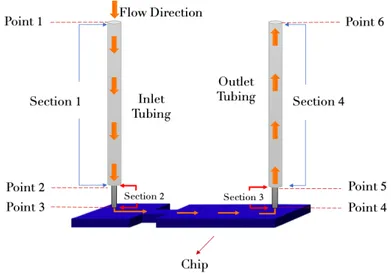
As an initial step for coupling simulations with experiments, velocity and pressure values of the critical points of the experimental set-up is calculated. To calculate these, experimental set-up is divided into several sections. These sections of control volume and geometrical representation of the flow path in the experiment is given in Figure 2.1. Points and sections, important for the calculations are also explicitly shown.
Figure 2.1: Representation of the flow in the experimental set-up Table 2.2: Properties of Labelled Sections
Section Area (m2) Length (m)
Section 1 2.0428e-07 0.31 Section 2 5.3093e-08 0.0166 Section 3 5.3093e-08 0.0166 Section 4 2.0428e-07 0.30
Flow rate entering the chip provided by the pressure pump is experimentally measured for several different pressure inputs. Values above the limit of the flow rate sensor (above 1ml/min [30]) were extrapolated through an exponential equation. Relevant graph of flow rate with respect to input pressure is given in Graph 2.2 below.
As a final step using hydraulic circuit analogy, pressure of the inlet section is calculated. All of the results are given in Table 2.3.
However, while modelling the simulations some phenomena are neglected since only the fluid flow inside the channels is simulated. These include surface rough-ness, hydrophobic and hydrophilic behaviour of the surfaces [31, 32]. These were neglected in order to satisfy the ease of use, implementation and repeatability of the analysis framework while capturing the requirements mentioned before.
Figure 2.2: Measured Flow Rate Values in Different Input Pressures
2.3
Governing Equations
For a compressible fluid, conservation of mass is written as;
∂ρ ∂t + ∂(ρu) ∂x + ∂(ρv) ∂y + ∂(ρw) ∂z = 0 (2.3.2)
where u, v and w are the relevant velocity vectors for the cartesian coordinates x,y and z. When fluid is incompressible, which corresponds to a constant density, equation 2.3.2 becomes as follows;
∂(ρu) ∂x + ∂(ρv) ∂y + ∂(ρw) ∂z = 0 (2.3.3)
Table 2.3: Measured Properties in the Set-up
Input Pressure Flow Rate Velocity Pressure at Total Pressure at Point 1 (P a) (m3/s) (m/s) Point 3 (P a) (P a) 10000 2.929e-09 0.05517 9037.294 100079.917 20000 5.341e-09 0.1006 18244.517 109290.677 30000 7.447e-09 0.1403 27552.316 118603.244 40000 9.101e-09 0.1714 37008.678 128064.467 50000 1.046e-08 0.1971 46562.002 137622.506 75000 1.409e-08 0.2655 70368.891 161445.236 85000 1.543e-08 0.2906 79928.459 171011.784 90000 1.612e-08 0.3035 84701.670 175788.826 100000 1.779e-08 0.3351 94152.773 185250.019 150000 2.424e-08 0.4565 142032.784 233178.080 200000 3.018e-08 0.5684 190080.422 281283.118 250000 3.578e-08 0.6739 238239.811 329507.981 300000 4.112e-08 0.7744 286484.656 377825.604 350000 4.624e-08 0.8710 334801.812 426222.233 400000 5.120e-08 0.9643 383171.557 474677.594 450000 5.601e-08 1.0549 431590.603 523188.216 500000 6.069e-08 1.1432 480052.378 571746.932 550000 6.527e-08 1.2293 528547.022 620343.711 600000 6.975e-08 1.3137 577074.533 668978.537 Regarding conservation of momentum equations for a compressible fluid in x, y and z coordinates are;
∂(ρu) ∂t + ∂(ρu2) ∂x + ∂(ρuv) ∂y + ∂(ρuw) ∂z = − ∂p ∂x + µ( ∂2u ∂x2 + ∂2u ∂y2 + ∂2u ∂z2) (2.3.4) ∂(ρv) ∂t + ∂(ρuv) ∂x + ∂(ρv2) ∂y + ∂(ρvw) ∂z = − ∂p ∂y + µ( ∂2v ∂x2 + ∂2v ∂y2 + ∂2v ∂z2) (2.3.5) ∂(ρw) ∂t + ∂(ρuw) ∂x + ∂(ρvw) ∂y + ∂(ρw2) ∂z = − ∂p ∂z + µ( ∂2w ∂x2 + ∂2w ∂y2 + ∂2w ∂z2 ) (2.3.6)
trans-∂(|u|)
∂t + 5(|u||u|) = − 1
ρ 5 + 5 (µ 5 |u|) (2.3.7)
2.3.1
Presure-Velocity Calculations
OpenFOAM uses three different algorithms for combining mass conservation, pressure and momentum equations [33]. These are, semi-implicit method for pressure-linked equations (SIMPLE) pressure-implicit split-operator (PISO) and PIMPLE algorithm which is combination of both SIMPLE and PISO algo-rithms [33]. Main difference of these three algoalgo-rithms can be summarized as follows; SIMPLE is used for modeling steady-state problems, PISO is used for transient problems with Courant Number limitation and PIMPLE is used for transient problems which requires bigger Courant Number (>1) [34]. Where Courant number is defined as follows;
Co = U 4 t
4x (2.3.1.8)
In this manner SIMPLE, PIMPLE and PISO algorithms are summarized in 2.3 and 2.4 [35].
(a) SIMPLE Algorithm (b) PISO Algorithm
Figure 2.3: Solution Algorithm’s of a) SIMPLE and b) PISO
2.4
OpenFOAM Structure
A basic OpenFOAM simulation requires 3 main subfolders which are ”0”, ”con-stant” and ”system”. Respectively, ”0” folder contains all the required boundary conditions for physical fields, ”constant” directory contains mesh information of the geometry, transport properties of the fluid/fluids and turbulence properties. Finally ”system” folder consists of solution based files such as numerical methods and simulation properties [15]. Each case runs with its relevant solver indicated in the system folder. Fields inside these folders may show diversity regarding the solver and the application, for this study all of the files are as the one given in Figure 2.5 below.
Figure 2.4: Solution Algorithm of PIMPLE
2.4.1
Solvers
OpenFOAM has many solvers adapted for modeling different physical phenom-ena. The ones that are used and discussed in this work are simpleFoam, pimple-Foam and interPhaseChangepimple-Foam.
SimpleFoam solver is defined as a steady solver for incompressible fluids, whereas pimpleFoam is the transient solver for incompressible fluids and finally interPhaseChangeFoam is the transient solver for two immiscible and incompress-ible fluids with changing phase [33].
Figure 2.5: Case File of Simulations
InterPhaseChangeFoam solver is the multiphase solver that uses volume of fluid method to model cavitation and it is the main solver used for this study. Its algorithm is based on PISO which is described previously [33]. The solver also uses the Volume of Fluid (VOF) method to capture the interface between phase change sections of the domain. with this solver several different cavitation models can be used such as The Merkle, Schnerr-Sauer and Kunz models. Mainly these models differ from each by the methods they capture the interphase between the volumes and the coefficients used by the volume fractions [36, 37]. In which, The Schnerr & Sauer Model that calculates the mixed bubble-liquid flow transiently is used for this study [37, 38].
Chapter 3
Development of Analysis
Methodology
Developing the analysis methodology for modelling cavitation in microchannels with OpenFOAM required several steps. With this aim, initially a simple ver-ification case solved was a channel flow. Steps taken in order to determine the methodology was summarized in Figure 3.1. Then section continues with the description of geometries that will be used for modelling cavitation in this study.
3.1
Verification of Boundary Conditions
This section explains the verification study for a pressure driven flow in a rect-angular channel solved with Matlab and its comparison to several solvers such as simpleFoam, pimpleFoam and interPhaseChangeFoam.
3.1.1
Analytical Solution
Studies were initially conducted on laminar channel flows which corresponds to Reynolds Number less than 2300 for most applications and calculated from the given equation below for the inlet region of the channel.
Re = V Lρ
µ (3.1.1.1)
in which, L is the length scale, V is the velocity, ρ is the density and µ is the dynamic viscosity. When velocity values of 2.3 are considered Reynolds Number are calculated as shown in Table 3.1 for an orifice with 60 µm width.
Simplest case for a pressure driven channel flow is Poiseuille flow. With dp/dx being the pressure difference in between inlet and outlet of the channel, w as width, L as length and µ as the dynamic viscosity, velocity profile for the laminar, steady, Poiseuille flow is calculated with the equation given below.
u(x) = 1 2µ
dp dx(y
Table 3.1: Calculated Reynolds Number
Input Pressure at Point 1 (P a) Velocity (m/s) Reynolds Number 10000 0.05517 4.137 20000 0.1006 7.543 30000 0.1403 10.519 40000 0.1714 12.855 50000 0.1971 14.779 75000 0.2655 19.908 85000 0.2906 21.791 90000 0.3035 22.762 100000 0.3351 25.132 150000 0.4565 34.236 200000 0.5684 42.632 250000 0.6739 50.539 300000 0.7744 58.076 350000 0.8710 65.318 400000 0.9643 72.318 450000 1.0549 79.109 500000 1.1432 85.731 550000 1.2293 92.188 600000 1.3137 98.518
The given Poiseuille flow equation is solved for a 2D rectangular channel do-main as it is given in Figure 3.2. Pressure difference is provided as 2 Bars and the fluid properties of water is used.
Figure 3.2: Rectangular channel and its dimensions for analytical solution Mesh of the solution domain for analytic solution is produced as 200x200 cells in both x and y directions. Solution of this equation is obtained via MATLAB. Complete code for the solution is provided in A.
Velocity contour obtained from the analytical solution is given in Figure 3.3.
Figure 3.3: Velocity contour obtained from analytical solution with MATLAB
3.1.2
simpleFOAM
The corresponding steady, single phase, laminar solver for OpenFOAM is chosen as simpleFOAM [15]. Solution domain given in 3.4 is modelled as 2D.
Figure 3.4: Rectangular channel and its dimensions for analytical solution Mesh is generated with the open source mesh generator of OpenFOAM, blockMesh. Yplus is kept around 1 and mesh size is 108x50 for X and Y co-ordinates respectively which is given in Figure 3.5.
SimpleFoam requires dynamic pressure in m2/s2 unit, therefore given 288000
Pa pressure is divided 1000 kg/m3 for corresponding constant density of the
water. Walls are given as no slip boundary conditions. Summary of the boundary conditions are given in Table 3.2.
Figure 3.5: Mesh generated for SimpleFoam
Table 3.2: Boundary Conditions Implemented in OpenFoam Name Type Velocity (m/s) Pressure (kg/m.s−1)
Inlet patch pressureInletVelocity totalPressure Outlet patch InletOutlet fixedValue
Wall wall fixedValue zeroGradient frontBack empty empty empty
Analysis is stopped when convergence of 10−6 order is obtained. Velocity contour of the analysis given with these conditions is shown in 3.6.
3.1.3
pimpleFoam
As a transient incompressible solver, pimpleFoam is used for the same case [33]. Same boundary conditions are used in a similar manner with SimpleFoam. Geom-etry, mesh and transport properties are also kept same with previous case. Only difference with SimpleFoam is the transient solver setup. Time step is taken as 10−5, solution is stopped when the same residual which is 10−6 is obtained.
Solution obtained from the latest time from pimpleFoam for velocity contour is given in Figure 3.7 below.
Figure 3.7: Solution of pimpleFoam
3.1.4
interPhaseChangeFoam
Regarding the previous sections, boundary conditions for the interPhaseChange-Foam which is a transient solver for two incompressible fluids with changing phases, was used similar to the simpleFoam and pimpleFoam [33]. Same geome-try and mesh with previous sections are used for evaluating the performance of interPhaseChangeFoam. Input and output pressures are given as 288000 Pa and 88000 Pa for pressure boundary conditions. Obtained results are as it is presented in Figure 3.8.
so-Figure 3.8: Solution of interPhaseChangeFoam
Velocity profiles are showing great resemblance in between and what is also ex-pected from a Poiseuille flow. Figure 3.9 shows the portion of the parabolic velocity profile where the velocity is highest.
Maximum velocity values and relative error values with respect to analytical solution are tabulated in Table 3.5 for easiness in comparison.
Table 3.3: Maximum Velocity Values Obtained in OpenFoam Solvers and Ana-lytical Solution
Maximum Velocity (m/s) Relative Error (%) simpleFoam 11.2465 0.02844 pimpleFoam 11.2476 0.01867 interPhaseChangeFoam 11.2476 0.01867
Analytical Solution 11.2497
-As it is seen, maximum relative error is around %0.03 so it is concluded that the boundary condition implementation for OpenFOAM solvers is correct and settings can be used for pressure and velocity conditions of the multiphase, tran-sient solvers for the rest of this work as it is used here.
Also 2D and 3D simulations were compared to inspect the usability of a 2D simulation for this work. In this manner, a single throttle channel was simulated by using the previous discussed boundary conditions and also with including no slip wall boundary condition (by giving a fixed zero value at the wall in velocity boundary condition). Sectional views at the vena contracta location is given in
(a) Velocity Profile on the vertical channel centerline
(b) Detailed view of the maximum velocity region
(a) Velocity Contour at x=0.00188 for 2D simulation
(b) Velocity Contour at x=0.00188 for 3D simulation
The effect of no slip boundary condition in the flows can be clearly seen with Figure 3.10. To investigate this effect on physical quantities velocity and pressure values are compared for 2D and 3D simulations. Firstly, the velocity differences at the horizontal centerline of the throttle investigated as Figure 3.11.
Figure 3.11: Velocity difference 2D and 3D simulations
Maximum difference is obtained as %11 when the highest difference at the pique points are compared. With the same manners, pressure along the channel in the middle section of the channel is compared and given in 3.12.
Difference of the pressure values at their lowest value (in which they differ the most) is calculated as %6.78. Even though the visuals of the contours seem to be different, qualitatively the results are different %11 at maximum. From the pressure graph, it is seen that, lowest pressure point (which is also the highest
Figure 3.12: Pressure difference in 2D and 3D simulations
does not change. On the other hand, since the purpose of this study is to be able to predict the possible cavitation incidents in quickly on going design processes, the model captures it sufficiently. Also, as 2D model gives higher velocity val-ues, resulting in higher pressure drops, 2D cases can be considered as the worst possible cases at critical cavitation incidents. By adding, the computational time advantages to these facts, 2D simulations are chosen for the rest of this study.
3.2
Geometries
Several different geometries were used for the investigation of cavitation be-haviour. Each geometry with their boundary conditions and meshes will be explained in detail throughout this section.
3.2.1
Single Channel Throttle Model and Configurations
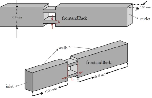
A throttle geometry was chosen to model cavitation as shown in Figure 3.13. Geometry of the domain is produced regarding the paper of Medrano et. al. [26]. As a common design in literature validation and verification studies were conducted in this geometry.
Figure 3.13: Geometry and boundary conditions of throttle configuration The configuration of this geometry is produced to investigate the effect of aspect ratio. Variations of this geometry is obtained by changing hand L which are also shown in 3.13. All of the configurations and their aspect ratios are given in Table 3.4.
Table 3.4: Configurations of Single Throttle Geometry Case Number h (µm) L (µm) Aspect Ratio
1 30 100 0.03 2 30 120 0.25 3 30 150 0.20 4 30 200 0.15 5 50 100 0.50 6 50 120 0.42 7 50 150 0.33 8 50 200 0.25 9 60 100 0.60 10 60 120 0.50 11 60 150 0.40 12 60 200 0.30 13 80 100 0.80 14 80 120 0.67 15 80 150 0.53 16 80 200 0.40 17 100 100 1.00 18 100 120 0.83 19 100 150 0.67 20 100 200 0.50 21 120 100 1.20 22 120 120 1.00 23 120 150 0.80 24 120 200 0.60
To eliminate the effects of generated mesh, three different meshes are generated and compared which are all two dimensional. These meshes are shown in Figure 3.14 and their properties are given in Table 3.5. All of the mesh refinements are made with OpenFOAM itself.
Table 3.5: Total cells of the meshes Coarse Middle Fine Total Cells 258672 356442 467160 Refinement Level 1 2 3
It is seen that the results do not show a significant change between middle and fine meshes. Axial velocity profile obtained in the middle of the throttle for the
(a) Coarse Mesh (b) Middle Mesh
(c) Fine Mesh
Figure 3.14: a) Coarse, b) Middle and c) Fine meshe sizes created for single throttle configuration
Maximum difference between middle and fine meshes for velocity is calculated as % 0.310. On the other hand between Coarse and Fine meshes this value is obtained as % 1.05. It is also seen from the Figure 3.15 that the Coarse mesh is incapable of resolving the flow near the wall. However by using, the coarse mesh clock time for simulating 1 seconds of the given analysis is around 1.577E6
seconds and the same time for middle and fine meshes are 32.72E6 and 111.11E6
seconds respectively.
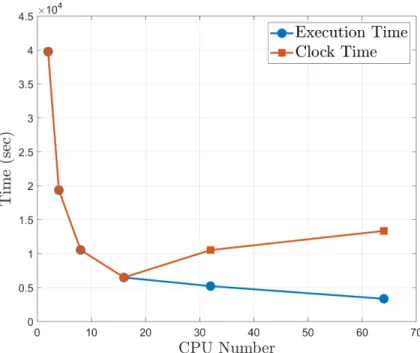
Therefore even the lowest cost in terms are obtained in the coarse mesh, op-timized accuracy and cost is obtained by middle mesh configuration. So, middle mesh refinement level will be used for the rest of this work. Also, a CPU study was conducted to determine the optimal number of cores for the analysis with the middle mesh. It is seen that CPU time drops around 16 cores and increases above this number of cores. CPU time and core number relation is given in the
Figure 3.15: Axial velocity profiles for coarse, middle and fine meshes in the throttle
Table 3.6: Total cells of the meshes
CPU Number Execution Time (sec) Clock Time (sec)
2 39758 39781 4 19350.7 19360 8 10545.6 10552 16 6484.23 6493 32 5214.28 10522 64 3352.93 13352
Regarding these values, for around 35000 cells 16 cores are used both for the throttle geometry and the other geometries which will be described in the upcoming sections of this chapter.
3.2.2
Double Channel Geometry
Regarding the single channel throttle geometry, a double channel geometry was produced for investigation of multiple channel interaction. With this way, inter-action of two jets are investigated. Geometry and is shown in Figure 3.17. h is 60 µm and L is taken as 100 µm.
ge-A grid with 2 levels of mesh refinement is again used. Produced mesh and its size is given in 3.18.
Figure 3.18: Grid of the double throttle channel geometry
3.2.3
Triple Channel Geometry
In addition to the double channel geometry, a triple channel geometry was inves-tigated too. This geometry and its dimensions are shown in Figure 3.19.
The main consideration for designing this channel is to see the cavitation behaviour when there are multiple jets that interact each other inspired from the geometry of the Schneider et al. [18]. In other words to see the effect of increasing channel numbers. A grid with 2 levels of mesh refinement is again used. Produced mesh and its size is given in 3.20.
Figure 3.20: Grid of the triple channel geometry
3.2.4
Nozzle Inspired Channel Geometry
3.2.4.1 Smaller to Larger Cross Section
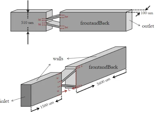
To see the effect of changing cross sectional area in the throttle part, a nozzle inspired geometry was produced. With this way the aim is to see the the effect of varying inlet and outlet area. Dimensions and the geometry are shown in Table 3.7 and Figure 3.21, respectively.
Table 3.7: Dimensions of the Geometry Dimensions (µm)
he 162 hi 60 w 225
Figure 3.21: Geometry and boundary conditions of nozzle inspired channel ge-ometry
A grid with 2 levels of mesh refinement is again used. Produced mesh and its size is given in 3.22.
Figure 3.22: Grid of the nozzle type channel geometry
3.2.4.2 Larger to Smaller Cross Section
Regarding the previous geometry, a geometry having a larger cross section than its outlet is formed basically by reversing the one shown in 3.21. Since it has the same dimensions of the previous section, grid was kept constant.
3.2.5
Double Inclined Geometry
3.2.5.1 Smaller to Larger Cross Section
Another design was created with double inclined channels. The main aim of this geometry to investigate the non-parallel jet interactions unlike the others. Created geometry is shown in Figure 3.23.
Figure 3.23: Geometry and boundary conditions double inclined channel geome-try
Dimensions labelled in 3.23 are given in Table 3.8.
Table 3.8: Dimensions of the Geometry Dimensions (µm)
he 60 hi 60 w 143.9
Chapter 4
Calculations and Simulation
Results
In this section, CFD results of the cavitation simulations with the previously discussed geometries and their related computations are given to investigate the behavior of cavitating flows. Several different coefficients and parameters critical for cavitation such as discharge coefficient and cavitation number are calculated as part of the investigation. With each geometry, analysis methodology proposed in Chapter 3 was used with 6 different input total pressure values given in 2.3. Used values are shown in Table 4.1.
Table 4.1: Measured Properties in the Set-up Input Pressure at Flow Rate Velocity Total Pressure
Point 1 (P a) (m3/s) (m/s) (P a) 100000 1.779e-08 0.3351 185250.019 200000 3.018e-08 0.5684 281283.118 300000 4.112e-08 0.7744 377825.604 400000 5.120e-08 0.9643 474677.594 500000 6.069e-08 1.1432 571746.932 600000 6.975e-08 1.3137 668978.537
4.1
Single Channel Throttle Geometry
In this section firstly the flow coefficients will be discussed then simulation results will be presented.
4.1.1
Coefficient Calculations
Several calculations and steps are taken in order to characterize the flow. As a result of these calculations; vena contracta location, contraction, velocity and discharge coefficients are obtained.
Vena Contracta
There are different parameters that defines the behavior of cavitating flows. As a start, vena contracta location is found. Vena contracta is described as the lo-cation with jets smallest area, highest velocity and the lowest pressure [39, 40]. It shows Representation of the vena contracta is shown in Figure 4.1 below.
Figure 4.1: Representation of Vena Contracta
Position of vena contracta shows variety for different channel widths and lengths. In this manner 4.2 shows the change of the location with respect to
increasing channel width for same Reynolds number. Also the effect of the chan-nel length is shown in 4.3. Two parameters are generated for these investiga-tions which are β as the ratio between the width of the throttle and the channel (β = h/510) and A as the aspect ratio of the throttle (A = h/L). Since the location of vena contracta is related to the geometry, different flow rates are not investigated.
(a) Throttle with β = 0, 12 and A=0,6
(b) Throttle with β = 0, 16 and A=0,8
(c) Throttle with β = 0, 20 and A=1,0
Figure 4.2: Location of vena contracta for different channel types) a) β = 0, 12 and A=0,6, b) β = 0, 16 and A=0,8 and c) β = 0, 20 and A=1,0
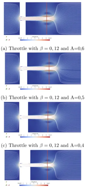
(a) Throttle with β = 0, 12 and A=0,6
(b) Throttle with β = 0, 12 and A=0,5
(c) Throttle with β = 0, 12 and A=0,4
(d) Throttle with β = 0, 12 and A=0,3
Figure 4.3: Location of vena contracta for different channel types) a) β = 0, 12 and A=0,6, b) β = 0, 12 and A=0,5 and c) β = 0, 12 and A=0,4 d) β = 0, 12 and A=0,3
As it is seen in Figure 4.2 and 4.3, channel width is the main driving parameter of channel geometries and on the contrary, channel length has no effect on the location of vena contracta.
Effect of the Reynolds number for the same channels are also investigated. Fig-ure 4.4 shows the behaviour of vena contracta location with respect to Reynolds
(a) Re=25
(b) Re=43
(c) Re=58
Figure 4.4: Location of vena contracta for different Reynolds numbers a) Re=25 b) Re=42.6 and c) Re=58
Contraction Coefficient
Contraction coefficient is a parameter to express the relation between the ori-fice geometry and the flow of the oriori-fice. It is defined as the ratio between the areas of the flow at vena contracta to the area of the channel. Equation 4.1.1 shows this relation between channel width and vena contracta [41].
Cc=
Area of the f low at vena contracta
Area of the channel (4.1.1.1)
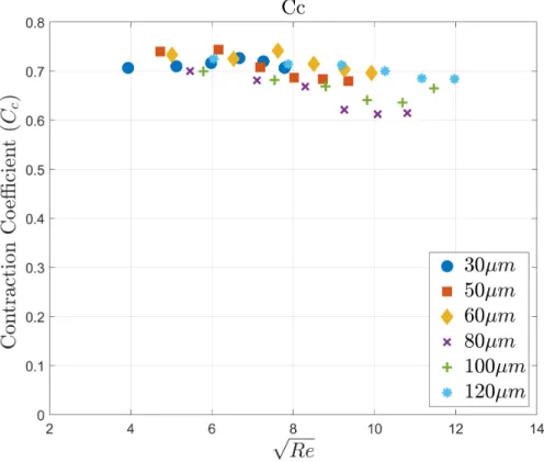
As both the area of the flow at vena contracta and channel width showed variety, contraction coefficient differs with respect to channel area. Results for channels are given with respect to the square root of Reynolds Number in the Figure 4.5.
Figure 4.5: Contraction Coefficient with respect to the Square Root of Reynolds number
Table 4.2: Contraction Coefficient Results for single throttle geometry Input Pressure (P a) 30 50 60 80 100 120 Average
100000 0.707 0.740 0.733 0.700 0.700 0.725 0.717 200000 0.710 0.744 0.725 0.681 0.682 0.714 0.709 300000 0.717 0.708 0.742 0.669 0.669 0.713 0.703 400000 0.727 0.687 0.715 0.621 0.641 0.700 0.682 500000 0.720 0.684 0.703 0.613 0.636 0.685 0.674 600000 0.707 0.680 0.697 0.615 0.665 0.684 0.675 Average 0.716 0.713 0.724 0.657 0.707 0.684
Average value is around 0.7 for the contraction coefficient and it can be con-cluded that as the pressure at the inlet increases contraction coefficient is de-creasing.
Discharge Coefficient
Discharge coefficient is defined as the ratio between actual flowrate of a throttle to the theoretical one [42]. There are several different ways to calculate it, for common type of valves, orifices etc. it is pre-determined by experiments [42, 43]. From the definition the relation between the coefficients are stated as follows [42];
Q = AV = CcCvA0Vi = CdA0Vi (4.1.1.2)
where A is the area of vena contracta, A0 is the area of the throttle and Vi is the
velocity at vena contracta. However, there are other methods for determining the discharge coefficient. It is driven from the Bernoulli equation its relation to the flow rate is written as [26];
Pin− Pout = 24µL W H3(1 + H W) 2Q + ρ 2C2 d Q2 h2H2 (4.1.1.3)
entrance section, Q is the flow rate and Cd is the discharge coefficient. However,
this equation does not satisfy certain conditions.
Then the relation regarding the discharge coefficient is simplified to the fol-lowing Equation 4.1.1 [26]; 1 Cd = 1 Cc − h W (4.1.1.4)
However, this equation does not satisfy conditions. As Reynolds Number gets smaller, effect of the viscous forces gets dominant and the previous equations can not model it [44, 45]. For those cases, in his book H.E. Merritt tabulates the discharge coefficients of short tube orifices as follows; For DhRe
L > 50 Cd = [1.5 + 13.74(L/DR) 1 2] −1 2 (4.1.1.5) For DhRe L < 50 Cd= [2.28 + 64(L/DR)] −1 2 (4.1.1.6)
For lower Reynolds numbers such as Re < 10 equation can be directly written as a function of Reynolds Number;
Cd= δRe
1
2 (4.1.1.7)
where δ is laminar flow coefficient related to the geometry. In addition to this one, Wu et. al. successfully derived the equation in terms of Reynolds Number for higher Reynolds Numbers too. The equation is given in 4.1.1 [46].
For those purposes, Reynolds Numbers for the single throttle channel geome-tries is given in Table B.0.3 in Appendix B.0.3. Discharge coefficient results obtained from the simulations are given in 4.6.
Figure 4.6: Discharge Coefficient with respect to the Square Root of Reynolds number
These results are then compared with the values obtained from equation that Wu et. al. derived. Results of channels with with of 30, 80 and 120 µm are given in 4.7, 4.8 and 4.9. Results of other channels are given in B.0.1. Even though the values are clustered in a small range, it is observed that as the Reynolds numbers increase the values are decreasing.
Figure 4.7: Discharge Coefficient of β=0,06 and A=0,3
Figure 4.9: Discharge Coefficient of β=0,24 and A=1,2
Percentage errors are calculated between the equation of Wu et. al. [46] and CFD simulations. The results are given in Figure 4.10. It is seen that the lowest error value is obtained for 100 µm width channel. In terms of the input pressures lowest error values are obtained for 5 and 6 bar simulations. Table 4.3 provides values for each case.
Table 4.3: Percentage Errors for Discharge Coefficient in Single Channel Geom-etry
Input Pressure (P a) 30 50 60 80 100 120 Average 100000 5.654 6.705 7.304 2.364 5.517 10.611 6.359 200000 2.330 11.863 11.191 2.508 3.829 10.333 7.009 300000 4.937 8.442 13.833 2.493 1.988 9.785 6.913 400000 9.531 4.486 10.253 4.057 2.088 8.042 6.410 500000 7.600 5.447 8.738 5.409 1.927 5.980 5.850 600000 9.056 4.276 7.260 5.202 1.706 5.139 5.440 Average 6.518 6.870 9.763 3.672 2.843 8.315
Figure 4.10: Percentage Error in Discharge Coefficient calculations Velocity Coefficient
After the calculations of contraction and discharge coefficients velocity coef-ficient is calculated from the definition. Obtained results are given in Figure 4.11.
It is observed that as the Reynolds numbers increase the values are clustering near 1, yet the maximum coefficient calculated is 0.99 at most. Besides coefficients several different aspects in the design of throttle are investigated. These will be discussed in the upcoming sections.
Figure 4.11: Velocity coefficient results for single channel Geometry
4.1.2
Effect of Input Pressure
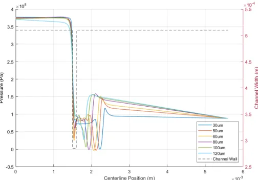
As it is discussed previously, variation in input pressure changes the location of vena contracta, this effect can also be seen from the change in pressure along the center line of the channel. This effect is shown in Figure 4.12. Velocity graph along the same center line is given in B.0.2.
Location of the lowest pressure point also affects the phase change. Alpha contour of the channel with 60 width in Figure 4.13 shows the variation in the formation of bubbles in different input pressure values (ratio of fluid volumes as 1 being incompressible and 0 being compressible).
(a) Place of the centerline
(b) Pressure Changes for different channel thicknesses
Figure 4.12: Pressure change along the channel at t=0.00013s for different inlet pressures
Figure 4.13: Phase change at different input pressures
4.1.3
Effect of Channel Thickness
To investigate the effect of channel thickness in cavitating flows, firstly the pres-sure change over the channel is investigated. For the same time step and same inlet total pressures, 4.14 shows the difference in pressure change over the center line of the channel.
When channel thickness is changed the alpha contour varies as it is shown in Figure 4.15 for a given inlet pressure of 3 bars. As the thickness increases, the time that vapour bubble forms changes regarding the velocity and pressure drop. However, decreasing it too much will also increases the friction losses. Therefore at 50 and 60 µm channels vapor bubbles tend to occur faster.
Figure 4.14: Representation of the Flow in the Experimental Set-up
4.2
Double Channel Geometry
Double channel geometry is created by multiplying a single channel. Jets created for each channel is identical with the single channel geometry until they collide with each other. After the interaction flow becomes completely chaotic. In this manner, velocity contour changing with respect to time is given in Figure 4.16 for the simulations with inlet pressure of 3 Bar. Pressure contour is given in Section B.0.4.1.
Figure 4.16: Velocity Contour with Respect to Time for Double Channel Geom-etry
As it is seen, flow is symmetrical since jets are not interacting with each other at t=0.00035 s. Then when two jest interact with each other flow pattern becomes random and chaotic as it is expected
Pressure drop along the center line of each channel is investigated for the 0.0005 second. Before any disturbance all pressure variations are equal. At 0.0005 however, jets start to collide and create chaotic variations.
Figure 4.17: Pressure Change in Channels in Double Channel Geometry Bubbles on the other hand starts to occur before that time since the pressure drop reaches below the vapor pressure beforehand. Related alpha contour is given in Figure 4.18.
Figure 4.18: Alpha Contour with Respect to Time For Double Channel Geometry
4.3
Triple Channel Geometry
Triple channel geometry is created by placing three equal sized channels with equal distances to each other. Similar to the double channel geometry jets created for each channel is identical with the single channel geometry until they collide with each other. After the interaction flow becomes completely chaotic. In this manner, velocity contour changing with respect to time is given in Figure 4.19 for the simulations with inlet pressure of 3 Bar. Pressure and alpha contours are given in Section B.0.4.1.
As it is seen, flow is symmetrical until jets interact with each other at a previous time step than the double channel geometry. This behaviour is expected since the distance between the channels are narrower than the double channel geometry. Then when jets interact with each other flow pattern becomes random and chaotic again.
Figure 4.19: Velocity Contour with Respect to Time for Triple Channel Geometry
Pressure drop along the centerline of each channel is investigated for the 0.0005 second again.
Bubbles on the other hand starts to occur before that time since the pressure drop reaches below the vapour pressure beforehand. Related alpha contour is given in Figure 4.21.
Figure 4.20: Pressure Change in Channels in Triple CHannel Geometry
4.4
Nozzle Inspired Channel Geometry
4.4.1
Smaller to Larger Cross Section
Nozzle inspired geometries are created with increasing or decreasing the initial inflow area at the throttle region. As it is expected, when the exit area is smaller than the inlet area flow tends to speed up and opposite happens when the exit area is larger. In this manner, velocity contour changing with respect to time is given in Figure 4.22 for the simulations with inlet pressure of 3 Bar. Pressure and alpha contours are given in Section B.0.4.1.
Figure 4.22: Velocity contour with respect to time for nozzle type channel geom-etry
In this manner, velocity contour of the mirrored geometry is given in 4.23. Different characteristics of the jets can be seen at t=0.00035 clearly. Jet in Figure 4.23 goes further than the one given in 4.22.
Figure 4.23: Velocity contour with respect to time for nozzle type channel geom-etry
To compare the phase change behaviour pressure changes along the centerline of both channels are presented in 4.24. It is seen that in larger to smaller section geometry, pressure drop is higher as it is expected.
Figure 4.24: Pressure changes along the centerline of the nozzle inspired geome-tries
4.5
Double Inclined Geometry
Double inclined geometry is formed by two channels placed inclined to each other with 80.06 degrees as shown in Figure 4.25.
Figure 4.25: Angles in between channels
Firstly the jets are investigated regarding the velocity contours for 3 Bar inlet pressure given in Figure 4.26. It is seen that again two symmetrical jets are flowing until they distort each other.
Alpha contour of the given time steps are given in Figure 4.27 below. Fastest phase change is observed for this design due to the flow direction.
Corresponding pressure contour and vectors along the streamline are given in Section B.0.4.4.
Figure 4.26: Velocity contour with respect to time for nozzle type channel geom-etry
Chapter 5
Experimental Set-up, Fabrication
and Results
Experimental up was built to observe the cavitation phenomena. This set-up includes several parts such as the microfluidic devices whose geometries were given in Chapter 3, the pressure pump that is the main drive for fluid flow and a high speed camera for capturing the motion. In this chapter, components of the experiment set up and fabrication method will be explained. Lastly, the visuals obtained from the set-up is presented.
5.1
Set-Up
The set up includes several components which are listed below;
• A pressure pump • Pressure regulator • Air drier
• Microfluidic chip • Fluidic connectors • High speed microscope • Pressure supply
The listed items are connected with each other as it is given in Figure 5.1 below.
5.2
Fabrication of Microfluidic Chips
Microfluidic chips in which the cavitation was investigated were fabricated with photolithography technique. Among the different types of polymers, poly-dimethylsiloxane (PDMS) was used to create the chips with the conventional softlithography.
The procedure starts with creating a SU-8 (negative photoresist) mold that consists the desired chip geometries. Then using the mold the chips were fabri-cated from the PDMS and bonded to glass. The detailed procedure is as follows; 1) First step for the process is cleaning a 4 inch silicon wafer with acetone, isoproponal and DI water respectively. Then it is dried completely with first nitrogen gun and afterwards by putting it into the oven at 120◦C for 5 minutes to vaporize the moisture remaining on the surface.
2) As an initial base layer, wafer is coated with SU-8 2005 by using spin coater. Spin parameters are given in Table 5.1. Chemical information and parameters of SU-8 2005 is set regarding the data sheet provided [47].
Table 5.1: Spin parameters for base layer
Step Velocity (rpm) Acceleration (rpm/s) Time (s)
1 500 100 25
2 200 200 40
3) The wafer is prebaked on a hot plate with 65◦C, 95◦C and 65◦C step by step with 2, 4 and 1 minutes respectively. When the heating is over wafer is cooled down to room temperature.
4) Later, the wafer is exposed to UV light with the settings provided below by using an empty glass mask.
- Manual top side - Contact Mode: Soft Contact - Separation: 100 µm
- Resist thickness: 2 µm
- Exposure intensity: 120 mJ/cm2
5) Sample is baked again at 65◦C, 95◦C and 65◦C on hot plate for 1, 3, and 1 minutes respectively and left for cooling down to room temperature.
6) Next step is coating the wafer with SU-8 2050 with spin coater. The pa-rameters used for this step is provided in Table 5.2 below [48].
Table 5.2: Spin parameters for main layer
Step Velocity (rpm) Acceleration (rpm/s) Time (s)
1 500 50 40
2 2200 300 35
7) Wafer is baked again at 65◦C, 95◦C, and 65◦C on heaters for 3, 8, and 2 minutes respectively and then left for cooling to the room temperature.
8) Later, the wafer is exposed to UV light with the settings provided below and using the mask created before the process. Design of the mask consists of the desired chip geometries and it is given in C.
- Manual top side
- Contact Mode: Soft Contact - Separation: 200 µm
- Mask thickness: 2.3 mm - Sample thickness: 0.5 mm - Resist thickness: 2 µm
- Exposure intensity: 230 mJ/cm2
9) Following the spin coating process, wafer is baked at 65◦C, 95◦C and 65◦C on heaters for 3, 8, and 2 minutes respectively and then left for cooling down to the room temperature.
11) When the geometries are formed the wafer is washed with DI water. 12) Wafer is dried with a nitrogen gun until there are no water bubbles left and then the PDMS mixture with its curing agent is poured on the wafer.
13) To eliminate the bubbles inside the PDMS mixture, the vacuum pump is used.
14) When there are no bubbles inside the solution, it is put on the oven at 80◦C for 30 minutes to harden PDMS.
15) As the PDMS hardens, it is peeled off from the master mold and cut into the pieces forming the chips and tubing holes are also opened.
16) Following the cleaning procedure of both PDMS mold and the glass, they are bonded to each other with plasma cleaner.
17) As a final step, tubings are connected to the chips with epoxy. Steps that are taken during this process is schematically shown in 5.2.
Chips that are fabricated with this method are investigated under the micro-scope. Figure 5.3 shows the sample produced.
Figure 5.2: Photolithography technique to produce microchips with negative pho-toresist
5.3
Experimental Results
From the set-up that is previously explained, by using high speed camera tak-ing 8-16 frames per second visuals of the cavitattak-ing flows are taken. It is seen that for lower input pressure values, flow does not encounter any phase changes. Representation of these flows are given in Figure 5.4 below for single throttle channel in 3 bars. It is shown that these flows are creating regular steady state flow behavior.
Figure 5.4: Steady flow in 30 micron width channel with 3 bars input pressure This behaviour does not change its characteristics with any of the designs pre-described. For example Figure 5.5 shows the same steady flow with nozzle inspired geometry.
As the input pressure is increased however, flow characteristics change like it is predicted in the simulations. For example for higher pressure values bubbles tend to occur and fade away. Around 4 and 5 bars these random bubbles start to occur as it is also predicted in the simulations early time steps. For 30 micron width single throttle channel the moment of the bubble occuring is captured and marked in 5.6. More visuals are provided in D.
Figure 5.6: Vapour Bubble in the 30 Micron Channel
For around 5 and 6 bars, bubbles given in Figure 5.6 becomes multiple and resembles the simulation more. This similarity is highlighted in Figure 5.7 as both the CFD and the experiments have multiple initial low density zones.
For the higher velocities these formation of bubbles increase however since the flow is highly chaotic bubbles occur and disappears suddenly. Visual of this kind of a moment is given in Figure 5.8 with the similar simulation result.
Figure 5.8: Symmetrical Low Density Zones in Simulation and Experiments Cavitation behaviour is also investigated using latex beads, which are carboxylate-modified polystyrene fluorescent yellow-green, to compare the ex-perimental results with simulation.
In Figure 5.9a, the region of vortex is clearly seen at the initial time steps and the movement of the vortex region is shown in Figure 5.9b.
(a) Vortex Region
Then as the time passes, the cavitation zone becomes larger which is shown in Figure 5.10.
Figure 5.10: Cavitation Zone
Symmetrical formation of low density zones where the simulation also predicts is given in Figure 5.11.
Figure 5.11: Symmetrical Low Density Zones
Throughout these experiments several parameters are controlled for the accu-racy of the processes. Firstly, qualities of the chips which are fabricated by using
curing agent for every trial. Also, as the length of the tubing is important to reduce the friction and import a higher velocity fluid, the length of the tubings are also measured equally and implemented in the same ways for each chip. In addition, fluid is always used from the sealed tube providing the same fluid con-stantly to the system. Identical situation applies for the pressurized gas that is used for the pressure pump, also the pressure regulator is kept constant at its possible maximum condition always to prevent any input pressure changes.
Also, de-gasification was tried by placing the water in a vacuum chamber for 24 hours. Similar pattern is observed on our case due to our set-up as it is seen in Figure 5.12 below.
Figure 5.12: Cavitation Bubble with Degasified Water
However, even the experimental results show great resemblance with the sim-ulations, certain upgrades can be applied for better quality. These improvements that will increase the visual capability and data quality will be discussed in 6.
Chapter 6
Conclusion and Future Work
Throughout this study, several geometries and test cases were produced to in-vestigate the behavior of cavitating flows. To simulate the flow, measurements are conducted and implemented in the open source software OpenFoam with the boundary conditions that are verified previously.
Several different cases were run for single throttle channel geometry such that both the effect of thickness of the channel and the effect of input pressure on the cavitation is investigated. Cases with varying input pressures were also generated for other geometries.
It is seen that increasing the Reynolds Number and decreasing the channel width shifted vena contracta point towards left. On the other hand, increasing the channel width moved it towards right. It is also observed that the channel length does not have any significant effect on the vena contracta point. As the vena contracta point shifts towards right it can be said that the bubbles are forming at a previous time step.
However, decreasing the channel width too much also results of higher friction and dominancy of viscous forces. Therefore, it is not always correct to say that as the channel width decreases bubbles form faster.