Safety stock placement for serial systems under supply
process uncertainty
Bengisu Urlu1 · Nesim K. Erkip2
Published online: 1 January 2020
© Springer Science+Business Media, LLC, part of Springer Nature 2020
Abstract
In this study, we address safety stock positioning when demand per period is a known constant but supply is uncertain. The supply is either available or not available, while the setting is that of a periodically reviewed, serial system following a base stock pol-icy. Each stage is allowed to operate according to the guaranteed or stochastic service model. We use a Discrete Time Markov Chain model for expressing the expected on-hand inventories for each stage, along with other terms of interest, as a function of policy parameters determined by a given service level requirement for the end product. Exact models are constructed for single-stage and two-stage systems. As the number of states for a two-stage system grows exponentially, we propose an approximation for expressing the effect of the input stage using a single parameter. A generalization for the approximation is provided for a multi-stage problem. Computational evaluations of the approximation, as well as numerical comparisons of different cases, are presented.
Keywords Inventory management · Safety stock positioning · Supply uncertainty · Serial systems
1 Introduction
The safety stock placement problem involves determining the right amount of base stock in each stage, to ensure the required service level or the lowest expected cost. A stage may have a stock of finished goods as well as work-in-process inventory to
Bengisu Urlu started conducting this research at Bilkent University. She continued working on it at Eindhoven University of Technology, and finalized at INSEAD.
* Bengisu Urlu
[email protected] Nesim K. Erkip [email protected]
1 Technology and Operations Management, INSEAD, Fontainebleau, France 2 Department of Industrial Engineering, Bilkent University, Ankara, Turkey
enable possible production realization. There are many approaches to solve the stock
placement problem: Song and Zipkin (2003) and Atan et al. (2017) present
com-prehensive reviews of undertaken studies, especially on assembly systems; Axsäter
(2003) examines divergent systems; Inderfurth and Minner (1998) study service
concepts in such systems; and Graves and Willems (2003) investigate more general
multi-echelon systems. Among safety stock placement approaches, we use the two
regimes presented by Graves and Willems (2003); namely, the stochastic service
model (SSM) and the guaranteed service model (GSM). In the SSM, stock place-ments at each stage are performed according to a function of the stochastic delay from upstream stages. In the GSM, each stage ensures that it can meet its require-ment for the next stage by committing to a maximum service time (Graves and
Wil-lems 2003). In these models, it is assumed that supply is always available at each
stage and at each period of operation.
Supply uncertainty refers to supply disruptions, which may be due to operational inefficiencies as well as intentional or unintentional human actions; hence, it has
sev-eral forms, as described in Snyder et al. (2016). Yield uncertainty covers the cases
where the quantity delivered by a supplier or the amount produced by a manufac-turing process is a random variable that depends on the order quantity. Capacity uncertainty, in contrast, covers the cases where the supplier’s delivery capacity or the company’s manufacturing capacity is a random variable that is generally independ-ent of the order quantity. Transportation time uncertainty occurs due to the stochastic nature of transportation time. Finally, process uncertainty considers the variability of the production processes. In a way, it is similar to yield uncertainty, but one may end up with no production as a result of process variability. There are many studies
on delineating supply uncertainty structures. Silver (1976) defines supply uncertainty
by allowing the quantity received to be a random variable and a random proportion
of the quantity ordered. Shih (1980), Ehrhardt and Taube (1987), and Henig and
Ger-chak (1990) also regard uncertain supply as a random multiple of the quantity
req-uisitioned. Parlar and Berkin (1991) view supply uncertainty as a situation in which
supply is either available or unavailable for a random duration in a continuous review
environment. Similarly to our base model, Güllü et al. (1997) define supply
uncer-tainty as supply being either fully available or completely unavailable according to
some probabilities, in a periodic review setting. Güllü et al. (1999) extend the same
idea and regard supply uncertainty as supply being fully available, partially available, or completely unavailable according to some probabilities. Other pertinent models
are described in two review articles by Yano and Lee (1995) and Snyder et al. (2016).
Another related research area is the analysis of tandem queues with finite buff-ers and unreliable machines. In this area, most of the traditional literature has been devoted to modeling and analysis of such production systems, with the central issues being performance analysis and computability. More recently, studies have considered an objective function that incorporates system performance and the cost of buffers between stages (usually of an automated production system). There is an analogy between this set of problems and the stock positioning problem: Position-ing stocks can be considered as holdPosition-ing buffers in tandem queues with finite buff-ers. The distinction in the literature usually comes in the environmental description of the problem (e.g., type of processes, demand distribution, service distribution,
etc.), as well as in the objective function. The objective function of a typical serial inventory system considers holding costs which are functions of the stage, whereas in the majority of the tandem queue literature only a constraint on the total buffer usage is considered, assuming equal cost buffers. Nevertheless, there are important overlaps in the analytic approaches, especially when the distributions in question are identical. A recent review of the so-called buffer allocation problem can be found in
Weiss et al. (2019). As stated in that review, one area authors claim is “insufficiently
captured” by the literature is when there is uncertainty in the supply process, and this is the aspect we aim to study in our current work. There are numerous stud-ies on tandem queues, but here, we refer to a more related and recent set of studstud-ies that consider solution algorithms for the buffer space allocation problem (Gershwin
and Schor 2000); lines operated with given policies (Wu et al. 2017;
Liberopou-los 2018); and, lines with tandem queues and unreliable machines (Lee et al. 2017,
2018).
The main purpose of this research is to consider supply uncertainty for the safety stock placement problem. Our main motivation stems from serial systems, repre-senting an important special case of assembly systems. Serial systems usually oper-ate on a just-in-time basis, meaning that suppliers are expected to deliver in small lots to the next stage and finally to the equipment manufacturer, every day or even more frequently. The equipment manufacturer performs final assembly, which is well-planned, and practically there is no uncertainty in the desired throughput of the assembly line. Moreover, one can claim that the quantity produced per day is a constant, as a result of the assembly line balancing efforts. It is quite common to observe certain suppliers’ inability to ship every day, motivating an all-or-nothing type of supply uncertainty. We call this type of uncertainty “process uncertainty”, usually resulting from an equipment failure or failure of the second-tier suppliers to supply the necessary input. Note that this structure of process uncertainty is also
well studied in tandem queue literature (for examples, see Lee et al. 2017, 2018).
What is interesting about the problem is that process uncertainty structure brings in the necessity of safety stock placement in different stages, although demand is not stochastic. A limited number of studies incorporate both supply and demand
uncertainty in the same modeling environment. Bollapragada et al. (2004a, b) model
the supply process allowing for backlogs but limiting their duration, similar to a restricted GSM approach.
We consider a periodic review system in which each stage has an order-up-to point. Demand per period is Q units, deterministic and known. We assume a supply uncertainty structure where supply is either available or not available, as described
by Güllü et al. (1997). The structure, depicted by Bernoulli-type stages, has been
considered by the tandem queues literature as well. For example, Diamantidis and
Papadopoulos (2004) offer a dynamic programming approach for buffer allocation,
and Naebulharam and Zhang (2014), Lee et al. (2017, 2018), address waiting
time-restricted products for performance evaluation. Hence, a stage may have sufficient work-in-process to work on, but as a result of process uncertainty, it may not be able to produce. Additionally, if no work-in-process is available, the stage will not be able to produce, following the “starvation” characteristic described mostly by the tandem queue literature. If there is sufficient work-in-process and production is realized,
then any quantity to bring the stocks to the order-up-to point can be produced. In other words, there is no capacity restriction. Hence, following these characteristics, a stochastic delay term can be defined for items to be available for the next stage. Therefore, the core of the problem is to reflect the stochastic characteristics of the supply uncertainty problem combined with the characteristics of the safety stock placement models.
To fulfill our research purpose, we restrict our analysis to serial systems. Graves
and Willems (2005), Hua and Willems (2016a, b) present evidence for the
impor-tance of analyzing a two-stage serial system. Gavirneni (2004) describes a chip
manufacturer with a four-stage serial system. Although the supply chain of the chip manufacturer is far more complex, the author identify a small number of suppli-ers responsible for inefficiencies in the operations, and hence it can be reduced to a serial system. Our objective in this research is to obtain exact (and if possible explicit) terms for the considered serial system. We use the two regimes introduced (SSM and GSM) as possible stock placement models, in addition to implementing a supply uncertainty structure in which supply is either fully available or not available at all. Then, we model the system as a Discrete Time Markov Chain (DTMC).
Our main contribution is modeling the stock placement problem in serial sys-tems with supply uncertainty given the presumed structure. Contrary to the avail-able literature, we allow different stages to operate with different service regimes, each stage following either the SSM or the GSM. We compare two-stage systems based on expected safety stock costs, and further compare SSM and GSM regimes. We propose an approximation method as the number of states in the DTMC model grows exponentially.
The paper is organized as follows. Section 2 provides necessary background
information. In Sect. 3, we consider single-stage and two-stage problems,
operat-ing with the GSM or the SSM. In Sect. 4, we present the approximation scheme and
generalization of the approximation to a multi-stage problem. Our computational
experiments for the two-stage models and comparisons appear in Sect. 5. Finally,
in Sect. 6 we conclude and offer possible generalizations and other extensions for
future work. 2 Background
2.1 Supply uncertainty
In Güllü et al. (1997), an inequality that provides the optimal number of periods
(K) to consider during which the cumulative demand is equal to optimal order-up-to level is derived. In our research, we focus on the special case of a similar problem with infinite time horizon. Note that K stands for the number of periods of demand and in our case the order-up-to level is KQ. Additionally, the right side of the ine-quality is represented by a service level definition rather than costs, following the
service-level definition made by Silver (1976), and used by Graves and Willems
(2003). As a complementary explanation, we can say that each value of K
2.2 Approaches to safety stock placement
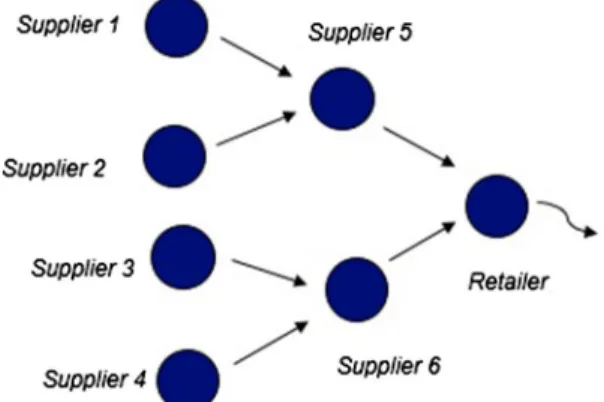
Graves and Willems (2003), consider two regimes of the safety stock placement
problem, referred as the guaranteed service model (GSM) and the stochastic
service model (SSM). They consider the general environment shown in Fig. 1.
Note that the aim is to characterize the replenishment times, given that a stage might have multiple unreliable upstream suppliers that might also have unreliable suppliers.
Each regime structure allows for writing an approximate expression of the expected replenishment times. The system operates according to an order-up-to
policy where the base stock is given in Graves and Willems (2003). Using these
replenishment times, safety stocks can be computed. The total expected safety stock cost can be found and used for performance evaluation for a given set of service level targets (or safety factors) in each stage in an optimization context. Finally, for any regime the purpose is to eventually come up with safety stock terms for each stage to minimize total expected cost of safety stock of the system to satisfy a service level target of the end-product. Note that the safety factors of all stages are decision variables.
Under the SSM regime, Graves and Willems (2003) assume that at most one
supplier is allowed to stock out per period, and delay is equal to this supplier’s processing time. Thus, they represent replenishment time for a stage as a func-tion of the processing time of the current stage added to the expected value of the processing time from the predecessor stage, causing a stock-out. The probabilities
used to compute expectations are not exact and are taken from Ettl et al. (2000).
Moreover, demand over the net replenishment time is assumed to be normally dis-tributed with a mean and a standard deviation, that are derived once the expected replenishment time is determined. Note that if we follow the supply uncertainty structure specified in the previous subsection, the implementation of the SSM at
Stage j corresponds to finding Kj , and hence the order-up-to level is KjQ.
When it comes to the GSM, the challenge is to determine the maximum ser-vice time given a safety factor and a demand upper bound. Serser-vice times are
Fig. 1 Representation of
decision variables for internal customers and exogenous input for external custom-ers. Demand is again assumed to be normally distributed and the demand upper bound can be arbitrarily set. In this case, the maximum service times of inbound and outbound stages affect the replenishment time.
In the GSM, if demand exceeds the upper bound, the available safety stock in the system will not be enough to satisfy the service time promise. Graves and
Wil-lems (2003) assume that in the case of excess demand, the amount that is above the
upper bound can be regarded as loss or outsourced to satisfy customer requirements. However, there is no additional term that represents the outsourced amount in their objective function. An approach to model the case when these assumptions are
vio-lated can be found in Rambau and Schade (2014).
Note that if we follow the specified supply uncertainty structure, the
implementa-tion of the GSM for any Stage j corresponds to finding order-up-to level KjQ , and a
maximum service time (in units of periods) promised to satisfy requirements, call it
Mj . Note that Mj>Kj because the order-up-to level economically should not exceed
the maximum number of periods designated for the guaranteed service time.
Fur-thermore, Mj= Kj means that there will be no backlog.
2.3 Statement of the problem
Following the standard literature, we can state our problem as: Minimize total expected safety stock cost over all stages subject to: service level constraint for the end product
Given the supply uncertainty structure presumed and supporting two regimes of ser-vice (the SSM and the GSM), in the rest of the subsection we detail the above prob-lem statement.
Stages are numbered in a decreasing way, Stage 1 defines the final stage. For each stage we have at most two variables to decide: Kj is the order-up-to level, and Mj is
maximum service time defined in Graves and Willems (2003) (note that if Stage j is
operated by the SSM regime, Mj becomes infinity).
We depict the order-of-events in Fig. 2 and present the description below. Note
that all quantities are integer multiples of Q.
• We start any period for Stage j by receiving whatever was sent by Stage j + 1
lead-time periods ago. Anything received is added to RMj,“raw material” for Stage j (the input needed to produce at Stage j).
• Stage j observes its finished goods inventory, FGj.
• If FGj>0,
– demand for Stage j − 1 is satisfied from stock and arrives at the downstream stage after the appropriate lead time.
– FGj is reduced by one.
– Stage j applies order-up-to production using Kj . Maximum production is limited by the amount of raw material inventory on hand, RMj.
• If RMj>0 and production is successful, update RMj and FGj.
• Otherwise, no change.
• If FGj≤ 0,
– demand cannot be satisfied from stock. – FGj is reduced by one.
– Stage j applies order-up-to production. Maximum production is limited by the amount of raw material inventory on hand, RMj.
• If RMj>0 and production is successful, check RMj− Kj.
– If RMj− Kj>0 , RMj− Kj units of FGj are sent to Stage j − 1 to
sat-isfy accumulated backlogs.
– Otherwise if RMj− Kj≤ 0 , RMj units of FGj are sent to Stage j − 1 ,
to partially satisfy accumulated backlogs. – Update RMj and FGj.
• If RMj= 0 or production is not successful: If Stage j operates according
to the GSM regime and a delay of Mj periods has occurred, then Stage
j outsources and sends the unit to Stage j − 1 . To account for the
out-sourced amount, the finished goods inventory is increased by one and the raw material inventory is decreased by one as it is not needed any-more. If the raw material inventory is zero, the finished goods inventory level of Stage j + 1 is increased by one (note that the finished goods inventory level of Stage j + 1 should be negative, and by subcontracting one unit we are eliminating the need for that unit).
The initial stage (the one with the largest index) is assumed to have an uninter-rupted infinite supply. Define hj as the holding cost for one finished item in Stage
j. Define E[INj] as the expected ending on-hand inventory for the finished item of Stage j (note that part of the inventory can be located at Stage j − 1 as raw mate-rial waiting for production in Stage j − 1).
Hence we can now rewrite the problem statement:
subject to:
Probability of not satisfying the demand at Stage 1 ≤ 1 - service level desired It is important to point out that expected ending on-hand inventory is safety stock plus expected demand in a period. In the next two sections, we show how we can derive the above expected ending on-hand inventory and the probability terms exactly, given Kj and Mj for all j, for single-stage and serial two-stage systems using DTMC models. Note that these terms are exact, contrary to the available literature. We also derive certain quantities of interest, expected number of backlogs, expected number of subcontracted units (0 if the stage is following the SSM regime), and expected work-in-process inventory (for Stage 1, only for the two-stage system) to be used for computational study. Furthermore, we derive the probability of Stage j satisfying the demand of Stage j − 1 on time, which we call the probability of supply
( 𝜋Sj ). This parameter is instrumental for decomposing the stages, and characterizing
service level. Note that Stage 1’s (the most downstream stage) probability of supply is equal to the service level faced by the end customer: hence it is the system’s ser-vice level. Therefore, probability of not satisfying the demand at Stage 1 is the term
for the left-hand side of the constraint for the model represented by Eq. (1).
3 Single‑stage and two‑stage problems
3.1 Single‑stage problem
To correctly reflect the characteristics of the safety stock placement models and the supply uncertainty model, we start with the simplest model, single-stage when demand is stationary and production is uncertain. We assume that the predecessor stage always supplies the needed raw-material, and hence the single-stage consid-ered is operating to satisfy the next stage. We assume that transportation time (L) is deterministic. To simplify the exposition, in the next two subsections it is presumed that transportation time is zero. Following the subsections, we generalize our results for any L.
If there is sufficient inventory at the beginning of a period, the next stage’s demand is satisfied immediately. However, if there is no inventory and production cannot be realized, there is a delay. Hence, the delivery delay faced by the lower stage is reflected as the replenishment time. Note that having no inventory implies that there have been some consecutive periods of unsuccessful production.
Therefore, the replenishment time is a random variable, 𝜏 . Using the all-or-nothing supply, 𝜏 follows a geometric distribution for the SSM regime (or a truncated geometric (1) min Kj,Mj,∀j ∑ j hjE[INj]
distribution for the GSM), where p is the probability of no production and i period
delay is faced with probability pi(1 − p).
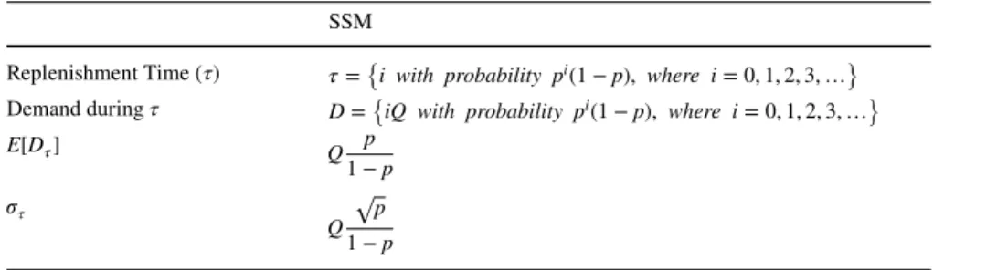
3.1.1 Stochastic service model
The demand during replenishment time also follows a geometric distribution with parameter p. The expressions for the distribution of the replenishment time, distribu-tion of demand during replenishment time, expected demand, and standard deviadistribu-tion of
demand during replenishment time are presented in Table 1.
To obtain the terms of the model, a DTMC model is used. The states of the Markov Chain are defined as the net inventory levels at the end of a period, following the order
of events structure in Fig. 2. Hence, at the beginning of the period, if possible, demand
is satisfied. After demand is satisfied, production order is placed up to the order-up-to level. For a given probability of no production, suppose the order-up-to level is given as KQ. Hence, when the replenishment time is realized as zero, the ending inventory of period t will be positive, let us say (K − n)Q . Inventory level after satisfying the demand will be (K − n − 1)Q and ending inventory of period t will again be KQ if the production is successful, since it produces up to the order-up-to level. If not, the state will remain as (K − n − 1)Q . Replenishment time will take positive values if the inventory level at the end of a period is not positive, and production is not successful for some periods. This setting is a special case of the standard birth and death process.
The transition matrix is given in “Appendix 1”, when Q is assumed to be 1 to ease the
notation.
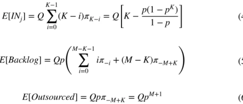
One can obtain steady-state probabilities using standard analysis where 𝜋j indicates the long-term probability that there will be j units of inventory at the end of a period. As a result, steady-state probabilities are given by
Expected ending on-hand inventory and expected number of backlogs in the system can be written as 𝜋 K−n= pn(1 − p) for n = 0, … , ∞ (2) E[INj] = Q K−1 ∑ i=0 (K − i)𝜋K−i= Q [ K−p(1 − p K) 1− p ]
Table 1 Details of the SSM for single-stage model
SSM
Replenishment Time ( 𝜏) 𝜏={i with probability pi(1 − p), where i = 0, 1, 2, 3, …} Demand during 𝜏 D={iQ with probability pi(1 − p), where i = 0, 1, 2, 3, …}
E[D𝜏] Q p 1− p 𝜎𝜏 Q √p 1− p
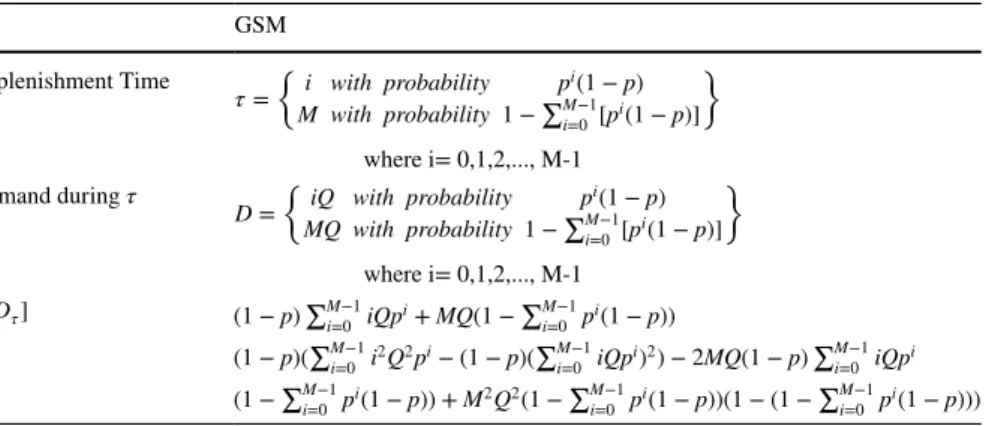
3.1.2 Guaranteed service model
Similar to the SSM, replenishment time definition for the GSM is characterized by the delay. Delay follows a truncated geometric distribution, where M is the maxi-mum delay to satisfy guaranteed service time.
The demand during replenishment time also follows a truncated geometric distri-bution with parameter p. The expressions for the distridistri-bution of the replenishment time, distribution of demand during replenishment time, expected demand and
vari-ance of demand during replenishment time are presented in Table 2.
The DTMC model used is similar to the one in the SSM. The only difference is that, if there are M consecutive periods of no production, outsourcing is performed so that the guarantee given can be realized. For the same state definition as in the SSM (net inventory at the end of a period), a probability transition matrix is
speci-fied and presented in “Appendix 2”. However, in the case of the GSM, the number
of states is finite. As an operational decision, outsourcing is done when there are
M periods of delay (at state (−M + K)Q ), by satisfying only Q backlogs (i.e. the
demand received M periods ago). Then, if production is realized, it produces up to
KQ, otherwise the state will be (−M + K)Q rather than (−1 − M + K)Q . Thus, when
production is not realized for consecutive M periods, demand is outsourced. Steady-state probabilities are,
Performance measures we are interested—expected ending on-hand inventory, expected number of backlogs and expected number of outsourced units- can be writ-ten as (3) E[Backlog] = p ( Q ∞ ∑ i=0 i𝜋−i ) = Qp K+2 1− p 𝜋K −n= pn(1 − p) for n = 0, … , M − 1 𝜋 −M+K= pM
Table 2 Details of the GSM for single-stage model
GSM Replenishment Time 𝜏=� i with probability p i(1 − p) M with probability 1−∑Mi=0−1[pi(1 − p)] � where i= 0,1,2,..., M-1 Demand during 𝜏 D=� iQ with probability p i(1 − p) MQ with probability 1−∑Mi=0−1[pi(1 − p)] � where i= 0,1,2,..., M-1 E[D𝜏] (1 − p)∑M−1 i=0 iQp i+ MQ(1 −∑M−1 i=0 p i(1 − p)) 𝜎2 𝜏 (1 − p)( ∑M−1 i=0 i 2Q2pi− (1 − p)(∑M−1 i=0 iQp i)2) − 2MQ(1 − p)∑M−1 i=0 iQp i (1 −∑Mi=0−1pi(1 − p)) + M2Q2(1 −∑M−1 i=0 p i(1 − p))(1 − (1 −∑M−1 i=0 p i(1 − p)))
Note that we compute the expected outsourced quantity as given in Eq. (6). We believe this quantity is instrumental for comparing models with the GSM regime to models with the SSM regime.
3.1.3 Generalization for non‑zero lead times
Now consider L + 𝜏 where L is an integer denoting the transportation time between stages and 𝜏 is the random variable as defined before. L + 𝜏 stands for the replen-ishment time random variable in the case of non-zero transportation time. Note that when L is different than zero, the order-up-to level will be defined as (K + L)Q for integer L values. Hence, the states will start from (K + L − L)Q = KQ ,
(K + L − L − 1)Q = (K − 1)Q and so on. Therefore, the transition matrix remains
unchanged, and the steady-state probabilities are the same as in the case L = 0 . Then all terms computed for the model remain the same, except that there will be a pipe-line inventory to accommodate L.
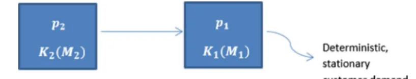
3.2 Two‑stage problem
When the problem has two echelons, Fig. 3 represents the operations. In this setting,
Stage 2 supplies work-in-process inventory to Stage 1, and each stage has its own
no production probability as p2 and p1 , given that raw-material inventory is present.
We make two assumptions:
1. It is assumed that there is an ample supply for Stage 2. The service model for Stage 2 can be the SSM or the GSM.
2. Transportation time for a product to reach Stage 1 (L2) , and transportation time
for a product to reach the customer (L1) are assumed to be zero to ease notation
and exposition.
Figure 2 provides the order of events structure for two-stage system. Stage 2
has an order-up-to level K2Q , and if GSM, M2 denotes the number of
consecu-tive periods with no supply needed to invoke subcontracting. Stage 1 can
oper-ate according to the GSM or the SSM. Let K1 denote the multiplier of Q for the
(4) E[INj] = Q K−1 ∑ i=0 (K − i)𝜋K−i= Q [ K−p(1 − p K) 1− p ] (5) E[Backlog] = Qp (M−K−1 ∑ i=0 i𝜋−i+ (M − K)𝜋−M+K ) (6) E[Outsourced] = Qp𝜋−M+K= QpM+1
order-up-to level and M1 , in the case of the GSM, denote the number of consecu-tive unsuccessful production attempts needed to invoke subcontracting. Stage 1 can keep work-in-process inventory received from Stage 2, as well as finished goods inventory. Note that in case it has received the supply and cannot produce in a period, Stage 1 carries the work-in-process as inventory (in its inbound).
While modeling the two-stage problem, the impact of Stage 2’s operations on Stage 1 should be reflected. To do so, operations of both stages should be tracked and indicated in the transition matrix by characterizing an aggregate state definition for the whole system. (FG2, FG1, RM) is defined as the state of DTMC where FG2 represents Stage 2’s net finished goods inventory at the end of a period, FG1 represents Stage 1’s net finished goods inventory at the end of a period, and RM represents Stage 1’s work-in-process inventory (i.e., raw material supplied by Stage 2) on hand at the end of a period (Note that FG2 and FG1 can be positive or negative whereas RM is always non-negative.).
Given our problem structure, we can mention four different regimes for a two-stage problem: Let the notation X/Y denote the regime followed in a two-two-stage problem, where X is the regime for Stage 2 and Y is the regime for Stage 1; X and Y can be either SSM or GSM. The analysis below is for a GSM/GSM regime when Q = 1 , for simplicity of exposition.
When both stages operate according to the GSM, possible values of the
deci-sion variables are i = 0, 1, 2, … , M2 , j = 0, 1, 2, … , M1 and k = 0, 1, 2, … , M1 .
k ≤ j because raw material accumulates only when Stage 1 cannot produce. If i > K2 then, j ≥ i − K2 as when Stage 2 has negative inventory, it cannot supply
to Stage 1. If i < M2 then k + K1− j > 0 . If i = M2 then M1>k > K1− j > 0 and
other k’s are not possible.
Let the state at the end of period t be (K2− i, K1− j, k) and at the end of period
t+ 1 be (K2− i�, K1− j�, k�) . The following cases can be written:
• Case 1 Both stages can realize production with probability (1 − p2)(1 − p1) ,
then (i�, j�, k�) = (0, 0, 0).
• Case 2 Stage 2 can realize production but Stage 1 cannot realize production
with probability (1 − p2)p1 , then Stage 2 supplies all raw material that Stage 1
needs. If K1− j > 0 , Stage 1 needs one unit of raw material. Otherwise, Stage
1 should accumulate enough raw material inventory to raise the finished goods
inventory up to K1 . In this case, Stage 1 needs K1− FG1 − RM + 1 (FG1 is
finished goods inventory at the end of period t at Stage 1, RM is raw material inventory at the end of period t at Stage 1, +1 indicates the demand of Stage
1 from Stage 2) units. Note that for this example, FG1 = K1− j and RM = k . Then the supplied amount is j − k + 1 . Hence,
1. If K1− j > 0 , (i�, j�, k�) = (0, j + 1, k + 1)
2. If j≠ M1 and K1− j ≤ 0 , (i�, j�, k�) = (0, j + 1, j + 1)
3. If j= M1 and K1− j ≤ 0 , (i�, j�, k�) = (0, j, j)
• Case 3 Stage 2 cannot realize production but Stage 1 can realize production with
probability (1 − p1)p2 , then
1. If i≠ M2 and i < K2 , (i�, j�, k�) = (i + 1, j − k − 1, 0)
2. If i≠ M2 and i ≥ K2 , (i�, j�, k�) = (i + 1, j − k + 1, 0)
3. If i= M2 , (i�, j�, k�) = (M2, j− k, 0)
• Case 4 Both stages cannot realize production with probability p1p2 , then
1. If i≠ M2 and i < K2 , j ≠ M1 ; (i�, j�, k�) = (i + 1, j + 1, k) 2. If i≠ M2 and i ≥ K2 , j ≠ M1 ; (i�, j�, k�) = (i + 1, j + 1, k + 1) 3. If i≠ M2 and i < K2 , j = M1 ; (i�, j�, k�) = (i + 1, M1, k) 4. If i≠ M2 and i ≥ K2 , j = M1 ; (i�, j�, k�) = (i + 1, j, k − 1) 5. If i= M2 , j ≠ M1 ; (i�, j�, k�) = (M2, j+ 1, k + 1) 6. If i= M2 , j = M1 ; (i�, j�, k�) = (M2, M1, k)
Following these possible cases, an example transition matrix when K1= 1, M1= 2
and K2= 1, M2= 2 is given in “Appendix 3”. Among all possible service model and
parameter combinations, this example is the one that has the smallest total number of states (8 states). Thus, obtaining the steady-state probabilities is straightforward. In general, for a GSM-GSM system we expect that an exact solution can be com-puted. However, one can observe that solving problem exactly will suffer from the curse of dimensionality very rapidly as the parameters of the problem get bigger. Furthermore, as the number of states increases and explodes, the accuracy of the computations will be questionable. Note also that for other combinations of service regimes, obtaining an exact solution will either be impossible or require very long computation times.
In the next section, we present an approximation method to obtain the steady-state probabilities.
4 An approximation to compute steady‑state probabilities
4.1 Two‑stage problem
For a problem of realistic size, the number of states will explode, making the computation of the exact solution practically impossible. Hence, we propose an approximation. Decomposition and aggregation methods are applied if a huge
state space makes the numerical solution of Markov Chains too slow or
impossi-ble. Weiss et al. (2019) review possible approaches. Decomposition methods are
promising as they can be implemented for larger systems. The classical approach
of Gershwin (1987) decomposes an N-station line into a set of N − 1 two-station
lines. The buffer capacities in the subsystems are the same as in the original line. However, the station characteristics, such as processing times, inter-failure times and repair times are iteratively modified such that the material flow in the sub-system follows the behavior of the original line, and all two-station lines have the same throughput. Hence, conservation of flow is maintained.
Given the special structure of the environment studied, if both stages are oper-ated according to the SSM, we observe the following:
Observation 1 For the SSM, if Stage 2 does not satisfy the “work-in-process”
demand of Stage 1 (can be in the form of raw material) in a given period due to lack of inventory, the probability that it will satisfy in the next period is always the
same and equal to (1 − p2) . Hence, by following the work-in-process inventory and
finished goods inventory − a state vector with two elements –, for Stage 1, we can exactly represent the desired structure of the system with the transition probabilities
affected by a single term, call it supply probability, 𝜋Sj . Note that 𝜋S2 is the
probabil-ity that Stage 2 is satisfying Stage 1’s demand and can simply be computed as the sum of limiting probabilities of those stages that actually supply. Besides, this prob-ability of having a supply at any state is the same for all inventory levels of Stage 1.
Given Observation 1, we are now ready to implement the approximation pro-cedure for an arbitrary two-stage model, where each stage is operated accord-ing to either the SSM or the GSM. The method is exact if the supplyaccord-ing stage is operated according to the SSM and approximate for the GSM. Nevertheless, we expect the approximation to be quite accurate.
The second stage of the two-stage environment can be modeled as a DTMC. The state definition for Stage 2 will be the same as for a single-stage model. Let
𝜋S2 be defined as the steady-state probability that there will be a supply from
Stage 2. It should be noted that supply is possible when the ending inventory level is above zero or when the stage started with inventory level below (or equal to) zero but production is realized in the period. The first and second terms in
Eqs. (7) and (8) indicate these cases, respectively. The third term in the GSM
reflects satisfying demand via outsourcing. As a result, using the results of the
one-stage problem, 𝜋S2 can be written as
As Stage 1 can keep both finished goods inventory produced and work-in-process inventory received from Stage 2, (i, j) is defined as the state of Stage 1, such that i (7) SSM: 𝜋S2= K2−1 ∑ i=0 𝜋 (K2−i)+ (1 − p1) ∞ ∑ i=K2 𝜋 (K2−i) (8) and GSM: 𝜋S2 = K2−1 ∑ i=0 𝜋 (K2−i)+ (1 − p1) M2−1 ∑ i=K2 𝜋 (K2−i)+ 𝜋(K2−M2)
represents the finished goods inventory and j represents the work-in-process inven-tory at the end of a period. General state transitions can be specified as follows:
If the state is (K1− i, j) at the end of period t and (K1− i
�
, j�) at the end of period
t+ 1:
Case 1 Production is realized and supply is received with probability 𝜋S2(1 − p 1) ,
then (i�
, j�) = (0, 0).
Case 2 Production is realized but supply is not received with probability
(1 − 𝜋S2)(1 − p
1) when j > 0 then (i
�
, j�) = (i − j + 1, 0).
Case 3 Production is not realized but supply is received with probability 𝜋S2p 1
then (i�
, j�) = (i + 1, i + 1).
Case 4 Production is not realized and supply is not received with probability
(1 − 𝜋S2) when j = 0 then (i�, j�) = (i + 1, 0).
Case 5 Production is not realized and supply is not received with probability
(1 − 𝜋S2)p
1 when j > 0 then (i
�
, j�) = (i + 1, j).
As stated in the beginning, there is no capacity restriction, and hence when a stage is successful in production, it consumes all the work-in-process inventory
available and tries to produce up to K1Q units, which is the order-up-to level. Hence,
to reflect this in transition probabilities, the state definition includes the backlogged quantity as well. This can be observed in the transition matrix, given in “Appendix
5” and “7”. Let us now consider the two possibilities of operation in Stage 1:
Stage 1 operates according to the SSM. We follow the order of events as given in
Fig. 2. Stage 1 operates according to the SSM and Stage 2 can be either the SSM or
the GSM, simply represented by the appropriate 𝜋S2 . The expressions for the
distri-bution of the replenishment time, distridistri-bution of demand during the replenishment time, expected demand, and variance of demand during the replenishment time are
presented in “Appendix 4” for the transition matrix in “Appendix 5”.
We follow the same sequence to derive equations. Define 𝜋(i,j) as the steady-state
probability of being in state (i, j), indicating the probability of ending a period with
i units of net finished goods inventory and j units of work-in-process inventory. One
can observe that since the number of states is infinite, some of the steady-state val-ues include infinite sums. However, we observed that all the terms can be written as
a function of 𝜋(K1−1,0) , and approximating infinite sums using truncations, values can
be computed numerically. This truncated state is named as a dummy state and when the steady-state values are found, the dummy state is discarded so that remaining steady-state values can be normalized.
Expected ending on-hand inventory is then computed as
Expected work-in-process (WIP) inventory on-hand is derived as
Expected backlog can be found by
(9) E[INj] = Q K1−1 ∑ i=0 i ∑ j=0 (K1− i)𝜋(K 1−i,j) (10) E[WIP] = Q ∞ ∑ i=0 i ∑ j=0 j𝜋(K 1−i,j)
Last, the supply probability of Stage 1 ( 𝜋S1 ) can be defined by using the results of
the two-stage problem as,
Stage 1 operates according to the GSM. Before we proceed, we first need to set a
detailed outsourcing policy for Stage 1 that considers the WIP issue, similar to the
exact model described in Sect. 3.2. Once production has not been possible for M1
consecutive periods and thus finished goods inventory is zero, Q units of finished goods inventory are subcontracted. In this way, only the order that should have been
sent M1 periods ago is satisfied. Hence, rather than subcontracting the accumulated
backlog during the M1 periods’ delay, we just satisfy the demand for which the
max-imum service delay ( M1 ) has occurred. Then, after outsourcing and satisfying the
demand, if Stage 1 can perform production and the supply is available, it produces
up to K1Q . If it cannot realize production, either due to its process uncertainty or
because supply is not available, its finished goods inventory stays the same in the transition matrix, and one period demand is outsourced. If production is not
real-ized although supply is available, the work-in-process inventory level becomes M1Q
rather than (M1+ 1)Q to avoid keeping unnecessary inventory. This can be regarded
as Stage 1 giving the extra work-in-process inventory back to the supplier, with zero transition cost, and the outsource facility can be regarded as using this work-in-pro-cess inventory to produce one unit of finished good. The expressions for the distri-bution of the replenishment time, distridistri-bution of demand during the replenishment time, expected demand and variance of demand during replenishment time are
pre-sented in “Appendix 6”.
As an illustration, the transition matrix for Stage 1, constructed using these
assump-tions for the GSM, can be found in “Appendix 7” (Q is assumed to be equal to 1,
with-out loss of generality). Steady-state probabilities can be found using this transition
matrix, where 𝜋(i,j) is the probability of being in state (i, j).
Performance measures that interest us (expected ending on-hand inventory, expected WIP inventory on-hand, expected number of backlogs and expected number of out-sourced units for Stage 1) are presented below:
(11) E[Backlog] =Q[(1 − p1) ∞ ∑ i=K1+1 i−K1 ∑ j=0 (i − K1+ 1 − j)𝜋(K1−i,j) + p1 ∞ ∑ i=K1 i ∑ j=0 (i − K1+ 1)𝜋(K 1−i,j)] (12) 𝜋S1= K1−1 ∑ i=0 i ∑ j=0 𝜋 (K1−i,j)+ (1 − p1) ∞ ∑ i=K1 i ∑ j=0 𝜋 (K1−i,j) (13) E[INj] =Q K1−1 ∑ i=0 i ∑ j=0 (K1− i)𝜋(K1−i,j)
Finally, the supply probability of Stage 1 ( 𝜋S1 ) can be defined by using the results of
the two-stage problem as
4.2 Generalization of the approximation to N‑stage problem
Note that we decomposed the two-stage problem by defining the probability of
sup-ply [see Eqs. (7), (8), (12) and (17)]. One should first use Eqs. (7) or (8) for the
most upstream stage to obtain the supply probability according to the single-stage
model. Then for the next downstream echelon, Eqs. (12) or (17) from the two-stage
problem should be used. Once we characterize each stage’s supply probability as 𝜋Sj ,
the problem can be sequentially solved for each stage. The number of stages in the model can be more than two by using the upstream stage’s supply probability which will correspond to its service level and the downstream stage’s state transition prob-abilities which will be shaped according to supply and process probprob-abilities. The states of the downstream stages will be similar to Stage 1 in our model, possibly with a different K value. Hence, the problem can be solved separately for all stages in a serial network. Once the upstream stage’s service level is set, all the other fac-tors will be shaped accordingly. Note that this decomposition enables one to utilize different service models in different stages. A different decomposition method can
be found in de Kok and Visschers (1999).
For the computation of the steady-state probabilities of serial N-stage systems under the decomposition scheme proposed, the algorithm below is implemented. Note that each stage can be operated by either the SSM or the GSM.
(14) E[WIP] =Q M1 ∑ i=0 i ∑ j=0 j𝜋(K 1−i,j) (15) E[Outsourced] =Qp1 M1 ∑ j=0 𝜋 (K1−M1,j) (16) E[Backlog] =Q [ (1 − p1) M1−1 ∑ i=K1+1 i−K1 ∑ j=0 (i − K1+ 1 − j)𝜋(K1−i,j) + p1 M1 ∑ i=K1 i ∑ j=0 (i − K1+ 1)𝜋(K 1−i,j) + p1(M1− K1) M1 ∑ j=0 𝜋 (−M1+K1,j) ] (17) 𝜋S1= K1−1 ∑ i=0 i ∑ j=0 𝜋 (K1−i,j)+ M1 ∑ j=0 𝜋 (K1−M1,j)+ (1 − p1) M1−1 ∑ i=K1 i ∑ j=0 𝜋 (K1−i,j)
Step 1 Solve the N’th stage by using the single-stage problem to compute
steady-state probabilities.
Step 2 Compute 𝜋SN and call it the upstream stage’s supply probability by using
Eqs. (7) or (8).
Step 3 Go to the next downstream stage. By using the upstream stage’s supply
probability, solve the two-echelon problem and obtain steady-state values.
Step 4 Compute 𝜋SN−1 and call it the upstream stage’s supply probability by using
Eqs. (12) or (17).
Step 5 Repeat step 3 by using the supply probability of the upstream stage, for the
computations of the next downstream stage until all stages are covered.
5 Numerical experiments and evaluation of results
In the next subsection, we numerically investigate the quality of the approximation
proposed in Sect. 4. In Sect. 5.2, we present the results of a numerical experiment
we conducted, in which we enumerate all decision variables and compute perfor-mance measures.
5.1 Quality of approximation
The main motivation of the proposed approximation is to avoid the curse of dimensionality. To test the quality of the approximation, we make the following observations.
Observation 2 As K increases the probability of supply is going to increase, and
hence the relative effect of an error in computing will have a tendency to decrease.
Observation 3 As M for the GSM increases, the system looks more like the SSM.
The approximation proposed is exact when the SSM is used; hence, we expect the relative error in the approximation to have a decreasing tendency as M increases.
Observation 4 Following Observation 2 and Observation 3, a two-stage system
where both stages are operated according to the GSM, with smallest possible K and M values, is expected to yield the largest error for the proposed approximation.
Hence, we set K1 = K2= 1 and M1= M2= 2 for our numerical experiments.
Note that we analyze the exact solution described in Sect. 3.2 and the
approxima-tion described in Sect. 4.1. Thus, we compare the exact solution for Stage 1 with the
approximation computed by the algorithm given in Sect. 4.2.
Table 3 presents the results for various p1 , p2 combinations. As can be observed,
the approximation performs quite well. When the probability of no production increases, the gap between the results of the exact solution and the approxima-tion increases. However, even in that case the approximaapproxima-tion is accurate up to two digits. More important, quantities that are likely to be used as parts of any
perfor-mance measure, which are listed in the last four columns of Table 3, indicate that the
5.2 Computational results via enumeration
In Sect. 4.2 we present an algorithm to compute steady-state probabilities for each
stage given K and M values for different stages. We restrict our computations to two-stage systems only. We approach the problem by stating a service level for Stage 1. Note that we enumerate all possible decisions (in this case K’s, and M’s if a stage is GSM) that will yield the desired service level for Stage 1. Here, the
service level the end customer faces corresponds to 𝜋S1 by definition.
Before enumerating all possible solutions, one can compare the quantities of the GSM regime with those of the SSM regime given a fixed supply prob-ability. The following observations are made: As M increases, expected finished goods inventory decreases for the GSM since probabilities for states with less finished goods inventory are larger, whereas expected work-in-process inventory increases. As K increases, finished goods inventory increases for both regimes. However, as K varies, expected work-in-process inventory stays the same for both regimes, as work-in-process is related to supply probability of the upstream stage. The SSM regime keeps less finished goods inventory and more work-in-process
inventory than the GSM regime for the same 𝜋S1 value whereas the supply
prob-ability of GSM is greater than the supply probprob-ability of the corresponding SSM. Finally, the SSM has more expected backlogs than the corresponding GSM.
Table 3 Performance of the approximation
Stage 1 𝜋s Expected subcon-tracted Expected end-ing on-hand inv. Expected WIP
Inv. Expected backlog
p1= 0.05 Exact 0.9975 0.0001 0.9476 0.0525 0.0026 p2= 0.05 Approximation 0.9975 0.0001 0.9478 0.0525 0.0026 p1= 0.1 Exact 0.9902 0.0011 0.8910 0.1099 0.0109 p2= 0.1 Approximation 0.9903 0.0011 0.8920 0.1099 0.0108 p1= 0.1 Exact 0.9908 0.0010 0.8977 0.1100 0.0102 p2= 0.05 Approximation 0.9908 0.0010 0.8979 0.1100 0.0102 p1= 0.1 Exact 0.9878 0.0014 0.8640 0.1096 0.0136 p2= 0.2 Approximation 0.9885 0.0014 0.8716 0.1096 0.0128 p1= 0.2 Exact 0.9629 0.0093 0.7680 0.2384 0.0464 p2= 0.2 Approximation 0.9642 0.0091 0.7755 0.2386 0.0449 p1= 0.05 Exact 0.9958 0.0002 0.9120 0.0524 0.0044 p2= 0.2 Approximation 0.9962 0.0002 0.9197 0.0524 0.0040 p1= 0.05 Exact 0.9972 0.0001 0.9405 0.0525 0.0030 p2= 0.1 Approximation 0.9972 0.0001 0.9415 0.0525 0.0029 p1= 0.2 Exact 0.9667 0.0083 0.7920 0.2396 0.0416 p2= 0.1 Approximation 0.9669 0.0083 0.7931 0.2396 0.0414 p1= 0.2 Exact 0.9677 0.0081 0.7980 0.2399 0.0404 p2= 0.05 Approximation 0.9677 0.0081 0.7982 0.2399 0.0404
In the numerical analyses we consider combinations of various SSM and GSM systems for both stages and compute the expected total cost of inventories, and effects on the expected outsourcing quantities.
Expected total ending on-hand inventory cost is found according to either Eqs. (9)
or (13) for Stage 1 and according to either Eqs. (2) or (4) for Stage 2. We set inventory
holding cost as 1 for Stage 1 and 0.5 for Stage 2. Hence, expected ending on-hand inventory cost is found by multiplying holding costs by ending on-hand inventory amounts. For Stage 1, expected work-in-process inventory is again found according
to Eqs. (10) or (14) and is included in the expected total ending on-hand inventory
cost. Expected backlog quantities are calculated according to Eqs. (11) or (16).
The values considered for numerical examples are as follows: For any stage and any regime K = 1, 2 , and for the GSM regime at any stage
M= K, K + 1, K + 2, K + 3 . In total 100 combinations of these 10 different cases
are evaluated when the probability of no production is taken as 0.2 for all cases.
5.2.1 Expected total carrying cost
For ease of presentation, we clustered the comparison cases according to the service level achieved by Stage 1. The service level ranges from 95.3% to 96.8% and from
99% to 100% . Therefore, we clustered the cases according to the minimum service
level obtained ( 95.3% and 99% ). Detailed results for the best 10 combinations based
on “expected total ending on-hand inventory costs” are presented in Tables 6 and 7 in
“Appendix 8”, following other work in the area that presents only these costs (Graves
and Willems 2003). As expected, SSM regime yields lower expected on-hand
inven-tory cost values when the service level is not high. When it is high, we expect the GSM to be relatively effective.
Service level is [95.3 %, 96.8%] Table 6 in “Appendix 8” ranks the models when the service level of the system is around 95.3 %. When both stages are operated
under the SSM and K1= K2 = 1 , the system has the minimum expected total ending
on-hand inventory cost. It can be observed that the GSM when K2 = 1 for Stage 2
performs better than other combinations. The best combination for the GSM is when
K2 = 1 and M2= 4 (the limit we tried, and hence closest to the SSM regime).
Service level is [99 %, 100%] Table 7 in “Appendix 8” ranks the cases in increasing order of the total expected ending on-hand inventory cost where the ser-vice level of the system is around 99 %. The best case is an SSM/GSM combination
when K2= 1 and K1= 1, M1= 1 . The explanation is straightforward: As the SSM
keeps more stock for the required service level, a combination that uses the GSM regime outperforms an SSM/SSM system.
5.2.2 Measuring effects of outsourcing
One of the assumptions made by Graves and Willems (2003) for the GSM regime,
is that the excess demand over the accepted maximum bound is outsourced from another source to satisfy customer requirements. However, there is no additional term that represents the outsourced amount in the objective function, assuming that
the expected subcontracting cost will be negligible. Note that we followed the same assumption in our work. Here we analyze the effect of that assumption.
For the analysis, we consider two systems where one system uses the GSM regime only (call it the GSM/GSM system) and the other one uses the SSM regime (call it the SSM/SSM system). Note that in order to make a reasonable comparison, the expected ending on-hand inventory cost of the SSM/SSM system should be larger than that of the GSM/GSM system, while both should yield approximately the same service level. Given these conditions, our aim is to find a threshold outsourcing cost per unit for Stage 1 (the outsourcing cost for Stage 2 has the same proportion as
hold-ing costs, i.e., = h2∕h1 ), which will yield the same expected costs for both systems.
To come up with a comparison, we consider minimum service level clusters
95.3% and 99%, and the SSM/SSM system with K2= 2 , K1= 1 and K2= 2 , K1 = 2 ,
respectively. Those are the cases that yield a higher expected on-hand inventory cost compared to some GSM/GSM combinations. We take the difference of expected ending on-hand inventory costs and divide the difference by the cost of total net expected outsourced in the GSM/GSM system (expected outsourced in Stage 1 +
(h2∕h1) * expected outsourced in Stage 2) to find the threshold outsourcing cost that
will equate the expected total cost of the two cases considered. Using the threshold cost found, we compute the expected cost of subcontracting as a percentage of total expected cost of ending on-hand inventory, and we represent the threshold cost as a percentage of the expected backlog cost implied by the service level used for the
stage. The results are shown in Tables 4 and 5.
Table 4 Analyses with threshold outsourcing costs when service level is at least 95.3% (range: [95.3% ,
96.8%]) Case number
K2 M2 K1 M1 Total expected subcontracting cost at threshold as a percentage of total expected ending on-hand inventory holding cost (%)
Total expected subcontract-ing cost at threshold as a percentage of unit total expected backlog cost (%)
1 1 4 2 4 15 28
2 1 4 2 5 7 6
3 1 3 2 4 7 13
Base case 2 NA 2 NA – –
Table 5 Analyses with threshold outsourcing costs when service level is at least 99% (range: [99% ,
100%])
Case number K2 M2 K1 M1 Total expected
subcontract-ing cost at threshold as a percentage of total expected ending on-hand inventory holding cost (%)
Total expected subcon-tracting cost at threshold as a percentage of unit total expected backlog cost (%)
1 1 2 1 2 23 26
2 1 3 1 2 30 35
3 1 4 1 2 32 38
Both results indicate that it is beneficial to take into account the effect of out-sourced quantity in certain cases, as opposed to not considering it at all. Especially when higher service levels are considered, subcontracting is beneficial with a rela-tively low threshold value, which implies that the GSM regime is likely to be a more expensive choice.
6 Conclusions and future work
For the single-stage system, we can evaluate steady-state probabilities of a DTMC exactly when service regime parameters are (K for the SSM and K and M for the GSM) supplied. The two-stage system can also be represented exactly by a DTMC, when each stage is allowed to follow either the SSM or the GSM regime. However, when it comes to evaluating steady-state probabilities, the number of states grow exponentially prohibiting sound computations. Nevertheless, we formulate a GSM/ GSM operated two-stage system and compute the steady-state probabilities exactly. Once we have steady-state probabilities, we can obtain quantities for expected end-ing on-hand inventory of finished goods and work-in-process inventories, as well as expected backlogs and expected outsourced amount.
For more realistic serial systems, we offer an approximation. We decompose the stages by defining the probability of supply from one stage to the next. We numeri-cally show that the decomposition approximation is fairly accurate for the two-stage model.
To analyze the systems further, we use total enumeration considering all combi-nations (GSM, SSM for any stage) of service regimes with varying K and M values. We cluster combinations that yield reasonably close service levels and compare dif-ferent systems. Results suggest that for reasonable service levels, an SSM/SSM sys-tem results in the lowest total expected on-hand inventory costs. However, when the service level is relatively higher, we expect the GSM to be relatively effective.
Finally, we make some computations to test the assumption made in the litera-ture that expected subcontracting cost is negligible. We conclude by showing that expected quantity to outsource may well be an important consideration, and hence should not be ignored.
One immediate extension of the current work is to model a two echelon assem-bly system. As all suppliers operate according to a base stock policy and a service model (SSM or GSM), the probability of supply for each supplier can be obtained by solving the single-stage problem, as in the two-stage serial system. Therefore, the system can be modeled by using a DTMC structure and probability values can be used in the transitions to reflect a supplier’s effect on Stage 1. The difference between a serial system and an assembly system is in the state representation of Stage 1: Each supplier’s work-in-process inventory in stock should be represented. The size of the state space grows rapidly in this case, and hence solving this prob-lem even computationally may require a different method. Decomposing the model
[see de Kok and Visschers (1999)] appears to be an acceptable direction to proceed,
Future work can also consider the partial supply (production) availability case. Most features of the model may remain the same, except the reflection of the supply uncertainty structure. In the current context, supply uncertainty that the downstream stage faces is a result of production uncertainty at the upstream stage. Hence, sup-ply unavailability can be used to reflect production unavailability. In the extension, desired production quantity may be fully supplied, partially supplied or not
sup-plied at all. Following the structure of Güllü et al. (1999) a DTMC can be specified
requiring an extension to the already existing states.
Appendix 1: Probability transition matrix for single‑stage problem under the SSM K K− 1 K − 2 ... K− n K − n − 1 ... K 1 − p p 0 ... 0 0 ... K− 1 1 − p 0 p ... 0 0 ... K− 2 1 − p 0 0 ... 0 0 ... . . . . K− n 1 − p 0 0 . 0 p ... K− n − 1 1 − p 0 0 . 0 0 ... . . . .
Appendix 2: Probability transition matrix for single‑stage problem under the GSM K K− 1 K − 2 K − 3 ... −M + K + 1 −M + K K 1 − p p 0 0 ... 0 0 K− 1 1 − p 0 p 0 ... 0 0 K− 2 1 − p 0 0 p ... 0 0 . . . . −M + K + 1 1 − p 0 0 0 ... 0 p −M + K 1 − p 0 0 0 ... 0 p
Appendix 3: Probability transition matrix for two‑stage problem under the GSM (1, 1, 0) (1, 0, 1) (1, −1, 2) (0, 0, 1) (0, 1, 0) (0, −1, 2) (−1, 0, 0) (−1, −1, 1) (1, 1, 0) (1 − p1)(1 − p2) (1 − p2)p1 0 p1p2 (1 − p1)p2 0 0 0 (1, 0, 1) (1 − p1)(1 − p2) 0 (1 − p2)p1 0 (1 − p1)p2 p1p2 0 0 (1, −1, 2) (1 − p1)(1 − p2) 0 (1 − p2)p1 0 (1 − p1)p2 p1p2 0 0 (0, 0, 1) (1 − p1)(1 − p2) 0 (1 − p2)p1 0 0 0 (1 − p1)p2 p1p2 (0, 1, 0) (1 − p1)(1 − p2) (1 − p2)p1 0 0 0 0 p2 0 (0, −1, 2) (1 − p1)(1 − p2) 0 (1 − p2)p1 0 0 0 (1 − p1)p2 p1p2 (−1, 0, 0) (1 − p1)(1 − p2) 0 (1 − p2)p1 0 0 0 (1 − p1)p2 p1p2 (−1, −1, 1) (1 − p1)(1 − p2) 0 (1 − p2)p1 0 0 0 (1 − p1)p2 p1p2
Appendix 4: Two‑stage model: expressions for stage 1 for the SSM
SSM Replenishment Time ( 𝜏) 𝜏= � i with probability 𝜋S2(1 − p 1)( ∑i j=0[(1 − 𝜋 S2)i−jpj 1]) � where i= 0,1,2,3,...
Demand during 𝜏 D=�iQ with probability 𝜋S2(1 − p
1)( ∑i j=0[(1 − 𝜋 S2)i−jpj 1]) � where i= 0,1,2,3,... E[D𝜏] Q𝜋S2(1 − p 1)( ∑∞ i=1 ∑i j=0[i(1 − 𝜋 S2)i−jpj 1]) 𝜎2 𝜏 Q 2𝜋S2(1 − p 1)( ∑∞ i=1 ∑i j=0[i 2(1 − 𝜋S2)i−jpj 1]) −[Q𝜋S2(1 − p 1)( ∑∞ i=1 ∑i j=0[i(1 − 𝜋 S2)i−jpj 1])] 2
A pp endix 5: Tw o‑stage mo del: pr obabilit y tr ansition ma trix f or stage 1 under the SSM (K 1 ,0) (K 1 − 1, 0) (K 1 − 1, 1) (K 1 − 2, 0) (K 1 − 2, 1) (K 1 − 2, 2) (K 1 − 3, 0) (K 1 − 3, 1) (K 1 − 3, 2) (K 1 − 3, 3) .. . (K 1 ,0) π S2 (1 − p1 )1 − π S2 π S2 p1 00 0 0 00 0 .. . (K 1 − 1, 0) π S2 (1 − p1 ) 0 0 1 − π S2 0 π S2 p1 0 00 0 .. . (K 1 − 1, 1) π S2 (1 − p1 )( 1 − π S2 )( 1 − p1 )0 0( 1 − π S2 )p1 π S2 p1 00 0 0 .. . (K 1 − 2, 0) π S2 (1 − p1 )0 00 00 (1 − π S2 ) 0 0 π S2 p1 .. . (K 1 − 2, 1) π S2 (1 − p1 )0 0( 1 − π S2 )( 1 − p1 )0 00 (1 − π S2 )p1 0 π S2 p1 .. . (K 1 − 2, 2) π S2 (1 − p1 )( 1 − π S2 )( 1 − p1 ) 00 00 00 (1 − π S2 )( p1 ) π S2 p1 .. . . . . . . . . . . . . . . . . . . . . . . . . . . . . . . . . . . . . . . . . . . .


![Table 5 Analyses with threshold outsourcing costs when service level is at least 99% (range: [99% , 100 %])](https://thumb-eu.123doks.com/thumbv2/9libnet/6005762.126460/21.659.74.588.746.909/table-analyses-threshold-outsourcing-costs-service-level-range.webp)
![Table 7 Service level is at least 99% (range: [99%, 100%]) Total expected ending](https://thumb-eu.123doks.com/thumbv2/9libnet/6005762.126460/28.659.78.587.471.702/table-service-level-range-total-expected-ending.webp)
