Parameter optimized controller design based on frequency domain identification

р ш іш т w iM ïiû j

l-idas

PARAMETER OPTIMIZED CONTROLLER DESIGN

BASED ON FREQUENCY DOMAIN

IDENTIFICATION

A THESIS

SUBMITTED TO THE DEPARTMENT OF ELECTRICAL AND ELECTRONICS ENGINEERING

AND THE INSTITUTE OF ENGINEERING AND SCIENCES OF BILKENT UNIVERSITY

IN PARTIAL FULFILLMENT OF THE REQUIREMENTS FOR THE DEGREE OF

MASTER OF SCIENCE

By

Hakan Koroglu

September 1995

TJ

■ k ó 9 - -1335

I certity that I have read this thesis and that in rny opinion it is fully adequate,

in scope and in quality, as a thesis for the degree of Master of Science.

Assoc. Prof. Dr. Omer McJrgii^Supervisor)

I certify that I have read this thesis and that in my opinion it is fully adequate,

in scope and in quality, as a thesis for the degree of Master of Science.

Prof. Dr. Erol Sezer

I certify that I have read this thesis and that in rny opinion it is fully adequate,

in scope and in quality, as a thesis for the degree of Master of Science.

Assist. Prof. Dr. Orhan Arikan

Approved for the Institute of Engineering and Sciences:

’ rof. Dr. Mehmet BLaray

ABSTRACT

PARAM ETER OPTIMIZED CONTROLLER DESIGN

BASED ON FREQUENCY DOMAIN IDENTIFICATION

Hakan Köroğlu

M.S. in Electrical and Electronics Engineering

Supervisor: Assoc. Prof. Dr. Ömer Morgiil

September 1995

Recently, there has been a great tendency towards the development of itera­ tive design methodologies combining identification with control in a mutually supportive fashion. In this thesis, we develop such an algorithm utilizing non- parametric frequency domain identification methods in order to realize the online iterative design of parameter optimized controllers for a system of un­ known dynamics. The control design is based on the minimization of LQG (Linear Quadratic Gaussian) cost criterion with a two-degree of freedom con­ trol system. This is achieved by the approximation of an optimality relation, which is derived for a particular parametrization of one of the controllers, us­ ing the frequency domain transfer function estimates and application of this together with a numerical optimization algorithm. It is shown that, if the first controller is a FIR filter of length greater than or equal to two times the num­ ber of frequencies present in the reference input, the designed control system is optimal independent of the stabilizing second controller.

Keywords : System identification, adaptive control, parameter optimized con­ trollers, LQG (Linear Quadratic Gaussian) cost.

ÖZET

FREKANS KÜMESİ TANIMLAMASI YOLUYLA EN İYİ

PARAMETRELİ KONTROL SİSTEMİ TASARIMI

Hakan Köroğlıı

Elektrik ve Elektronik Mühendisliği Bölümü Yüksek Lisans

Tez Yöneticisi: Doç. Dr. Ömer Morgül

Eylül 1995

Son zamanlarda, tanımlama ve kontrol etme işlemlerini birbirlerini destek­ leyici mahiyette biraraya getiren ardışık tasarım metodolojilerinin geliştirilmesi yönünde büyük bir eğilim oluşmuştur. Bu tezde, tanınmayan sistemler için, en iyi parametreli kontrol sistemlerinin, ardışık olarak ve çalışma esnasında tasarımı amacıyla, parametreye dayalı olmayan frekans kümesi tanımlama yöntemleri kullanılarak böyle bir algoritma geliştirilmiştir. Kontrol tasarımı, iki kontrol edicili bir kontrol sistemi ile DKG (Doğrusal Kuadratik Gausiyen) bedel kriterinin en düşük değerinin elde edilmesini hedeflemektedir. Bu da, birinci kontrol edicinin belli bir tarzdaki parametre bağımlılığı için elde edilen bir optimalité bağıtısının, frekans kümesi transfer fonksiyonu tahminleri kul­ lanılarak sağlanması ve bunun bir sayısal optimizasyon algoritmasıyla beraber uygulanması yoluyla gerçekleştirilmiştir. Ayrıca, birinci kontrol edicinin, refer­ ans sinyalindeki frekans sayısının iki katı kadar ya da daha fazla uzunlukta bir SDC (sonlu dürtü cevaplı) süzgeç olması durumunda, kararlı olarak tasar­ lanan kontrol sisteminin ikinci kontrol ediciden bağımsız olarak optimal olduğu gösterilmiştir.

Anahtar Kelimeler : Sistem tanımlaması, uyarlamalı kontrol, en iyi parame­ treli kontrol ediciler, DKG (Doğrusal Kuadratik Gausiyen) bedel kriteri.

ACKNOWLEDGEMENT

I would like to express my deep gratitude to my supervisor Assoc. Prof.

Dr. Omer Morgril for his guidance, suggestions and invaluable encouragement throughout the development of this thesis.

I would also like to thank to Prof. Dr. Erol Sezer and Asst. Prof. Dr. Orhan Arikan for reading and commenting on the thesis.

TABLE OF CONTENTS

1 IN TR O D U C TIO N 2

2 N O N PAR AM ETR IC FREQUENCY D O M AIN IDENTIFI­

CATION 5

2. 1 Linear Time Invariant Systems : Some Terminology and Notation 6

2.2 Fourier A nalysis... 8 2.2.1 Periodograms of Finite Duration S ig n a ls ... 9

2.2.2 The Empirical Transfer Function Estimate (ETFE) . . . 10

2.2.3 Smoothing the E T F E ... 14

2.3 Spectral A n a ly s is ... L5

2.3.1 Spectral R ep resen tation ... 16

2.3.2 Transformation of Spectra by Linear Systems 16

2.3.3 The Use of Power Spectrum Estimates in Transfer Func­

tion E stim a tion ... 17

2.4 Improvement of the ETFE Based on the Estimates Obtained

from Different Data S e t s ... 18

3 PAR AM ETER OPTIM IZED LINEAR Q U AD R ATIC GAUS­

SIAN CONTROL 19

3.1 Parameter Optimized Controller D esign... 20 3.2 LQG Optimal C o n t r o l ... 21

3.3 Parameter Optimized Control Based on LQG Performance Cri­

terion 22

3.4 Tracking the Reference Signals of Finite Frequency Content . . . 28

4 ONLINE DESIGN OF IDENTIFICATION A N D CONTROL 31

4.1 Iterative Design of Identification and C on trol... 32

4.2 Alternative A lgorith m s... 35

5 SIMULATIONS 37

6 CONCLUSION 49

LIST OF FIGURES

3.1 LQG Control System... 23

5.1 Tracking of a single frequency sinusoid : A = 0 , ni = 2 , n2 = 2 . 39 5.2 Tracking of a single frequency sinusoid ; A = 0.4 , ni = 2 , «2 = 2 . 39 5.3 Tracking of a single frequency sinusoid : A = 0 , n i = l , n2 = l . 40 5.4 Tracking of a single frequency sinusoid : A = 0.4, ni = 1, U2 = 1. 40 5.5 Tracking of a square wave : A = 0 , ni = 30, U2 = 2 ...41

5.6 Tracking of a square wave : A = 0.4 , ni = 30, n2 = 2... 41

5.7 Tracking of a square wave : A = 0, ni = 2 0, ri2 = 2... 42

5.8 Tracking of a square wave : A = 0.4 , ni = 2 0, n2 = 2... 42

5.9 Tracking of a sawtooth wave : A = 0 , ni = 50, «2 = 1 ... 43

5.10 Tracking of a sawtooth wave : A = 0.4, ni = 50, ri2 = 1 ... 43

5.11 Tracking of a sawtooth wave : A = 0 , ni = 30, «2 = 2 ... 44

5.12 Tracking of a sawtooth wave : A = 0.4 , ni = 30, U2 = 2 ... 44 5.13 Tracking of a multifrequency sinusoid : A = 0, rti = 10, n2 = 1. 45

5.14 Tracking of a riiultifrequency sinusoid : A = 0.4, rq = 10, «2 = 1 . 45 5.15 Tracking of a multifrequency sinusoid : A = 0 , ni = 5 , n2 = 2 . 46 5.16 Tracking of a raultifrequency sinusoid : A = 0.4 , ni = 5 , n2 = 2 . 46

5.17 Tracking of a modulated signal : A = 0, ni = 40, n2 = 1. 47

5.18 Tracking of a modulated signal : A = 0.4, ni = 40, n2 = 1. 47

5.19 Tracking of a modulated signal : A = 0, ni = .35 , U2 = 2. 48

Chapter 1

INTRODUCTION

Many control design techniques rest on the availability of the model of the plant to be controlled. If the model is not present, a model is estimated through the processing of input/output data, and the controller design is based on this estimate. Adaptive control is the area in which the model based design of feedback controllers is combined with the on-line estimation of process models based on input/output data measurements.

Though there is not a generally accepted definition of the terms ‘ adaptive’ and ‘ self tuning’, adaptive control systems are distinguished by their ability to adjust their behaviour to the changing properties of the controlled processes and their signals [16]. There are various types of adaptive control systems (see [15] and [16] for different classifications), however each possess an adap­ tation mechanism which adjusts the controller according to a certain rule. If the adaptation mechanism includes the identification of the process using in­ put/output data and the determination of the controller parameters is based on this identified model, then the system is a model identification based adap­ tive system which is also referred to as a self tuning or a self optimizing system [16]. These terms also describe the automatic adjustment of the controllers when the process has stationary behaviour.

Adaptive controllers with model identification can be designed using para­ metric or nonparametric models. It is important that the model describes the system well enough such that the performance of the designed controller is not much different than that would be obtained with the e.xact system description. This brings into picture the effect of the identified model upon the controller and hence on the closed loop performance of the system. Similarly, the closed loop control action will affect the estimation of the model of the plant. This interplay between the identification and control design is the focal point of [6] and it is analyzed in the context of least squares identification and Linear Quadratic Gaussian Optimal Control.

It is argued in [28] that identification and control design have to be treated as a joint problem rather than two individual problems. Solution of this joint problem during online operation is to be realized using an iterative scheme. Moreover the collection of the data from the closed loop is indicated to be useful for control relevant identification in various studies (see e.g. [.33], [2], [29], [5], [13], [14]). In fact the concept of optimal identification for control originated from [11]. The need for the use of a performance enhancement data filter operating on the identifier signals was advocated in [6]. The dual idea of incorporating the model error information into the control design criterion was proposed in [33]. For further information on the joint design of identification and control, refer to [10] which is a survey paper. As the most recent related sudies, see [9], [13], [14], [34]. Besides these, [14] is an interesting work , pre­ senting an indirect iterative scheme, which estimates the controller parameters directly without the intermediate model identification step.

The iterative scheme developed by these studies aims at designing the iden­ tification and control in a supportive fashion. The use of a nonparametric model for the plant therefore seems to be more rational. The nonparametric methods are adventageous also because they require no assumptions for the model structure, order, etc., of the system.

Hence in our study, we will develop a similar iterative design algorithm utilizing the frequency domain transfer function representation of the system. VVe will study the controller design based on the minimization of the linear quadratic cost criterion. Then we will try to present a general algorithm for the design of an optimum control system. The outline of the thesis will be as

follows. In the next chapter, we will analyze the nonparametric identification in the frequency domain. Estimation of the transfer function of the system based on certain signal processing techniques will be presented. Various methods for the improvement of the estimate will also be discussed. In Chapter 3, we will study the design of parameter optimized controllers. We will fust summarize the linear quadratic gaussian optimal control. Then we will present the design method for the minimization of the linear quadratic gaussian cost criterion with certain types of controllers. Results will be presented for special cases. In Chapter 4, we will propose an iterative design algorithm and discuss various alternatives. Chapter 5 contains some simulation examples in which the iterative algorithm is put into practice. The final chapter gives the conclusions of the thesis and discussions about the future work that can be done.

Chapter 2

NONPARAMETRIC

FREQUENCY DOMAIN

IDENTIFICATION

Identification is the experimental determination of the dynamical behaviour of processes and their signals [16]. This is to be done in order to estimate the future behaviour of the system, or in order to design a controller such that the system behaves in a desired manner.

System identification is based on a representation of the system. For differ­ ent representations there may be different identification techniques. However in each case, the representation (whose structure is predetermined) will be found (or guessed) through the processing of input/output data. If the identifica­ tion type aims at determining the best value of a finite dimensional parameter vector representing the system, then it is called a parametric identification method. The methods in which there is no preselection of a confined set of possible models are called nonparametric methods.

In this chapter we will analyze the nonparametric identification methods for linear time invariant systems, which are based on frequency domain analysis. The study will basically deal with the determination of the transfer function of the system. Then certain ways for the improvement of the estimate will be pre­ sented. A relation will also be formed with spectral analysis. The development given will be applicable during online operation.

2.1

Linear Time Invariant Systems : Some

Terminology and Notation

A system is said to be linear if the response of it to a linear combination of certain inputs is equal to the same linear combination of the responses to the individual inputs [21]. It is said to be time invariant if a time shift applied to the input results in a corresponding time shift of the output [35]. Moreover a system is a causal system if the output at any time depends only on the present and past values of the input.

In this work, we will confine ourselves to linear time-invariant (LTI) discrete-time causal systems. We can denote such systems by

y{t) = P{q)u{t) + v{t) (2.1)

where t is the discrete time index, ic is the input sequence, y is the output

sequence and v is an unmeasured disturbance acting on the output. With q

denoting the forward shift operator (i.e. qu{t) = u{t -f 1)), P{q) is a strictly

proper rational transfer function of q representing the system, as given below.

P {i) = Y

b\q ^ + · · · + bn^q— T in

Thus Eqri. 2.1 describes the discrete input-output relation of the system which is of the form

y{t) + aij/(t — 1) H--- — Ud) — bxu{t — 1) H--- h b„^u(t — n„) -f u ( i ) . Because of the linearity and time-invariance, we can also express the output of an LTI system as a weighted sum of the responses to shifted unit impulses. That is

!/(*) = S - t) + v(t) , (2.2)

where p{r) is the impulse response sequence of the system. This is called

the convolution sum [35]. For causal systems, p(r) = 0, Vr < 0, hence the

summation starts from r = 0.

If we replace q with 2 in the transfer function, we obtain the z-transform of the impulse response of the system.

i ’ (2) = £ p(f)^ ‘ (2.3)

t = —oo

If the impulse response sequence is absolutely summable, the system is said to be BIBO stable (this means that a bounded input will result in a bounded output). With causality which causes the summation to start from r = 0, this

assures that the summation in Eqn. 2.3 is convergent for all \z\ > ₁. Then

P {z) is analytic on and outside the unit circle, which means it has no poles outside the unit circle.

There are other ways of representing linear systems as well. State space models and the difference equations also determine the behaviour of a linear system completely. However our development in this work is not related with these representations. For a thorough analysis of all types of models of LTI systems, see [21, 30]. And for further analysis on LTI systems , refer to [24, 23, 35].

2.2

Fourier Analysis

Sinusoidal sequences are extremely valuable in the analysis of LTI systems. If the system is stable , a sinusoid of frequency u) will result in a sinusoid of the same frequency, but with a change in magnitude and phase, at steady state in

case of no disturbance. The complex number P(e^“ ) (which is P{z) evaluated

at z = e^‘^) determines the change in magnitude and phase therefore giving full information about the steady state behaviour of the system. Thus the function

0 < cu < 2TT, represents the system without disturbance completely at steady state and is called the transfer function (or frequency function) of the system [21]. Thus we can write

where Y {lo) = P i e ^ U i u ) + V{lo) , (2.4) oo t = - o o (2.5) oo t = —oo (2.6) oo v(ui) = E « (O c ·" " ' ■ i = —OO (2.7) oo P { e n = X ; p(i)e-^“ ' , i= —OO (2.8)

are the discrete-time fourier transforms (D T F T ) of the input, output and

disturbance sequences respectively [23]. The DTFTs exist for absolutely

surnrnable sequences. If P{z) has no poles outside the unit circle, P{e^'^) will

converge and it will be P{z) evaluated at z — e^'^. The time domain signals

2.2.1

Periodograms of Finite Duration Signals

The above representation of LTI systems includes infinite duration signals. In practice, all signals will somehow be of finite duration. In that case there is an appropriate representation of signals known as discrete Fourier transform (D F T ).

Consider a finite duration sequence u{t) ■, t = —1. Let Uk be

defined as

2tt

cufc = — k = 0 , l , . . . , N - 1 . (2.9)

Then the DFT sequence is defined as, ([35])

N - l

UN{k) = u(i)e"^‘^*‘ ; A; = 0,1, . . . , - 1.

t= 0

(2.10)

Given the DFT sequence, it is easy to find that, ([21])

(0 = 4 E i = 0,1, . . . , iV - 1.

A;= 0

U

(

.

)

Comparing the DFT of u with its DTFT, it is immediately observed that DFT

is the sequence of equally spaced (a separation of ^ ) samples of DTFT, that is

UN{k) = U{u:)l=^,·, A: = 0,1, . . , A ^ -1.

The value \UN{k)\'^ is therefore a measure of the energy contribution of fre­

2.2.2

The

Empirical Transfer

Function

Estimate

(ETFE)

In a linear system, different frequencies pass through the system independently of each other. The frequency function determines the output behaviour at each frequency. Motivated by Eqn. 2.4, an estimate of the transfer function of the system can be made, based on the processing of input and output sequences.

When the input and output are not of finite duration (or if they are ex­

tremely long), we have to observe them on an interval of length N and use

these observations in the estimation procedure. At this point we have to state a theorem showing the relation between the input and output DFTs when the observation is done in an interval of length N.

T h e o r e m 2.1 : Let P be a LTI, causal and stable system which is represented by Eqn. 2.1. With Uj!j{k) , Y^{k) and V^{k) denoting the N-point DFT se­ quences of u(t), y{t) and v{t) ending with time index n (i.e. DFTs of the signals observed between n — N + I and n), we have

YS{k) = P(e>">)UÍ,{k) + EÍ,{k).^V;l(ky, k = 0 , l , . . . , N - 1 .

2

12

oo

= t = 0, l , . . . , i v - l . (2.13)

T = 1

Proof : This theorem is the same as Theorem 1 of [18] except that here the disturbance acting on the system is also taken into account. We will present the same proof with some simple modifications coming from the addition of the disturbance term.

The frequency domain representation of the system behaviour is given by Eqn. 2.4. From the definitions we have

n-/V CO

UJl,{k) = U{0Jk) - E - E ,

t=z — oo

n - N

Yjl}(k) = Y(co,) - E 2/(<)e-jwkt

_E

t = —oo

From Eqri. 2.4 we have n-N

Yj^ih)

On the other hand from Eqn. 2.2 and with the fact that p(r) is zero for r < 0

as the system is causal, we find

n —N n —N 00 t = —oo t= — 00 T =0

=

p(r)e-^‘^‘=^

n(< -

+

E «(Oe - E i/(0e

= E P(r)e-^""‘^( E

- E

- E

E

E

.

(Note that for r = 0, the term in paranthesis becomes zero, so summation starts from r = 1.)

Similarly we can find

00 00 ¿ = 71+1 00 ¿ = 71+1

= - E

p

(^K'^ E

- E

Inserting these in the equation for Y'^^{k), we end up with Eqn. 2.11 where г -Л /

5^ u{t)e - J2 w(0e ,

i = n —/V —r - f l ¿=n —r+1

r = l

which can be shown to be equivalent to Eqn. 2.12. □

Here E'^(k) comes into picture due to the use of finite length data. Thus

increasing N reduces its magnitude. Moreover a bound can be found on its

magnitude in case of certain assumptions. This is examined in the following theorem.

T h e o r e m 2.2 : Let the input be bounded as |u(i)| < U, Vi. Under the asumptions of Theorem 2.1, the magnitude of E^{k) is bounded for each k. Moreover if the input is periodic with period To and if N is an integer multiple of To, then E^{k) = 0, Ук.

P r o o f : This theorem is closely related with Theorem 2 of [18]. We will

present a similar proof. First we should remember from the proof of the pre­ vious theorem that

oo n —N n

£n( 4 = E E •‘(t)e ·'“ * ' - E “ (О с -'" “ ) .

r = l ¿ = 71 —Л/ —r -f l ¿ = 7 l-r + l

Then using the triangle inequality we get

OO n —N n

|E

k

(*)I<EW^)II E

E

Note that, since the system is (exponentially) stable, p(r) decays exponentially, hence the surtirnation given above remains finite.

If the input is periodic with period To = ^ where a iponentially, hence the summation given above remains finite.

If the input is periodic with period To = -^ where a is an integer, then it will also be periodic with period N. We will then have

n - N

t = n —N —r ^ \

u{t -¿ = n —T -fl

t=n—T-f-1

Inserting this result in the expression for E^{k), we see that the error becomes

zero for all k. □

Motivated by the two theorems above, we can introduce the following esti­ mate for the transfer function of the system.

p n ^ . jL _ f| I A/· — 1 _(2.14)

This estimate is called the empirical transfer function estimate (ETFE), [21].

Note that we must have U'^{k) ^ 0, otherwise the ETFE is simply undefined.

The estimation error is then

= P A: = 0,1, . . . , iV - 1. (2.15)

For our estimate at the frequency wjt to be reasonable, it is obvious that we

must use a high enough N such that E^{k) is small. Moreover the disturbance

power at that frequency must be small when compared with the input power.

Once the ETFE is determined at certain points (at a group of u>k for

k G C {0,1,. . , W — 1}), the value of the transfer function at other

frequencies can be estimated through interpolation. In fact the transfer func­ tion can then be found through curve fitting based on these finite number of

data. Of course these procedures will be applicable for the case where P{e^^)

is a smooth function of w (i.e. its magnitude and phase), and this is already the case when P{q) is a rational polynomial.

2.2.3

Smoothing the ETFE

Smoothness means that there is some correlation between the values of the transfer function at the neighbouring frequencies. That is the value of the transfer function at a frequency o;o is related to the values of it at a;o — and

uiQ + 6, and the relation decreases as S becomes larger. If this is the case, then the value of the transfer function at o;o can be estimated as a linear combination of the estimates at the neighbouring frequencies, in which the larger effect of the nearer frequencies is taken into account. Moreover it is also important to decrease the effect of the estimates whose deviations from the true values are

large. In other words, if is large, then the weight of in the

combination should be small. From Eqn. 2.15 we see that the estimation error at a certain frequency is large if the ratio of the input power to the disturbance power at that frequency is small. Thus if the disturbance power is a slowly varying function of w, then the ETFE can be improved as

P i(e « ) =

where

O'TT

ak = W{k - ko) I U^^{k) p; = 0 , 1 , . . . , yV - 1; = — A:o , (2.17)

and W is a symmetric weighting function concentrated around origin [21]. In

signal processing it is the well known frequency window. There are various windows such as Bartlett, Parzen and Hamming. Refer to [21, 23] for more information on windowing.

Note that a similar formula is applicable in the determination of the esti­ mate of the transfer function at any frequency value other than the discrete frequencies at hand.

2.3

Spectral Analysis

Spectral analysis is an important tool in engineering. It is discussed widely especially in the textbooks on time series anlysis ( see e.g. [26] ). Here we will present the use of spectral estimation techniques in the identification of the transfer function of a system.

The spectral analysis is based on random signal analysis in which the basic definitions of the correlation and other functions include the expectation of the

random signals (see [8]). However in control systems, we generally assume that

the input is (at least partly) deterministic and the disturbance is stochastic. For this reason, the stationarity assumption, which is a key assumption in spectral analysis is not valid for these systems. So we have to adapt an appropriate framework for the analysis [21].

Let u(t) be a signal such that

E {u{t)} = mu{t) where ]m„(f)] < U ,V t,

E{u{t)u{t — t) } = Ru{t,T) where |/?„(i,r)] < R

and lim^/^oo E i l i Ru{t,T) = i?„(r), Vt.

These are the conditions for quasi-stationarity. Here expectation is with re­ spect to the stochastic terms. If the signal is deterministic then it simply disappears. The function

1 N

K M =

E{u(t)u(t

is called the autocorrelation function of u. Similarly the signals u(t) and y(t)

are called jointly quasi-stationary signals if both are quasi-stationary and if additionaly the cross-correlation function defined following limit exists.

N

(2.19) 1

Ryu(r) = J i ^ — X ) F ;{î/(0w( < - ^ ) }

2.3.1

Spectral Representation

Even if the signal u(t) does not have finite energy, the correlation sequence

is deterministic and usually has finite energy. Thus Fourier and z-transforins of the correlation sequence can be defined and used in certain regions. The transforms

r = —oo oo

(2.2 0)

(2.21)

are called the power spectrum (or power spectral density) and cross spectrum

respectively [21]. If u is real, then and are both real and even. However

is in general not real for real y and u. The correlation functions can be recovered from the spectra by use of the inverse DTF'T relations (see [23]).

Ru{r) = Ryu{T) = 1 27T V roo f-OO (2.22) 2x . roo ' —OO (2.23)

2.3.2

Transformation of Spectra by Linear Systems

The signals passed through the linear systems change according to the transfer function of the system. The relations between the spectra are presented in the following theorem.

Theorem 2.3 : Let u[t) be a quasi-stationary signal with spectrum $u(c'^‘^) and let it pass through the system defined by Eqn. 2.1 where the system is

stable. Then the output y{t) is also quasi-stationary and the spectra are related

as follows if u and v are uncorrelated.

$ „ (6^^^) = \P{e^‘^)\'^^u{en + ^ v { e n

% u { e n = P i e n ^ e n

(2.24) (2.25)

Proof : For an involved proof, see [21].

2.3.3

The Use of Power Spectrum Estimates in Trans­

fer Function Estimation

Equations 2.23 and 2.24 show that a system can be identified through the use of power spectra. However the power spectra involve infinite summations which is not practical. Similar to the Fourier analysis case the spectra should be esti­ mated using finite length data. In fact the power spectrum of a signal is related

to its periodogram in an interesting way (see [21]) which brings into picture

the estimation of the power spectrum through the use of the periodogram.

Let denote the power spectrum estimate of u{t) and ^Jfyu denote the

cross-spectrum of y{t) with u{t), based on the data from ri — A^-f-1 to n. Then

A f - l

E

E

-

¿=0

are the standard estimates suggested in the literature, [21]. Here W is the

weighting function described previously. This way the transfer function of the system can be estimated as

p(gjwo) _ ^Nyy-\ ) _(2.2S)

This approach is known as the Blackman-Tuckey procedure, [21, 8] and a sim­

ple analysis shows that it is equivalent to the improved form of the ETFE in Ecpi. 2.16.

2.4

Improvement of the ETFE Based on the

Estimates Obtained from Different Data

Sets

During an online operation, the transfer function will be estimated through

the use of the data of length .V. In other words a window of length N will

determine the data to be used and it will shift one (or preferably more than one ) right in each step. Now the transfer function estimates obtained in each step have to be joined somehow such that the resulting estimate is better than all of them.

One immediate combination is the followdng standard average [21].

1

(2.29)

However this does not take into account the quality of the different es­ timates. Remembering the relation of the estimation error with the input periodogram we can argue that the estimates for which the input power at the frequency under consideration is small should be given less importance in the combination. This brings the idea of the use of input power as weights in the combination. Thus

V * . I i'.WJ-o) 1^ Pfiic’ “ ")

u : :\f-l CViA'o) P (2.30)

is expected to be a better combination (see [21]).

Chapter 3

PARAMETER OPTIMIZED

LINEAR QUADRATIC

GAUSSIAN CONTROL

A control system is the interconnection of certain functional units in such a way to produce a desired result. It is generally realized by the operation of a controller in open or closed loop with a system to be controlled.

Control theory is often regarded as a branch of the more general subject of system theory. The procedure of control system design is based on the mathematical representation (model) of the system. The exact form of this model is determined through system identification techniques. The transfer function representation of a system and the related identification techniques were analysed in the previous chapter.

Transfer function and frequency domain techniques were dominant in the classical control theory. However in the last 40 years the time domain state variable description based approaches have came into the picture [7]. These are especially useful in optimal control theory whose aim is to determine the

best controller according to a predetermined criterion. However this existing theory of optimal control is not applicable to the cases where the controller type is also predetermined.

Today there are various types of controller design methods such as cancel­ lation controllers, predictive controller, minimum variance controller, etc. For a thorough treatment of these methods, see [16, 15]. In this chapter we will deal with parameter optimized control. We will develop an approach for the minimization of the linear quadratic cost criterion through the use of certain types of controllers such as FIR filter and PID controller. The development is performed for LTI causal, stable and single input single output systems and is based on the frequency domain representation of the system.

3.1

Parameter Optimized Controller Design

There are two major groups of controllers in the sense of optimality : struc­ ture optimized control systems and parameter optimized control systems [15]. A control system is said to be structure optimal if both the controller struc­ ture and the controller parameters are determined optimally according to the structure and parameters of the process (such as the optimal state feedback determined through the methods of optimal control theory). In the case of pa­ rameter optimized control, the controller (its type, order etc.) is given and the designer is expected to determine the controller parameters giving the optimum performance.

The performance of the controllers is generally evaluated according to a performance criterion (a cost function). By optimality, it is meant that the controller is designed such that this cost function achieves its minimum pos­ sible value. The mostly used cost functions are given in terms of integral (summation) criteria. They include summation of control errors, squares of control errors or absolute value of the control errors (see [15]).

In analytical design, the preferred performance criteria are quadratic cost

lunctions, because of their mathematical adventages. However analytical so­ lutions exist for only simple cases (for systems and controllers of very low order). So in general, numerical optimization methods are to be used. Though these are rather time consuming, microcomputer based implementations can be useful (see [27]).

3.2

LQG Optimal Control

Linear quadratic (LQ) control (or with Gaussian stochastic disturbances as­ sumed in the process model, linear quadratic gaussian (LQG) control) is a general control problem, which is based on the state space description of linear systems. The design aims at minimizing a cost criterion which is a quadratic function (including finite or infinite summation over time) of states, control signals and (possibly) reference inputs.

In case of no reference inputs the problem is called LQG regulation problem. The solution to this problem is given by linear, generally time-varying state feedback, which is determined by the solution of an equation called the Riccati difference equation. For the case of infinite time horizon, the solution (which exists under certain conditions) is time-invariant for time-invariant systems and is found by solving the Algebraic Riccati equation. The stability of the system under this state feedback is also a topic of analysis.

The inclusion of certain reference inputs into the problem transforms it to a tracking problem, which can be reformulated as a regulation problem via the

use of state augmentation [6].

If all the states are not measurable , the implementation of LQ control laws requires the use of a state estimator. This is constructed dually to the LQ control law (i.e. it requires the solution of a dual difference equation) and is called the Kalman predictor (or Kalman filter (KF)). The LQG controller is formed through the combination of LQ linear state feedback and KF predictor. For thorough treatment of LQG control based on state space representation of systems, see [6, 17] and other texts on optimal control.

3.3

Parameter Optimized Control Based on

LQG Performance Criterion

As noted in the previous section , the formulation of the LQG control prob­ lem is based on the state space model of the system rather than the simple input/output representation. In this section we will formulate the problem without using the state space representation and develop an algorithm in or­ der to determine the optimal parameters of the given type of controllers which are used in the formation of the control system. We will assume an LTI single input single output, stable and causal system subject to a zero mean Gaussian disturbance. The simple input/output representation of such a system is given by Eqn. 2.1, which is repeated here.

y{t) = P{q)u{t) + v{t) . _(3.1)

The LQG cost function is based on this input output representation and defined as the limit

Jlqg = ^ S [ (2/(i) - -b A[u(Q]2; 0 < A < 1 , (3.2)

i=l

where u is the input to the plant, r is the reference input to be tracked and y

is the output of the plant (see Figure 3.1). Minimization of this cost function forces the output to track the reference input, while keeping the power of the control input small according to the given A, which is usually nearer to zero.

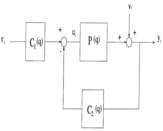
We will use a two degree of freedom controller in the configuration shown in Figure 3.1. This will supply a control input of the form

« ( 0 =

Ci(q)r{t) - C

(q)y(l)

Here Ci{q) and 6*2(9) controllers of predetermined type such as FIR filter

or PID controller and the design procedure involves the determination of the parameters of these controllers giving the best performance in terms of the

LQG cost function Jlqg

Vi

. 1

Figure 3.1: LQG Control System.

Now inserting the control input expression in Eqn. 3.1, we obtain

1

1 + P { q ) C2{ q ) ^ ^ 1 + P { q ) C , { q ) Similarly inserting this in Eqn. 3.3 we get

v ( t ) (3.4) ^ C M , 1 + P { q ) C2{ q ) --- ---1 + P ( q ) C2{ q ) v { t ) . (3.5)

Based on these equations the following lemma will give the frequency domain

evaluation of Jlqg, which will be crucial in the development.

L e m m a 3.1 : F o r t h e c o n f i g u r a t i o n o f F i g u r e 3 . 1 , i f t h e t r a n s f e r f u n c t i o n s b e t w e e n a n y t w o o f t h e s i g n a l s i n t h e s y s t e m a r e a l l s t a b l e a n d i f r a n d v a r e u n c o r r e l a t e d , t h e n t h e L Q G c o s t f u n c t i o n c a n be f o u n d a s 1 1 P C 2 - \ \ ‘ + \ \ C , W , . l + A|C2p ^ , II + P C2I2 II + P C2I2

P r o o f : W ith the error signal defined as

1 + P(l)Cii<l)

Referring to Eqn. 2.18, we see that

Jl q g — ^ e ( O ) + A R„0 ,

which is equivalent to

1 /■2’r 1

Jlqg = ^ 7o ’

remembering that the autocorrelation is the inverse fourier transform of the

power spectrum (see Eqn. 2.22). With the help o f the relations given in

Theorem 2.3 and the fact that r and v are uncorrelated (which allows us to

treat the summation of r and v terms independently) we can find that

^ , | P C i - P C2- i p ^ , , , 1 ^ ,

|l + PC'2l2 II + P C2P

Inserting these we can easily obtain the expression given in Eqn. 3.6. □

R e m a r k : In Chapter 2, we used as an index in the transfer function of the system. In the previous lemma, we used a; rather than e·'*^ as an index of the transfer functions. This is only a simplification of notation and it will be used in the present and next chapters. □

Denoting the parameter vectors of the controllers by 0 i and O2, we can

formulate the problem as the minimization of Jl q g with respect to 61 and 62. We assume that the controller transfer functions can be expressed as

C(q) = c'(q)» ,

where 9 is the parameter vector of the controller and and c(^)is the vector

showing the structure of it. For PID controllers and F^IR filters we have

Cpwiq) = Kp + IQ{1 - q-^) + K i{l - CpiRiq) =

^1

(3.8)

(3.9)

Hence we can use Eqn. 3.7 for PID and FIR type controllers with

c p i o i q )

--1

There may be other types of pararnetrizations for the other types of controllers. In this work we will develop our ideas for the types of controllers which can be represented through the use o f Eqn. 3.7. For these types of controllers utilized in the control system, the following lemma states the main result of this work.

L e m m a 3.2 : L e t t h e a s s u m p t i o n s o f L e m m a 3 . 1 h o l d . A s s u m e t h a t t h e f i r s t c o n t r o l l e r c a n be e x p r e s s e d t h r o u g h t h e u s e o f E q n . 3 . 7 . T h e n t h e o p t i m a l p a r a m e t e r v e c t o r o f t h e f i r s t c o n t r o l l e r 9°^ i s r e l a t e d t o t h e o p t i m a l p a r a m e t e r o f t h e s e c o n d c o n t r o l l e r 62 a s w h e r e A { 9 ° ) 9 \ = Ц Ѳ І ) , (3.12) A = 1 /*2^ Л -f" I 2тг Jo |1 + P { u } ) C2{ ^ ) \ ^ Фг(о;) Ci(a;)Ci (w) do: , (.3.13) b = 1 /‘2’f rZTT Jo

T

Р{ш)

C ”

PCiiS,)

Proof : The optimal solution is found through the use of the equations

; ^ І е г о ­

dC(q)

д \С Щ

дѳ

дѲ

дС(д)

дѲ

СЧ?) +

_дв

where denotes the real part. Then we can determine the gradients using Eqn. 3.6. However initially, it will be useful to see that,

\ P C i - P C \ - Ip { P C i - P C2 - 1 ) { P ’ C : - P ^ c : - n { I + P C 2 ) { \ + p - c ^ )

|i + P C2I2

^ P C \ p - c i

II + PC2I2 I + PC2 l + P’Q ·

Hence, Eqn. 3.6 is equivalent to

, _ L r r n _ . g + i m i C i p . ^ , , 1 + A|C,P ,

2 n J a **h + P C2* ’^ II + P C2P * |1+ P C2P * " * “ ‘ Then we can obtain the first gradient as

d J ,LQG 8 0 1

Equating to zero and noting that the integrals are already real (because of the conjugate symmetry of the transfer functions), we end up with Eqn. 3.12.

Note that the second derivative of Jlqg with respect to 6\ is equal to the

matrix A , which is a positive definite matrix for a reference input of continuous spectrum. If the reference input has nonzero power at finitely many frequencies, then it will again be positive definite if the number of parameters of the first controller is less than two times the number of different frequencies of the reference signal. This is because the positive definiteness condition drops down to the condition that the unique solution of a homogenous system of equations should be the zero vector, and this is the case under the mentioned situation (for the other case, the problem is analysed explicitly in the next section). This result guarantees that the solution of Eqn. 3.12 gives the minimum. Thus given

that the optimal parameter vector o f the second controller is solution of

Ecjn. 3.12 gives the optimal parameter 6\ of the first controller. Then premultiplying Eqn. 3.12 with 0 j, we see that

/•2TT

L

Using these equations we can reduce the cost function to Ji q q- O

Lemma 3.2 is useful as it reduces the optimization with respect to and

02 to an optimization with respect to $2 only. Thus a numerical optimization

algorithm, searching only the optimum value of B i can be utilized to design the optimal control system. Such a method will be presented in the next chapter.

3.4

Tracking the Reference Signals of Finite

Frequency Content

As observed from Eqn. 3.12, the power spectrum of the reference input deter­

mines the exact form of the optimality relation between the parameter vectors. It is an immediate study to search for certain results for the cases of special types of reference inputs. The following theorem gives a result for the case of reference inputs which have nonzero power at finite number of frequencies and is one of the mains contributions of this thesis.

T h e o r e m 3.1 : L t t P be a s t a b l e s y s t e m r e p r e s e n t e d b y E q n . 3 . 1 i n w h i c h v [ t ) — 0,Vi ( z e r o d i s t u r b a n c e c a s e ) . L e t C \ be a n F I R f i l t e r o f l e n g t h n \ . A s s u m e t h a t t h e r e f e r e n c e i n p u t h a s n o n z e r o p o w e r a t I d i f f e r e n t f r e q u e n c i e s ( e s s e n t i a l f r e q u e n c i e s a r e i n [0,7t] f o r r e a l s i g n a l s b e c a u s e o f t h e s y m m e t r y o f t h e p o w e r s p e c t r u m ) . I n t h i s c a s e , i f n \ > 21 t h e n f o r a n y s t a b i l i z i n g c o n t r o l l e r C2, t h e s o l u t i o n o f E q n . 3 . 1 2 r e s u l t s i n a c o n t r o l s y s t e m w h i c h i s o p t i 7 n a l a n d t h e o p t i m a l c o s t i s Jmin — A 2 i r ^ ^ X + \ P { u J k W

Here denotes the weigths of the impulses at ujk.

cko (.3.16)

P r o o f : If a reference input has nonzero power at u>k, then it has the same

amount of power at 27t— uJk- Hence, Eqn. 3.12 reduces to

where

'Y^[(f){i^k)cFlR {^k) + <?i>(27r - o:k)cFiii{2T r - u;^)] = 0 ,

k=i

I1 + PC2I2

1 + PC2·

Using the conjugate symmetry of the transfer functions we obtain

i

^ ^ { ( f > { u k ) c F r R ( i ^ k ) } — 0 ,

k=l

which can be organized as the following system of equations.

1 0

C O S U > i s i n w i

1 0

COS

(JL

>1

cos(n i—2)u;i sin(ni—2)o;i · · · cos(n i—2)o;/ sin(ni—2)oj; cos(ni—Ijwi sin(ni—l)u;i ··· cos(ni—l)u;/ sin(ni—l)u;;

0 0

0 0

where 3? and 5 denote the real and imaginary parts respectively. This is a

homogenous sytem with 21 unknown and r i i equations. The equations are in­

dependent because of the eigenfunction property of the functions This

can also be seen by noting that the complex form of the matrix above is related to the Vandermonde matrix (see [22]) with A, = e·'"·. It can be easily seen that this matrix has full column rank as w,s are different. Hence the unique solution of this system is the zero vector if ni > 21 [22]. Thus for r ii > 2/, (f>{u>k) will be zero for all k which means for each u,'k we will have

p I _ (A + | F P )Q I

l+PC2'"''‘

II + PC2P

Manipulating this we can find P*(1 + P C ,) U Л + |pp ■ Hence P C , |pp . 1 + P C2 A + |P|2 ·

Using Eqn. 3.15 we conclude that the value of the cost function is given by Eqn. 3.16, which is independent of C2· This means that for any stabilizing C2·,

Eqn. 3.12 gives an optimal solution which results in a minimum cost given by

Eqn. 3.16. □

R e m a r k : For the special cases where u>k = 0 or тг, the 2^-th column can be

removed together with ^ ф { и к ) from the system of equations. Thus the min­

imum number of parameters needed for the optimality situation described in

Theorem 3.1 should be found by counting one for frequencies 0, ж and two for

the other. □

The result of Theorem 3.1 reduces the minimization problem, to the mini­ mization of Jdr LQG 1 C - Х + \ С 2 { в 2 ) \ ‘ _ 1

~ ^ Jo

IT

with respect to 62 , for the case where the disturbance acting on the system is nonzero.

Periodic signals have nonzero power at finitely many frequencies related with the period of the signal. Thus Theorem 3.1 is applicable to the tracking of periodic reference inputs.

For smaller n , than needed, there is an optimal 62 which gives the best

result. Intuitively a value of 02 resulting in a transfer function whose

real part is near to 1 at the essential frequencies of the reference input will give a good result. This may be a useful observation especially in a numerical algorithm, to start from a good enough initial estimate.

Chapter 4

ONLINE DESIGN OF

IDENTIFICATION AND

CONTROL

As noted previously, many control design techniques are based on the model of the plant to be controlled. For plants o f unknown dynamics a model is estimated (possibly with a bound on the magnitude of the estimation error) and a controller is designed accordingly. Robust control and robust stability theory deals with the performance of the designed controller when applied on the actual plant.

In most practical applications of modern control, an initial controller is to be refined using online performance measurements in order to achieve better results in terms of the predetermined control purpose. Thus identification and control design have to be treated as a joint problem instead of two individual problems [10, 28]. Solution of this problem during online operation necessitcvtes the use of an iterative scheme composed of approximate identification and model based control design stages [28].

There are several iterative schemes proposed in the literature. In [.33] and the related works [25, 34], a paradigm is developed for LQG control design together with prediction error identihcation. In the proposed algorithms, the modelling error is taken into account during the control design through fre- ciuency weighting the LQG criterion and the identification is performed using the filtered versions of the identifier signals in order to match the requirements of the closed loop controller. The scheme of [29] is composed of a robust con­ trol design method and a frequency domain identification technique based on coprime factorization. Alternatively in [19], identification and control design are based on covariance data and the q-Markov cover theory is utilized.

In this chapter we will present our scheme, which is the combination of frequency domain identification through the use of the ETFE and parameter optimized design of controllers through numerical optimization and the opti­ mality relation found in the previous chapter.

4.1

Iterative Design of Identification and

Control

P r o b le m S t a t e m e n t : Let P be a stable and causal LTI system described by Eqn. 3.1. The dynamics of the system is unknown and we are to design controllers C \ and C2 (see Figure 3.1) during online operation such that Jl q g

given by Eqn. 3.2 is minimized, for a given reference signal with power spectral density $r·

P r o p o s e d A lg o rith m : The algorithm we will present is basically an it­ erative search algorithm, composed of the estimation of the transfer function of the plant and utilization of this transfer function in the design of the controllers based on the optimality relation (3.12). It can be described as follows.

Initially the system is operated with C \ = \ and C2 = 0 and input/output

data are collected. The controllers are updated after each N steps of operation.

The identification and control design steps and update rules can be summarized as follows.

Identification :

The idea is based on the smoothing method described in Section 2.4. Based on = Vn - ' W u H - ' ' { k ) · , (4.1) 1 K ( i ^ ) = (4.3) ( ¿ + l ) i V - l K { k ) - y : ^ [ i г N - N + l ) K , . d k ) + E \ U h \ k ) \ ^ ] (4.4) ^ t = i N yt =

0

1

the transfer function estimate at the ¿th step is

h M =

^ u . { k )

A; = 0, l , . . . , A f - l . (4.5)

Note that this estimate is an improved estimate according to Eqn. 2.29. On the other hand, ^ y u i { k ) and ^ u i { k ) are the estimates of the cross spectrum of y with u and spectrum of u at the fth step respectively. So the estimate can also be seen as an application of Blackman-Tuckey procedure without the use of a frequency window.

Control Design and Update Rules :

The update of the second controller is performed according to the kept record of the cost function estimate based on the system data observed in the intervals of length N .

Ji =

I (i+l)/v-l

N _{t = i N}E [ » W - ’- i o r + A U w r (4.6) J ° is the optimal value of J ' that occured till the current time and $2 is the corresponding parameter vector of the second controller. They are updated according to

i f J i < J ° e°2 = 02, a n d J ° = J '

The parameter vector of the second controller that will be used in the next step of operation is then determined as

^2. = ^2 + ^^2.+i (4.7)

where is a disturbance vector whose norm is equal to a percent of 62

(plus a small value for B2 equal to the zero vector). This disturbance can be a random disturbance as well as a deterministic one, based, for example, on the estimate of the gradient at the present parameter values (gradient descent algorithm). Similarly it can also be adjusted according to the performance of the previous controller with respect to the optimal controller determined till that time. Initially J ° = Jo and B2 = 0. The disturbance vector can be

assigned to zero with the achievement of an acceptable J ° or it can be reduced

to zero gradually with time, expecting convergence to the optimal value of the second controller.

The controller C \ is determined according to an approximate version of

Eqn. 3.12. Ai+l = b,q.i (4.8) Ai'+i bi+l N - l = E \ + \Pi(LOk)\" k=o + P i { ^ k ) C2i^i{u:k)\" A^-1 = E Pi{<^k) k=0 i + ^¿(Wfc)C'2i+i(i^A:) ^r(wA:) Ci(u;A:) (4.10) 34

In case of the loss of stability and with a (necessarily) large N , the algoritrn will have a problem. Thus a stability check should be added. A simple one is to check the ratio of the absolute value of the output to the maximum value of the absolute value of the reference input. If the ratio becomes greater than a predetermined value (this should be large enough such that the stable loops are not determined as unstable and it should be small enough such that the system is not destroyed), the algorithm should be reset (or the controllers should be updated realizing the optimal ones that have been determined till that time).

4.2

Alternative Algorithms

Dealing with real signals, we are assured that the DFTs are conjugate symmet­

ric around N / 2 (with N even). So the formulae can be reorganized and new

ones utilizing only the N / 2 -f 1 essential values of the transfer functions can be obtained. This is a quite important reduction for practical applications.

Moreover, with different length of adaptation intervals the transfer func­

tions (transfer fuction from C i { q ) r to y ) and (transfer friction

from Ci(<3')r to u) can be estimated and the optimality relation can be realized through the use of these estimates.

As noted, all of these involve the calculation of the N point DFTs of the

signals. An alternative algorithm can be offered if the optimality relation (3.12) is carefully analysed.The following lemma gives the basic idea.

L e m m a : W i t h t h e s y s t e m o p e r a t i n g w i t h Ci = 1 a n d C2, a n d w i t h z e r o d i s t u r b a n c e a s s u m e d , A a n d b o f E q n . 3 . 1 2 c a n be f o u n d a s

A = [ a m n ] \ a m n = >^Ru{n - m ) + R y { n - m ) ■, m, n = 1 , . . . , Ui.(4.11)

b — \bm\ 5 — R y r(1 ^ ) i ^ l , . . . , n i . (4.12)

P r o o f : With Cl = 1, we have from Eqns. 3.4 and 3.5 that

y(i) =

j-+ P C2

“<'> = rTW”·''’ ■

^'•|1 + PC'2|2 + p

— --- = $ ’^l + PC'2

Note that Ci(i<;)cj’ ('iu) is a matrix [cmn] with Cmn = Hence the inte­

grals in Eqns. 3.13 and 3.14 give the elements of A and b as

1

These are the inverse Fourier transforms according to Eqns. 2.22 and 2.23, hence the statement of the lemma follows. □

Lemma 4.1 gives the basic idea of a method omitting the explicit identifica­ tion step. Instead, the optimality relation can be realized through the estimates of A and b based on the correlation function estimates obtained from the data of the closed loop operated with C \ = 1. Thus in an alternative algorithm, the closed loop can be operated with Cj = 1 for A steps in order to determine the optimal C l for the current C2 and this optimal value can be used in the closed

loop in the following N steps of operation for the realization of the numerical

optimization algorithm.

There can also be different approaches to the numerical optimization part. One immediate approach is the utilization of the frequency domain evaluation of the cost function. In this case also, the stability of the closed loop has to be tracked, because this evaluation is valid for the case of stability. The aventage of this approach is that one can use shorter adaptation intervals. However the practical evaluation of the cost function in the frequency domain can have large errors which can cause certain problems.