Macroeconomics and the Term Structure
Refet S. Gürkaynak
yJonathan H. Wright
zFirst Draft: April 2010
This version: September 12, 2010
Abstract
This paper provides an overview of the analysis of the term structure of interest rates with a special emphasis on recent developments at the intersection of macroeconomics and …nance. The topic is important to investors and also to policymakers, who wish to extract macroeconomic expectations from longer-term interest rates, and take actions to in‡uence those rates. The simplest model of the term structure is the expectations hypothesis, which posits that long-term interest rates are expectations of future average short-term rates. In this paper, we show that many features of the con…guration of interest rates are puzzling from the per-spective of the expectations hypothesis. We review models that explain these anomalies using time-varying risk premia. Although the quest for the fundamental macroeconomic explanations of these risk premia is ongo-ing, in‡ation uncertainty seems to play a large role. Finally, while modern …nance theory prices bonds and other assets in a single uni…ed framework, we also consider an earlier approach based on segmented markets. Mar-ket segmentation seems important to understand the term structure of interest rates during the recent …nancial crisis.
JEL Classi…cation: C32, E43, E44, E58, G12.
Keywords: Term structure, interest rates, expectations hypothesis, a¢ ne models, in‡ation, …nancial crisis, segmented markets.
We are very grateful to Roger Gordon and three anonymous reviewers for their very helpful comments on various drafts of this paper. All errors and omissions are our own responsbility alone.
yDepartment of Economics, Bilkent University, 06800 Ankara, Turkey and CEPR. [email protected].
zDepartment of Economics, Johns Hopkins University, Baltimore MD 21218. [email protected].
1
Introduction
On June 29, 2004, the day before the Federal Open Market Committee (FOMC) began its most recent tightening cycle, the overnight interest rate, the federal funds target, was one percent and the ten-year yield was 4.97 percent. On June 29, 2005, the corresponding rates were three percent and 4.07 percent. Over the course of a year when the Fed was tightening monetary policy, increas-ing the overnight rate by 2 percentage points, longer-term yields had instead fallen. The ten-year rate decreased by 90 basis points. Fixed mortgage rates and longer-term corporate bond yields fell even more. This rotation of the yield curve surprised then Fed Chairman Greenspan. In his oft-quoted February 2005 testimony to Congress, he stated:
“This development contrasts with most experience, which sug-gests that ...increasing short-term interest rates are normally ac-companied by a rise in longer-term yields. . . For the moment, the broadly unanticipated behavior of world bond markets remains a conundrum.”
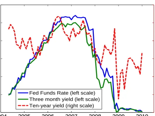
But similar patterns in the con…guration of interest rates have happened before— and since. Figure 1 shows the federal funds rate, three-month Treasury bill yields, and ten-year Treasury yields over the last seven years. The federal funds rate and three-month yields moved closely together, but ten-year (and other long-term) yields were often uncoupled from short-term rates. Greenspan’s co-nundrum is one example. Another is that in the early fall of 2008, as the FOMC was cutting the federal funds rate sharply, long-term interest rates actually rose, peaking in early November of that year. This could be called the “conundrum in reverse.” Later on, long-term yields declined sharply, around the time that the Fed announced the start of large-scale asset purchases.
The object of this paper is to discuss work on the macroeconomic forces that shape the term structure of interest rates. Broadly, the explanations fall into two categories. The …rst is that long-term interest rates re‡ect expectations of future short-term interest rates. This is the expectations hypothesis of the term structure of interest rates. If short-term interest rates are in turn driven by in‡ation and the output gap, as in the Taylor rule, then the term structure of interest rates ought to re‡ect expectations of future in‡ation and the output gap. For example, if the FOMC lowers policy rates today but, because of higher expected in‡ation, this leads agents to anticipate higher short-term interest rates in the future, then long-term interest rates could actually increase. The second category of explanations argues that long-term interest rates are also a¤ected by risk premia, or by the e¤ects of market segmentation, which can break the link between long-term interest rates and expectations of future short rates.
The literature on term structure modeling is vast. This paper portrays the state of that literature by presenting di¤erent theories in a uni…ed framework. We look at which aspects of the data are explained by di¤erent models using term structure data from 1971 to the present, and discuss the macroeconomic foundations and implications of the di¤erent models. Our aim is to focus on interactions between macroeconomics, monetary policy, and the term structure, rather than to consider term structure models from a more technical …nance perspective. Comprehensive reviews of the latter variety are already available in Du¢ e (2001), Singleton (2006) and Piazzesi (2008).
There are many reasons why policy-makers, investors and academic econo-mists should and do care about the forces that a¤ect the term structure of interest rates. First, economists routinely attempt to reverse-engineer mar-ket expectations of future interest rates, in‡ation, and other macroeconomic variables from the yield curve, but accomplishing this task also requires us to
separate out any e¤ects of risk premia. For example, in early 2010, the yield-curve slope was quite steep. Some commentators suggested that this steep yield curve represented concerns about a potential pickup in in‡ation, but without more formal models, it is hard to know if this was right, or if other forces were at work instead. Second, analysis of the term structure has implications for how monetary policy ought to respond to changes in long-term interest rates. If long-term rates were to fall because of an exogenous fall in risk premia, then it seems natural that policy-makers ought to lean against the wind1 by
tighten-ing the stance of monetary policy to o¤set the additional stimulus to aggregate demand (McCallum (1994)). However the models that we shall discuss in this paper attempt to endogenize risk premia, and in this case the appropriate policy response is ambiguous and depends on the source of the change in risk premia (Rudebusch, Sack and Swanson (2007)). Third, at present, the federal funds rate is stuck at the zero bound. Monetary policy-makers may wish to pro-vide additional stimulus to the economy. Under the expectations hypothesis, the only way that they can do this is by in‡uencing market expectations of future monetary policy, perhaps by committing to keep the federal funds rate at zero for an extended period. On the other hand, if long-term interest rates are also bu¤eted by risk premia, then measures to alter those risk premia, per-haps through large-scale asset purchases, may be e¤ective as well. The Federal Reserve and some other central banks have recently tried this. Fourthly, under-standing the evolution of the term structure of rates is important for predicting asset returns and for determining the portfolio allocation choices of investors and their strategies for hedging interest rate risk. Finally, governments around the world borrow by issuing both short- and long-term debt, and debt that is
1The whole term structure of interest rates should be relevant for aggregate demand. For example, business …nancing involves a mix of short-term commercial paper and long-term corporate bonds. In the U.S.— though not in foreign countries— most mortgages are …xed-rate.
both nominal and index-linked (in‡ation protected). Understanding the market pricing of these di¤erent instruments is important in helping governments de-termine the best mix of securities to issue in order to keep debt servicing costs low and predictable.
The plan for the remainder of this paper is as follows. Section 2 describes basic yield curve concepts and gives some empirical facts about the term struc-ture of interest rates. Section 3 discusses the evidence on the expectations hypothesis of the term structure. Section 4 introduces a¢ ne term structure models, which the …nance literature has been developing over the last ten years or so as a potential alternative to the expectations hypothesis. Progress has been rapid, and these models provide an alternative in which long-term interest rates represent both expectations of future short term interest rates and a time varying risk premium, or term premium, to compensate risk-averse investors for the risk of capital loss on selling a long-term bond before maturity and/or the risk of the bond’s value being eroded by in‡ation. The models that are dis-cussed span a spectrum from reduced form statistical models to fully speci…ed structural dynamic stochastic general equilibrium (DSGE) models, and many intermediate cases. Section 5 examines the implications of structural breaks and learning for these models. Section 6 discusses term structure models with market segmentation, and section 7 concludes.
2
Basic Yield Curve Concepts and Stylized Facts
This section …rst introduces the basic bond pricing terminology that will be used in the remainder of the paper, and then presents the most salient stylized facts of the term structure of interest rates.
2.1
Basic yield curve concepts
The most basic building block of …xed income analysis is a default-risk-free zero-coupon bond. This security gives the holder the right to $1 in nominal terms at maturity, with no risk of default.2 Let P
t(n) denote the price of an n-year
zero-coupon bond at time t:
Pt(n) = exp( nyt(n))
where yt(n) is the annualized continuously compounded yield on this bond. This
bond pays the holder $1 at time t + n, and we can solve for the yield from t to t + n as:
yt(n) = n1ln(Pt(n))
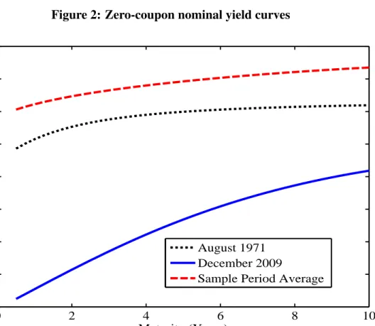
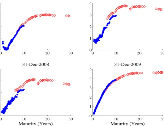
At any point in time, bonds of di¤erent maturities will have di¤erent yields. A yield curve is a function that maps maturities into yields at a given point in time. Graphically, it is a plot of yt(n) against n. Figure 2 shows the yield
curve out to ten years in the …rst and last months of our sample, as well as the average yield curves (i.e. the yields at each maturity averaged over the sample period). As is clear from the …gure, a stylized fact is that the yield curve slopes up on average. This has important repercussions for reverse engineering the yield curve to obtain expectations and term premia.
It is often more instructive to analyze long-term yields in terms of their constituent forward rates. The two-year yield observed today can be thought of as a one-year contract, with a commitment to roll over at a rate speci…ed today at the end of the …rst year. Since we observe the both the one-year and two-year yields, it should be possible to infer the rate implicitly agreed on today for the second year. This is a one-year-ahead one-year forward rate. More generally,
2We think of government bonds as being for all practical purposes free of nominal default risk but for some countries even sovereign debt may require modeling of default risk as well. And of course, the value of any nominal bond is always at risk of being eroded by in‡ation.
a forward rate is the yield that an investor would require today to make an investment over a speci…ed period in the future— for m years beginning n years hence. The continuously compounded return on that investment is the m-year forward rate beginning n years hence and is given by:
ft(n; m) = 1 mln( Pt(n + m) Pt(n) ) = 1 m((n + m)yt(n + m) nyt(n)) (1) Taking the limit of (1) as m goes to zero gives the instantaneous forward rate n years ahead, which represents the instantaneous return for a future date that an investor would demand today:
lim m!0ft(n; m) = ft(n; 0) = yt(n) + n @yt(n) @n = @nyt(n) @n = @ @nln(Pt(n)) (2) One can think of a zero-coupon bond as a string of forward rate agreements over the horizon of the investment, and the yield therefore has to equal the average of those forward rates. Speci…cally, from (2) we can write
yt(n) = n1 ni=1ft(i 1; 1) = n1R0nft(s; 0)ds
The beauty of forward rates is that they allow us to isolate long-term determi-nants of bond yields that are separate from the mechanical e¤ects of short-term interest rates.
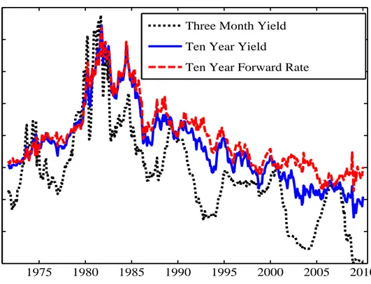
Figure 3 shows a long time series of three-month and ten-year yields, along with ten-year-ahead instantaneous forward rate in the U.S. Yields and forward rates generally drifted higher over the 1970s and then reversed course over the last thirty years, following the general pattern of in‡ation and longer-run in-‡ation expectations. But there was also much variation associated with the business cycle. Short-term interest rates were highly procyclical, as the FOMC sought to alter the stance of monetary policy to limit cyclical ‡uctuations in
in‡ation and output. On the other hand, forward rates were, if anything, coun-tercyclical.
In Figure 3, the usefulness of forward rates as an analytical device is evident at the end of 2009. Ten-year yields were at unusually low levels, by historical standards. However, long-term forward rates were somewhat above their average level over the previous decade; the unusually low level of long-term yields was solely the mechanical e¤ect of short-term interest rates being low, as the FOMC had set the federal funds rate to zero and expressed the intention of keeping it there for an extended period.
Another illustration of the usefulness of forward rates comes in looking at the e¤ects of macroeconomic news announcements on yields. Naturally, announce-ments of stronger-than-expected economic data cause interest rates to increase, as they presage a tighter stance of monetary policy. However, a more detailed analysis can be obtained by looking at the e¤ects of these announcements on the term structure of forward rates. Gürkaynak, Sack and Swanson (2005) …nd that stronger-than-expected economic data leads even ten-year-ahead forward rates to jump higher. This seems very unlikely to owe to any information about the state of the business cycle. A possible interpretation, proposed in that paper, is that long-term in‡ation expectations are poorly anchored. We return to this and alternative interpretations of the behavior of forward rates in section 4.
Another essential tool of term structure analysis is the holding period return. The holding period return is the return on buying an n-year zero-coupon bond at time t and then selling it, as an (n m)-year zero-coupon bond, at time t+m. This return is
hprt(n; m) = m1 [ln(Pt+m(n m) ln(Pt(n))]
and the di¤erence between this and the m-year yield is the excess holding period return:
exrt(n; m) = hprt(n; m) yt(m)
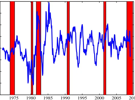
Figure 4 shows the excess holding period returns of the ten-year over one-year bonds over the sample period. These are on average positive— which follows from the average upward slope of the yield curve, shown in Figure 2— and also tend to be especially high at the beginning of recoveries from recessions. This is an important feature of the data that term structure models have to match.
2.2
The expectations hypothesis
The Expectations Hypothesis (EH) is the benchmark term structure model. In its strong form, it asserts that long-term yields are equal to the average of expected short-term interest rates until the maturity date. In its weak form, it allows for a constant term premium of the long yield over the average expected short-term interest rate. That term premium may be maturity-speci…c but does not change over time.
More formally, in its strong form, the EH states that investors price all bonds as though they were risk-neutral. That is, investors care only about expected outcomes (means of probability distributions), and will be indi¤erent between two assets with the same expected return but di¤erent levels of uncertainty. This implies that the price of an n-year zero-coupon bond is:
Pt(n) = Et(exp(
Z n 0
r(t + s)ds)) (3)
where r(t) = yt(0) is the instantaneous risk-free interest rate. Taking the logs
of both sides and neglecting a Jensen’s inequality term gives: yt(n) ' 1nEt(
Z n 0
r(t + s)ds)
because the log of an expectation is not the same as the expectation of a log— will tend to push long-term yields down, below the average of expected future short-term interest rates. This is the reason why at very long maturities (of about 20 years and longer), the yield curve typically slopes down. However, at maturities of about ten years or less, the Jensen’s inequality e¤ect is modest. For this reason, we neglect it henceforth in this paper as is customary in the literature.
Equivalently, in its strong form, the EH implies that instantaneous forward rates are equal to expectations of future short term interest rates:
ft(n; 0) = Et(r(t + n))
and that expected excess holding period returns are zero: Et(exrt(n; m)) = 0
The yield curve that would be realized with rational agents in the absence of arbitrage under risk neutrality is described by the expectations hypothesis, making it the natural benchmark for the study of the term structure of interest rates.
2.3
Risk premia and the pricing kernel
Economists generally believe that agents are risk-averse (see, for example, Fried-man and Savage (1948)). However, even under risk aversion, the pricing of dif-ferent contingent cash ‡ows has to be internally consistent to avoid arbitrage opportunities. More precisely, the absence of arbitrage implies that there exists a strictly positive random variable, Mt+1, called the stochastic discount factor
or the pricing kernel, such that the price of any asset at time t obeys the pricing relation:
where the price at time t + 1 includes any dividend or coupon payment that has been received. The stochastic discount factor is the extension of the ordinary discount factor to an environment with uncertainty and possibly risk-averse agents (see Hansen and Renault, 2009, for a detailed discussion of pricing ker-nels). Since the payo¤ of an n-year zero-coupon bond is deterministic and is equal to $1 at maturity, equation (4) implies that in period t + n 1, when the security has one year left to maturity, its price will be
Pt+n 1(1) = Et+n 1(Mt+n)
Iterating this backwards and using the law of iterated expectations, the bond price today will be
Pt(n) = Et(Qni=1Mt+i) (5)
Equation (5) makes no assumption of risk-neutrality and so does not imply that the EH holds. If risk-neutrality were to hold, then Mt+1 = Et(exp(
R1 0r(t +
s)ds)) and so equation (5) would collapse to equation (3), and long-term yields would be equal to the expected average future short-term interest rate as is the case under EH. But since we make no assumption of risk-neutrality, there may be a gap between long-term yields and the average expected future short-term interest rate. This is called the risk premium, or term premium:
rpt(n) = yt(n) n 1Et(Pn 1i=0 yt+i(1)) (6)
that compensates risk-averse investors for the possibility of capital loss on a long-term bond if it is sold before maturity and/or the risk of the bond’s value being eroded by in‡ation.3
3Although the payo¤ of a bond at maturity is known with certainty, the value of a long-term bond before maturity is uncertain. That is, the resale value of the bond before maturity (or the opportunity cost of funding the bond position) depends on the uncertain trajectory of future short term interest rates.
Equation (6) is e¤ectively an “accounting” de…nition of the risk premium— by construction, any change in long-term yields that is not accompanied by a corresponding shift in expectations of future short-term interest rates must result in a change in the risk premium. This could be a change in the risk premium from an asset pricing model (as will be considered in section 4), or it could result from the e¤ects of market segmentation (as discussed in section 6— a setup in which equations (4) and (5) do not apply). Any gap between yields and actual expectations is always de…ned as the risk (or term) premium.
2.4
Index-linked bonds
About thirty years ago, the United Kingdom started issuing index-linked bonds— government bonds with principal and coupons that are tied to the level of the consumer price index.4 These securities compensate the holder for the accrued
in‡ation from the time of issuance date to the time of payment date for each cash ‡ow date. The United States began the Treasury In‡ation Protected Secu-rities (TIPS) program in 1997, and many countries now o¤er index-linked debt to investors. Gürkaynak, Sack and Wright (2010) provide detailed information on the TIPS market.
The spread between nominal and indexed yields provides information on investors’ perceptions of future in‡ation, known as breakeven in‡ation5 or
in-‡ation compensation. Thus, the existence of inin-‡ation-indexed bonds has helped relate the nominal term structure to macroeconomic fundamentals by allowing for a decomposition of nominal yields into real and in‡ation-related components. But, just as investors’ pricing of nominal bonds may be distorted by risk pre-mia, the same is true for the pricing of index-linked bonds, and so both the real
4This was the …rst large-scale modern index-linked government bond market, although there is a centuries-long history of bonds that include some form of protection against in‡ation, such as being denominated in gold or silver.
5This spread is called breakeven in‡ation because it is the rate of in‡ation that, if realized, would leave an investor indi¤erent between holding a nominal or a TIPS security.
rates and breakeven in‡ation rates may be a¤ected by risk premia. We return to discuss these issues further in section 4 below.
3
Testing the Expectations Hypothesis
The expectations hypothesis is a natural starting point to study the term struc-ture of interest rates and also to relate macroeconomic fundamentals to the yield curve. Indeed, if the EH were su¢ cient to explain the term structure, then ex-pected short rates could be directly read from the yield curve. However, the fact that yield curves normally slope up is at odds with the simple EH because without term premia this would have to imply that short-term interest rates are expected to trend upwards inde…nitely. Therefore, the relevant form of the EH must be the weak from, which allows maturity speci…c term premia that are constant over time. This is how we de…ne the “expectations hypothesis”for the remainder of the paper.
Given its assumption of constant term premia, the EH attributes all changes in the yield curve to changes in expected short rates. As an accounting matter, the EH would imply that the 13
4 percentage point decline in long-term forward
rates from June 2004 to June 2005 must represent a fall of this magnitude in long-term expectations of in‡ation and/or the real short-term interest rate. It would also imply that the rebounds in forward rates during the early fall of 2008 and again in late 2009 represent increases in long-term expectations of in‡ation and/or real rates. Thus, under the EH, changes in the term structure can be used to infer changes in investors’ expectations concerning the path of monetary policy. If, in addition, the central bank’s rule relating monetary policy to macroeconomic conditions were known by those investors, then we could also read o¤ changes in their expectations of the state of the economy.
and point out some anomalies in the term structure, from the viewpoint of the EH, beginning with a very in‡uential approach proposed by Campbell and Shiller (1991). They proposed two tests which both test the implication of the EH that when the yield curve is steeper than usual, both short and long term rates must be expected to rise.6 Conversely, if the yield curve is ‡atter than
usual, short- and long-term rates must be expected to fall.
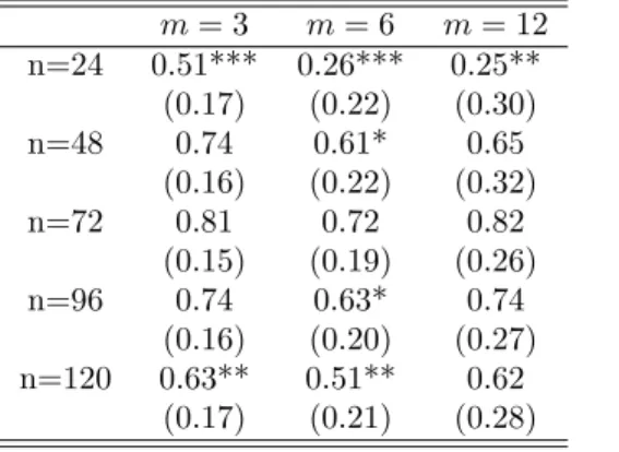
The …rst Campbell and Shiller (1991) test is based on the implication of the EH that the n-period interest rate is the expected average m-period interest rate over the next k = n=m intervals each of length m. That is, the return on lending for n periods today and the expected average return on lending for m periods and rolling over k 1 times should be equal:
yt(n) = k1Et( ki=01yt+im(m))
neglecting a constant. This means that
yt(n) yt(m) =k1Et( ki=01yt+im(m)) yt(m)
) yt(n) yt(m) = ki=11(1 ki)Et(yt+im(m) yt+(i 1)m(m))
and so if we consider the regression
k 1
i=1(1
i
k)(yt+im(m) yt+(i 1)m(m)) = + (yt(n) yt(m)) + "t (7)
which is a regression of a weighted-average of future short-term yield changes onto the slope of the term structure, then one ought to get a slope coe¢ cient that is equal to one. The dependent variable in equation (7) can be thought of as the perfect-foresight term spread, as it is the term spread that would prevail at time t if the path of period interest rates over the next m periods were correctly anticipated.
6Long rates as well as short rates are expected to increase when the yield curve is steep (under the EH) because with a steep yield curve distant-horizon forward rates are higher than short-term forward rates.
In Table 1, we report the results of the estimation of equation (7) using end-of-month U.S. yield curve data from the dataset of Gürkaynak, Sack and Wright (2007) from August 1971 to December 2009 for di¤erent choices of m and n. Newey-West standard errors with a lag truncation parameter of m are used, because the overlapping errors will induce a moving average structure in "t.
Like Campbell and Shiller (1991), we …nd that the point estimates of the slope coe¢ cient are all positive, but less than one. Some, but not all, are signi…cantly di¤erent from one. Overall this test gives only weak evidence against the EH.
The second Campbell and Shiller (1991) test is based on the implication of the EH that the expectation of the future interest rate from m to n periods hence is the forward rate over that period (again neglecting a constant). So
Et(yt+m(n m)) =n mn yt(n) n mm yt(m)
) Et(yt+m(n m) yt(n)) = n mm (yt(n) yt(m))
and, in the regression
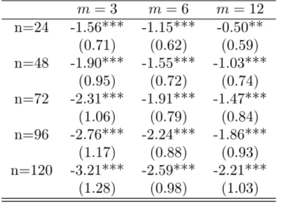
yt+m(n m) yt(n)) = + [
m
n m(yt(n) yt(m))] + "t (8) which is a regression of the change in long-term yields onto the slope of the term structure, the slope coe¢ cient should again be equal to one.
In Table 2, we report the results of the estimation of equation (8). Like Campbell and Shiller, we …nd that the estimates of are all negative and signi…cantly di¤erent from one, and become more negative as n increases. When the yield curve is steep, according to the EH, long-term interest rates should subsequently rise, but in fact they are more likely to fall. This term structure anomaly has been known for a long time, going back to MacAulay (1938). It is closely related to the …nding of Shiller (1979) that long-term yields are too
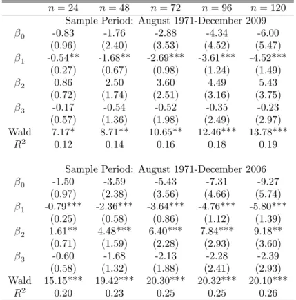
Another, related, approach to testing the EH was considered by Fama and Bliss (1987), Backus, Foresi, Mozumdar and Wu (2001), Du¤ee (2002) and Cochrane and Piazzesi (2005, 2008). This involves regressing the excess returns on holding an n-year bond for a holding period of m years over the return on holding an m-year bond for that same period onto the term structure of interest rates at the start of the holding period. Under the EH, term premia are time-invariant, and so ex-ante expected excess returns should be constant, and all of the coe¢ cients on the right-hand-side variables should jointly be equal to zero. For example, following Cochrane and Piazzesi (2008), one could regress ex-cess returns on holding a …ve-year bond for one year over the return on holding a one-year bond onto one-year forward rates ending one, three, and …ve years hence, estimating the regression:
exrt(n; 1) = 0+ 1yt(1) + 2ft(2; 1) + 3ft(4; 1) + "t (9)
This is a regression of the excess returns that are realized over the year on observed forward rates at the beginning of the year. The EH predicts that the slope coe¢ cients should all be equal to zero. The coe¢ cients from estimating equation (9) over the sample period from August 1971 to December 2009 are shown in Table 3. Again the EH is rejected. According to the EH, none of the forward-rates on the right-hand-side should have any predictive power for excess returns. But the R2values for this regression range from 12 to 20 percent.
Table 3 also shows the results from estimating this regression over a period that excludes the recent …nancial crisis (August 1971 to December 2006). For this earlier period, the rejection of the EH is even more decisive.
There is thus a good bit of evidence of anomalies in the term structure that the EH cannot account for. But a number of caveats should be pointed out with this assessment. First, there are econometric issues associated with
estimating equations (8) and (9) with relatively short spans of data. Both are regressions relating quite persistent variables, and ordinary distribution theory often provides a poor guide to the small sample properties of estimators and test statistics under these circumstances. It’s a bit like running a regression of one trending variable on another, which has the well-known potential to result in a spurious regression. Also, the regressions are subject to the possibility of peso problems in which yields are priced allowing for the possibility of a regime shift that was not actually observed in the short sample. Bekaert and Hodrick (2001) and Bekaert, Hodrick and Marshall (2001) both consider the two tests of Campbell and Shiller (1991), but provide alternative critical values that are more appropriate in small samples, given these problems. Even with these adjustments, they continue to reject the EH, although less strongly.
Second, some authors have examined evidence on the expectations hypothe-sis for very short maturity bonds and obtained mixed results. Rudebusch (1995) and Longsta¤ (2000) considered regressions of the form of equations (8) and (9) where the maturity of the “long bond” is measured in days or weeks. Little evidence is found against the EH. However, Piazzesi and Swanson (2008) con-ducted a similar exercise with short-term federal funds futures, and rejected the EH.
Third, Froot (1989) considered a di¤erent approach to testing the expecta-tions hypothesis. He compared forward rates with survey-based expectaexpecta-tions of future interest rates. For short-term rates, the two diverged, indicating a failure of the EH. But for long-term rates, Froot found that the survey-based and forward rates agreed quite closely. The ‡ipside of this is that the errors in survey forecasts for interest rates seem to be quite easy to predict ahead of time, suggesting that the survey forecasts may not be fully rational (Bachetta, Mertens and van Wincoop (2010)). But it is consistent with the apparent failure
of the EH being in part due to agents’learning about structural changes in the economy.
Finally, most empirical work …nding problems with the expectations hypoth-esis has been conducted using post-war U.S. data. Authors considering earlier sample periods or other countries have obtained more mixed results. For ex-ample, Hardouvelis (1994) estimated equation (8) for all the G7 countries, and found that the evidence against the EH was much weaker for countries other than for the U.S.7 Mankiw and Miron (1986) estimated equation (7) over sample
periods from before the foundation of the Federal Reserve system in 1914 and found support for the EH. Overall, the sample periods or countries for which the EH …nds most support are ones during which long-run in‡ation expecta-tions were presumably well anchored, such as the U.S. under the gold standard or countries such as Germany and Switzerland that held in‡ation in check even in the late 1970s. And the cases where the EH fares relatively poorly are ones with heightened in‡ation uncertainty and/or ones in which the central bank smoothed interest rates so that they are well approximated by a random walk speci…cation.
Overall there appear to be a number of features of the term structure of interest rates that the EH has trouble explaining. The standard …nance expla-nation is that this is due to time-variation in risk premia. In the next section, we turn to models with time-varying risk premia and ask what information about macroeconomic fundamentals can be uncovered by separating expected short rates from time-varying term premia. But the anomalies could owe in part to changes in long-run in‡ation expectations about which agents learn slowly. Accordingly, we consider learning and structural change in section 5. We dis-cuss an approach advocated by Kozicki and Tinsley (2005) in which long-term
7Other authors …nding more support for the EH when applied to foreign countries include Gerlach and Smets (1997), Jondeau and Ricart (1999), Bekaert, Hodrick and Marshall (2001) and Bekaert, Wei and Xing (2007).
interest rates are given by agents’ beliefs about average expected future short rates— and so the EH holds after all— but where these beliefs are conditioned on agents’perceptions of the central bank’s long-run in‡ation target, not the true in‡ation target. The agents’perceptions of the long-run in‡ation target are in turn formed by backward looking adaptive expectations. Kozicki and Tinsley argue that this model can explain many stylized facts of the term structure. Fi-nally, the con…guration of interest rates could re‡ect some market segmentation, a possibility that has generally been overlooked in the macro-…nance literature, but which we will consider in section 6. We argue that this approach may be helpful for understanding the behavior of long-term interest rates at times of unusual market turmoil, such as during the recent …nancial crisis.
We end this section by noting that researchers are now beginning to have enough data to obtain empirical evidence on the pricing of index-linked bonds. Evans (1997) and Barr and Campbell (1997) have applied tests of the EH to index-linked bonds in the U.K., with mixed results. Only a shorter span of data on in‡ation-protected bonds is available for the U.S., but with the available data it is striking how closely the long-term nominal and index-linked bond term structures track each other. Figure 5 shows the TIPS and nominal ten-year-ahead instantaneous forward rates. As can be seen in Figure 5, these two forward rates have moved almost in lockstep over the past ten years (see also Campbell, Shiller and Viceira (2009)).8 The TIPS market is still young and
less liquid than the nominal Treasury market, but this observation appears to suggest that a complete model of nominal term structure patterns will have to take account of real rate risk, as well as in‡ation risk.
8In other words, long-term forward breakeven in‡ation rates have been far more stable than long-term forward real rates.
4
A¢ ne Term Structure Models
A¢ ne term structure models provide an alternative to the expectations hypoth-esis.9 They have become enormously popular in the …nance literature in the last
ten years. A natural approach to term structure analysis would be to forecast interest rates at di¤erent maturities in a vector autoregression (VAR). Yields today are helpful for forecasting future yields (Campbell and Shiller (1991), Diebold and Li (2006) and Cochrane and Piazzesi (2005)), so this should be a viable approach to understanding how interest rates move over time. The trou-ble with this is that using the estimated VAR can— and typically will— imply that there is some clever way that investors can combine bonds of di¤erent ma-turities to form a portfolio that represents an arbitrage opportunity: positive returns without any risk. If we don’t believe that investors leave twenty dollar bills on the sidewalk, then it is important to exploit the predictability of future interest rates (from the VAR) in a framework that rules out the possibility of pure arbitrage. This is what a¢ ne term structure models do.
In this section we will lay out a¢ ne models with progressively more economic structure that will allow us not only to represent term premia statistically, but also to understand the economic forces at work. We will argue that the hedging of in‡ation risk is an important driver of bond risk premia. We will conclude the section with a short discussion of how index-linked bonds can be incorporated into the a¢ ne model framework.
The basic elements of a standard a¢ ne term structure model are as follows:
9A¢ ne models are models in which yields at all maturities are “a¢ ne” (linear plus a constant) functions of one or more factors. Most of the models discussed in this section are a¢ ne, but strictly speaking a few are models in which yields are instead nonlinear functions of the factors. While “factor-based term structure models” would have been a more precise section title, most of the models considered here are typically referred to as “a¢ ne” models. We thought it would be more helpful to introduce them as such.
(a) There is a kx1 vector of (observed or latent) factors that follows a VAR:
Xt+1= + Xt+ "t+1 (10)
where is "tiid N (0; I).
(b) The short-term interest rate is an “a¢ ne” (linear plus a constant) function of the factors:10
yt(1) = 0+ 01Xt (11)
(c) The pricing kernel is conditionally lognormal
Mt+1= exp( yt(1)
1 2
0
t t 0t"t+1) (12)
where t = 0+ 1Xt. Thus the set of factors that determine the short rate
also determine the long rates through the pricing kernel.
Langetieg (1980) showed that equations (5), (10), (11) and (12) imply that the price of an n-period zero-coupon bond is
Pt(n) = exp(An+ Bn0Xt) (13)
where Anis a scalar and Bn is a kx1 vector that together satisfy the recursions
An+1= 0+ An+ Bn0( 0) (14)
Bn+1= ( 1)0Bn 1 (15)
starting from A1 = 0 and B1 = 1. Zero-coupon yields are accordingly
1 0This model does not impose the zero-bound on interest rates. Kim (2008) discusses some extensions that do impose the zero bound.
given by yt(n) = An n B0 n n Xt (16)
This model is called an “a¢ ne” model, because yields at all maturities are all a¢ ne functions of the factors. Although other assumptions on the functional form of the pricing kernel and short-term interest rate are of course possible, the a¢ ne model is most popular in part because of its tractability.
If 0 = 1 = 0, then equations (5) and (11) imply that investors are
risk-neutral and the strong-form expectations hypothesis holds: Pt(n) = Etexp( n 1i=0yt+i(1)).
But we do not impose this restriction. The bond prices in equation (13) are how-ever the same as if agents were risk-neutral but the vector of factors followed the law of motion
Xt+1= + Xt+ "t+1 (17)
where = 0 and = 1 instead of equation (10). Equations
(10) and (17) are known as the physical and risk-neutral laws of motion for the factors, or P and Q measures, respectively. Intuitively, the risk-neutral law of motion uses a distorted data generating process, overweighting states of the world in which investors’marginal utility is high.
Many papers have estimated models of the form of equations (10) - (17). One very common approach is to infer the factors Xtfrom the current cross-section
of interest rates— the factors are either yields, or they are unobserved latent variables (see for example Du¢ e and Kan (1996), Dai and Singleton (2000, 2002), Du¤ee (2002), Kim and Orphanides (2005) and Kim and Wright (2005)). As three principal components are su¢ cient to account for nearly all of the cross-sectional variation in bond yields (Litterman and Scheinkman (1991)), most of these papers use three yield-curve factors in Xt, which can be interpreted as
(2007) consider an a¢ ne term structure model with three latent factors in which and are unrestricted, but = 0 and
= 0 B B B B @ 1 0 0 0 1 0 0 1 1 C C C C A
where is a parameter. Under these restrictions, equation (16) reduces to
yt(n) ' X1t+ X2t
1 exp( n= )
n= + X3t[
1 exp( n= )
n= exp( n= )] (18)
where Xt= (X1t; X2t; X3t)0is the state vector.11 This model has the appealing
feature that the yields follow the functional form of Nelson and Siegel (1987) that has been found to …t yield curves quite well— the elements of the state vector are just Nelson and Siegel’s level, slope, and curvature measures.
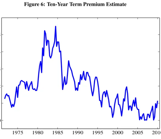
Term structure models with latent factors can be estimated by maximum likelihood using the Kalman …lter as in the model of Christensen, Diebold and Rudebusch (2007). Figure 6 shows estimates of ten-year term premia in the U.S. from this model.12 The term premium estimates rose in the 1970s, but
then trended lower from about 1985 to 2000. They tend to be countercyclical— higher in recessions than in expansions (Fama (1990) and Backus and Wright (2007)). Also, term premium estimates fell to the lowest levels in the sample in 2004 and 2005, o¤ering at least a partial explanation of Greenspan’s conundrum. Di¤erent models of course produce di¤erent estimates of term premia, but many of them agree on these points. Rudebusch, Sack and Swanson (2007) compare
1 1The model of Christensen, Diebold and Rudebusch is written in continuous time: here we are writing the discrete time representation of the law of motion of the state vector under the risk-neutral measure. Also note that equation (18) is an approximation, because it omits a remainder term that is time-invariant, and depends just on the bond maturity, n:
1 2We implement estimation of this model using end-of-quarter data on yields at maturities of 3 months, 6 months and 1, 2,....10 years. These yields are all assumed to be given by equation (18) plus iid N(0, 2
M E) measurement error. We specify that is a diagonal variance-covariance matrix. The parameters of the model are thus , , , 2 and the diagonal
…ve di¤erent term premium estimates and …nd that they all agree on some key points, particularly the downward trend in bond risk premia over the 1990s. We will return to the interpretation of this downward trend later. Judging from the Christensen, Diebold and Rudebusch model, term premia rose in 2009, although remained low by historical standards.
Approaches with either latent variables or yields as factors have the advan-tage of providing a close …t to observed interest rates using a small number of variables. But they have the drawback that they lack economic interpreta-tion. It would be hard to tell a policymaker that the key to having lower and more stable risk premia is to change the law of motion of some latent factor. The remainder of this section moves incrementally towards models with more economic structure.
4.1
Term structure models with macroeconomic factors
Some authors use macroeconomic variables as factors instead. Bernanke, Rein-hart and Sack (2004) use an a¢ ne model given by equations (10) - (17) in which the factors are GDP growth, in‡ation, the federal funds rate, and survey-expectations of future in‡ation and growth. Similarly, in Smith and Taylor (2009), the factors are in‡ation and the output gap. This means that short-term interest rates depend on in‡ation, t; and the output gap, gapt:yt(1) = 0+ 1;1 t+ 1;2gapt
Equation (16) then implies that yields at all maturities are a¢ ne functions of current in‡ation and the output gap:
yt(n) = a0(n) + a1(n) t+ a2(n)gapt
Smith and Taylor use the model to interpret yield curve movements. For exam-ple, they propose an interpretation of Greenspan’s conundrum, in which it owes
to the Fed being perceived to have lowered the sensitivity to in‡ation, 1;1, in
its Taylor rule. This caused the whole term structure of in‡ation response coef-…cients, a1(n) to move lower, and long-term yields declined, even as short-term
interest rates climbed.
Models with macroeconomic variables as factors allow the response of the yield curve to macroeconomic shocks to be analyzed. However, they do not …t observed yields quite as well as latent factor models. A possible approach is to combine both macroeconomic and latent variables as factors. Ang and Piazzesi (2003) provide a model in this category. They consider using as factors the …rst principal component of a set of in‡ation measures, the …rst principal component of a set of measures of real economic activity, and three latent factors. In the equation for the short-term interest rate (equation (11)), Ang and Piazzesi restrict the short rate to depend on in‡ation and economic activity alone, in as in the Taylor rule.
The inclusion of macroeconomic variables as factors raises two issues. Firstly, Ang and Piazzesi (2003) restrict the VAR in equation (10) so that the yield curve factors have no e¤ects on future in‡ation or output. Similar restrictions are im-posed by Hördahl, Tristani and Vestin (2006). The propagation of shocks is thus uni-directional. That seems a strong restriction, which in turn raises the question of why the central bank would want to adjust interest rates to in‡u-ence the macroeconomy. More recent papers have allowed for feedback between macroeconomic variables and yields. Diebold, Rudebusch and Aruoba (2006) consider a model with both yield curve and macroeconomic factors in which the VAR in equation (10) is unrestricted. Empirically, they …nd that yields a¤ect future values of the macroeconomic variables, and vice-versa. Nimark (2008) …nds that central banks using the information in yields about macroeconomic fundamentals can improve welfare.
There is a second and more thorny issue with the use of macroeconomic variables in a¢ ne models. Equation (16) relates the yield on an n-period bond to the factors. Using this equation for a set of di¤erent maturities gives a system of equations that one ought normally be able to use to solve for the factors from the observed yields. Thus, if macroeconomic variables are truly factors, then a regression of these variables onto yields ought to give a very good …t. However, regressing macroeconomic variables on yields consistently gives small to moderate R2 values. This point is made by Rudebusch and
Wu (2008), Joslin, Priebsch and Singleton (2009), Kim (2009), Orphanides and Wei (2010) and Ludvigson and Ng (2009). A way around this— proposed by Joslin, Priebsch and Singleton, Ludvigson and Ng, and Rudebusch and Wu— is to consider models in which knife-edge parameter restrictions are satis…ed, such that yields of all maturities have a loading of zero on the macroeconomic variables in equation (16). This means that there is a singularity whereby one cannot invert equation (16) to recover the macroeconomic variables from yields. This does not prevent yields from having forecasting power for future values of the macroeconomic variables. Changes in macro variables can a¤ect future yield curves and expectations of future short-term interest rates, but they have an o¤setting impact on term premia. The two e¤ects cancel out, leaving today’s term structure unchanged. The terminology used to describe this situation is that macroeconomic variables are unspanned factors.13
4.2
Structural models of factor dynamics
The term structure models considered up to this point use an unrestricted VAR in equation (10) to model the dynamics of the factors. And the stochastic discount factor is likewise driven by factors in an atheoretical way, given in
1 3Macroeconomic variables are not the only possible candidates for unspanned factors. Collin-Dufresne and Goldstein (2002) and Andersen and Benzoni (2008) argue that bond derivatives contain a factor that is not re‡ected in the term structure of yields.
equation (12). More structural approaches are however available in which the law of motion of the factors, or the stochastic discount factor, or both, are grounded in some economic model based on utility maximization.
This subsection considers models with the stochastic discount factor given by equation (12), but in which economic theory is used to motivate the law of motion of the factors. The economic theory could be a new-Keynesian macro-economic model, that in turn has micromacro-economic foundations. In this setup rather than an unrestricted VAR, the macroeconomic factors are driven by the model dynamics. In‡ation depends on expected future in‡ation, past in‡ation, and the output gap, in the hybrid new-Keynesian Phillips curve. Meanwhile, in the IS equation, the output gap depends on expectations of the future output gap, the past output gap, and the real short-term interest rate. Rudebusch and Wu (2007) is a model of this sort. The equations describing the evolution of these macroeconomic factors can be written as forward-looking linear di¤erence equations with rational expectations. Solution techniques for these equations have been proposed by a number of authors including Blanchard and Kahn (1980) and Sims (2001). The solution implies that the macro variables follow a restricted vector autoregression, that can however still be written in the form of equation (10). Other models in this family include Gallmeyer, Holli…eld, and Zin (2005) and Rudebusch, Swanson, and Wu (2006).
These models are better able to o¤er explanations grounded in economic theory for yield curve movements, as the driving factors are now restricted to behave in a model-consistent manner. However, the key ingredient of the model— the pricing kernel that maps the factors into yields— remains ad hoc. We now turn to models with pricing kernels that are based on utility maximization.
4.3
Risk premia from utility maximization
The models considered in this section so far are all able to match the empirical properties of the yield curve reasonably well. They get the slope of the yield curve right, and they match the anomalies documented by Campbell and Shiller (1991) and others. But they are based on a statistical model for the pricing kernel. That is, equation (12) is a reduced form expression for the pricing kernel that generates reasonable and tractable results, but the pricing kernel and the utility maximization that takes place in the macroeconomic model may not be consistent with each other. In this subsection, we now turn to discussing papers that have instead derived the pricing kernel from an explicit utility maximization problem, while going back to having unrestricted reduced form dynamics for the factors.
The …rst papers to analyze the term structure of interest rates with a struc-tural model of the pricing kernel had great di¢ culty in matching the most basic empirical properties of yield curves— notably that yield curves on average slope up indicating that nominal bond risk premia are typically positive. For example, Campbell (1986) considered an endowment economy in which consumption fol-lows an exogenous time series process and a representative agent trades bonds of di¤erent maturities and maximizes the power (or constant relative risk aversion) utility function
Et 1j=0 jc1
t+j
1 (19)
where ct denotes consumption at time t, is the discount factor and is the
coe¢ cient of relative risk aversion. The pricing kernel is therefore Mt+1 = ct+1
ct
which is the ratio of marginal utility tomorrow to marginal utility to-day. The term premium on bonds in this economy depends on the nature of the consumption process. If the exogenous consumption growth process is posi-tively autocorrelated, then risk premia on long-term bonds should be negative.
The intuition is that expected future consumption growth falls, and bond prices rise, in precisely the state of the world in which marginal utility is high. The long-term bond is therefore a good hedge, and the risk premium is negative. Therefore a positively autocorrelated consumption growth process would gener-ate negative risk premia. Conversely, a negatively autocorrelgener-ated consumption growth process would generate positive risk premia.
The problem with this story is however that consumption is close to being a random walk, implying that term premia should be close to zero. Thus these standard consumption-based explanations are hard to reconcile with the basic fact that yield curves ordinarily slope up. Backus, Gregory and Zin (1989) likewise discussed the di¢ culty of consumption based asset pricing models in matching the sign, magnitude and other properties of bond risk premia. Don-aldson, Johnson and Mehra (1990) and Den Haan (1995) were also unable to match the sign and magnitude of bond risk premia in real business cycle mod-els.14 Intuitively, the problem is that we generally think of recessions— periods
of high marginal utility— as times when interest rates fall causing bond prices to rise. This would make bonds a hedge, not a risky asset. The fact that bonds command a risk premium is therefore surprising; and often referred to as the “bond premium puzzle”. Resolving it requires a model in which the pricing kernel is negatively autocorrelated (Backus and Zin (1994)).
Piazzesi and Schneider (2006) and Bansal and Shaliastovich (2009) consid-ered another endowment economy model with a pricing kernel derived from util-ity maximization that does however account for positive term premia.15 Their
story is that it is in‡ation that makes nominal bonds risky, and this is indeed a
1 4Note that the models of Capmbell (1986), Donaldson, Johnson and Mehra (1990) and Den Haan (1995) are all silent on in‡ation. They are models that are concerned with the real part of the term structure.
1 5The model of Bansal and Shaliastovich (2009) has the additional feature of allowing the variance of shocks to change over time, which is appealing because one can di¤erentiate between changes in the “price” and “quantity” of risk.
recurrent theme of much recent work on the fundamental macroeconomic story that underlies bond risk premia. Piazzesi and Schneider show empirically that there is a low-frequency negative covariance between consumption growth and in‡ation.16 In‡ation therefore erodes the value of nominal bonds in precisely
those states of the world in which consumption growth is low and so marginal utility is high. The utility function that is used is that of Epstein and Zin (1989), which is an extension of the standard power utility function in equation (19) that breaks the link between the coe¢ cient of risk aversion and the intertem-poral elasticity of substitution implied by that utility function. Epstein-Zin preferences allow an individual to be both risk-averse and yet somewhat willing to smooth consumption intertemporally, which appears to better …t agents’be-havior. Using these preferences magni…es the premium that investors demand for the risk of in‡ation eroding the value of their nominal bonds at times when marginal utility is high, and so explains the large term premia that are observed in the data.
Since it is in‡ation that makes nominal bonds risky, the explanation of Pi-azzesi and Schneider (2006) and Bansal and Shaliastovich (2009) implies that while the nominal yield curve ought to slope up, the real yield curve should be roughly ‡at or even slope down. As pointed out by Piazzesi and Schneider, this matches the observed average slope of nominal and real yield curves in the U.K., but not in the U.S.17
Ulrich (2010) appeals to Knightian uncertainty to give a further twist on the role of in‡ation in pricing nominal bonds. He considers an endowment economy in which there is uncertainty about the data generating process for in‡ation.
1 6More precisely, consumption growth and in‡ation are both speci…ed to be the sum of their expected values plus noise. The expected values are assumed to be slowly varying. Piazzesi and Schneider (2006) use a Kalman …lter to estimate the covariance between the expected values of consumption growth and in‡ation, and …nd it to be negative.
1 7In the U.S., the TIPS yield curve is on average a bit ‡atter than its nominal counterpart, but it typically slopes up.
Faced with this model uncertainty, Ulrich follows the standard approach from the robust control literature, which is to suppose that agents assume the worst. That is, they price bonds assuming that in‡ation will be generated by whichever model minimizes their expected utilities. Not surprisingly, the e¤ect of this model uncertainty is to further raise the yields that investors require to induce them to hold nominal bonds.
Wachter (2006) considers another endowment economy with consumption growth and in‡ation as exogenous state variables, and explicit utility maxi-mization. The utility function is however di¤erent in that it incorporates habit formation. The investor’s utility function depends not on consumption as in equation (19) but rather on consumption relative to some reference level to which the agent has become accustomed. When calibrated using U.S. data, Wachter predicts that both nominal and real yield curves slope up. The intu-ition is that when consumption falls, investors wish to preserve their previous level of consumption and so the price of bonds goes down as marginal utility rises. This makes bonds (real or nominal) bad hedges, as they do badly when investors need them the most, and leads them to command positive risk pre-mia in equilibrium. Wachter also …nds that the model can match other term premium puzzles, notably the negative slope in the estimation of equation (8).
4.4
Structural models for the pricing kernel and factor
dynamics
Subsection 4.2 used structural models for the factor dynamics and a statistical representation for the pricing kernel. Subsection 4.3 did exactly the opposite. But recently some authors have used structural models for both the factor dy-namics and the pricing kernel, and this is the logical conclusion of a progression from atheoretical to structural models. For example, Bekaert, Cho and Moreno
(2010) combine a forward looking new-Keynesian model with a stochastic dis-count factor derived from maximizing utility in equation (19). The model is loglinear and lognormal, which makes it tractable to solve, but which however implies that the expectations hypothesis holds and that there is no term pre-mium (apart from the Jensen’s inequality e¤ect). A general problem with a structural model for both the pricing kernel and the factor dynamics is that it is challenging to maintain computational tractability and yet obtain time-variation in term premia.18
Rudebusch, Sack and Swanson (2007) and Rudebusch and Swanson (2008) do however model time-varying term premia in DSGE models with production using preferences with habit formation (as considered by Wachter (2006) in the context of an endowment economy). They …nd that the success that Wachter obtained in using habits to explain bond risk premia in an endowment economy does not extend to a DSGE model. The term premia in a habit-based DSGE model are very small. The intuition is that whereas in an endowment economy, agents facing a negative consumption shock will wish to sell bonds to smooth their consumption, in a production economy they can and will choose to raise their labor supply instead (Swanson, 2010).19
Rudebusch and Swanson (2009) did a similar exercise but using Epstein-Zin preferences instead. They had much more success in matching the basic empirical properties of the term structure. The intuition is an extension of that of Piazzesi and Schneider (2006) and Bansal and Shaliastovich (2008) to a
1 8These models require solution methods that are based on approximations around a non-stochastic steady-state. A …rst-order approximation delivers a zero term premium— it is as though agents were risk-neutral. A second-order approximation delivers a constant term pre-mium. Only with a third-order approximation, considered by Rudebusch, Sack and Swanson (2007), Rudebusch and Swanson (2008, 2009), Ravenna and Seppälä (2007) and Van Binsber-gen, Fernández-Villaverde, Koijen and Rubio-Ramírez (2008) does it become possible to have time-varying term premia.
1 9Alternatively, Rudebusch and Swanson (2008) can match the term premium in the habit-based DSGE model, but at the price of making real wages far more volatile than is actually the case in the data.
production economy: technology shocks cause consumption growth and in‡ation to move in opposite directions, meaning that in‡ation will erode the value of nominal bonds in precisely the state of the world when investors’marginal utility is high. This makes nominal bonds command a positive risk premium.
4.5
In‡ation hedging as the cause of term premia
The last two subsections have reviewed a range of macro-…nance term structure models in which the pricing kernel comes from an explicit utility-maximization problem. These models are all quite di¤erent. Yet many of them agree on one thing— in‡ation uncertainty makes nominal bonds risky. Although the search for fundamental macroeconomic-based explanations for term premia remains a work in progress, this does seem to be a pattern found by many authors.
If investors demand positive term premia to hedge against in‡ation risk, then we would expect in‡ation and consumption growth to move in opposite directions (as Piazzesi and Schneider (2006) and others have found empirically). We’d also expect a positive correlation between nominal bond returns and con-sumption growth, or other real-side measures. Campbell, Sunderam and Viceira (2007) found that the correlation between nominal bond returns and the real economy has varied over time, but was particularly high during the period of high in‡ation in the 1970s and early 1980s (the “Great In‡ation”). They also pointed out that the average slope of the yield curve has been unstable over time— yield curves tended to be fairly ‡at before the early 1970s, then became steep, and then ‡attened once again since the mid 1990s (see also Fama (2006)). Tellingly, these two shifts line up to some extent— the yield curve was steepest at the time when nominal bonds were especially risky assets. This pattern could indeed help to account for the bond premium puzzle, and for time-variation in term premia. According to this story, in the U.S. over most of the last few
decades, investors have mainly been concerned about supply shocks that shift the Phillips curve in and out, and they have consequently demanded positive bond risk premia. But the size, and even the sign, of bond risk premia depend on the economic environment. If investors were instead, at some times, more concerned about demand shocks shifting the economy along the Phillips curve, then they would view nominal bonds as a good hedge, and bond risk premia would be negative. Perhaps this helps explain the low level of bond yields in the summer of 2010— investors may have viewed bonds as a good hedge against the possibility of de‡ation and sustained economic weakness.
Piazzesi and Schneider (2006) also argued that term premia were particularly large during and immediately after the Great In‡ation, because the long-run correlation between in‡ation and consumption growth was especially negative at this time. Meanwhile, they argue that at other times, the relative importance of in‡ation shocks in the economy was smaller, and term premia were apparently lower. Palomino (2008) goes further back in time, and documents that the average term spread was negative in the U.S. under the Gold Standard from 1880 to 1932, which he interprets as evidence that the term premium re‡ects instability in long-term in‡ation expectations. The relatively favorable evidence on the expectations hypothesis from this period, and from other countries that arguably have more stable long-run in‡ation expectations (discussed in section 3 above), also supports this view.
Rudebusch, Swanson and Wu (2007) found that many a¢ ne term structure models showed a downward trend in estimated term premia over the course of the 1990s. This pattern is clearly visible in Figure 6 of this paper. A natural interpretation is that the 1990s were a time when in‡ation uncertainty was waning, again suggesting that in‡ation uncertainty is a key driver of bond risk premia.
There is yet more evidence to support this broad conclusion. A compelling example, is the market reaction to the announcement that the Bank of England was to be granted operational independence, on May 6, 1997. As documented by Gürkaynak, Levin and Swanson (2010) and Wright (2010), U.K. nominal yields fell sharply, and the nominal yield curve ‡attened dramatically, on the very day of this announcement. Meanwhile, real yields were little changed. It seems hard to account for this without appealing to the idea that a more stable nominal anchor lowered both in‡ation expectations and in‡ation risk premia.
On the other hand, a note of caution with respect to the view that in‡ation uncertainty is the cause of term premia is that this may be hard to reconcile with the patterns observed so far in the relatively new and comparatively illiquid U.S. TIPS market. Under this view, one might expect the real yield curve to be ‡at or to slope down, but in fact the TIPS yield curve typically slopes up. And long-term TIPS forward rates have moved almost in lockstep with their nominal counterparts (as shown in Figure 5).
4.6
A¢ ne models with both nominal and index-linked
bonds
A few recent papers have undertaken the ambitious but important task of ap-plying the a¢ ne model framework to nominal and index-linked bonds jointly. Let PREAL
t (n) be the real price of an index-linked zero-coupon n-period bond
at time t, and let Q(t) be the price level at time t: The analog of equation (5) is then:
PtREAL(n) = Et(Qni=1Mt+iREAL) (20)
where Mt+iREAL = Q(t+i 1)Q(t+i) Mt+i is the real pricing kernel. Coupled with an
ln(Q(t + 1)=Q(t)) = 0+ 01Xt+ t+1
where tis iid N (0; 2);20 (perhaps correlated with the factor innovations " t+1),
equation (20) implies that real yields will be an a¢ ne function of the state vector Xt, similar to equation (16). Several authors have …tted such a model
to nominal and TIPS yields jointly, including Buraschi and Jiltsov (2005), Kim (2004), D’Amico, Kim and Wei (2010) and Christensen, Lopez and Rudebusch (2010). In this way, in addition to having a decomposition of the nominal yield into nominal expected short rates and a nominal term premium, one can also decompose the real yield into real expected short rates and a real term premium. And then, as a matter of arithmetic, the di¤erence between these two is the decomposition of breakeven in‡ation21 into in‡ation expectations
and an in‡ation risk premium. In other words, the nominal yield is decomposed into four components: the expected real rate, expected in‡ation, the real risk premium and the in‡ation risk premium.
In the U.S., the TIPS market is tiny relative to the vast nominal Treasury market. At present, daily trading volumes in TIPS run at 1-2 percent of their nominal counterparts.22 Liquidity in the TIPS market was very poor in the years immediately following the launch of the TIPS program in 1997, and indeed at times there was talk of the index-linked bond issuance being discontinued in the United States. TIPS liquidity improved over the subsequent years, but then worsened sharply during the …nancial crisis (see, for example, Campbell, Shiller and Viceira (2009)). Investors surely demand a higher yield on TIPS to compensate them for this comparative lack of liquidity, and this liquidity premium must vary over time. In particular, it is impossible to rationalize the high level of TIPS yields during the …nancial crisis without appeal to a sizeable
2 0This represents a decomposition of in‡ation into expected in‡ation,
0+ 01Xt, and un-expected in‡ation, t.
2 1Recall that breakeven in‡ation is de…ned as the spread between comparable maturity nominal and real bond yields.
liquidity premium.23 D’Amico, Kim and Wei (2010) argue more broadly that a time-varying liquidity premium needs to be taken out of TIPS yields before using them to …t an a¢ ne term structure model. Such e¤orts will be especially useful when studying the behavior of real and in‡ation related components of the term structure during times of crises.
5
Learning about Structural Change
The models discussed in section 4 assume parameter constancy. And yet, these models are estimated over a period of time in which many macroeconomists believe that there were important changes in the economy, notably changes in the Fed’s implicit in‡ation target, that agents learned about slowly. Stock and Watson (2007) and Cogley, Primiceri and Sargent (2009) argue that the permanent component of U.S. in‡ation— or the Fed’s implicit in‡ation target— varied considerably over the last 40 years.
The idea that investors learn slowly about structural change has been incor-porated into models of the term structure. Indeed, some authors argue that this may account in large part for the apparent failure of the EH. For example, Koz-icki and Tinsley (2005) consider a model in which long-term interest rates are indeed given by agents’ beliefs about expected average future short rates, but in which these beliefs are conditioned on their perceptions of the central bank’s long-run-in‡ation target, not the true in‡ation target. These perceptions of the long-run in‡ation target are in turn formed by backward-looking adaptive expectations. This means that agents make systematic forecasting errors for in‡ation, and hence interest rates.24
2 3Certain TIPS real yields were noticeably above comparable maturity nominal yields at times during the fall of 2008. While low in‡ation expectations (and fear of de‡ation) no doubt contributed to this, the indexation adjustment to TIPS principal cannot be negative. For this reason, when TIPS yields are above their nominal counterparts, this can only represent a liquidity premium.