Optimal Stochastic Signaling for Power-Constrained
Binary Communications Systems
Cagri Goken, Student Member, IEEE, Sinan Gezici, Member, IEEE, and Orhan Arikan, Member, IEEE
Abstract—Optimal stochastic signaling is studied under second and fourth moment constraints for the detection of scalar-valued binary signals in additive noise channels. Sufficient conditions are obtained to specify when the use of stochastic signals instead of deterministic ones can or cannot improve the error performance of a given binary communications system. Also, statistical characterization of optimal signals is presented, and it is shown that an optimal stochastic signal can be represented by a randomization of at most three different signal levels. In addition, the power constraints achieved by optimal stochastic signals are specified under various conditions. Furthermore, two approaches for solving the optimal stochastic signaling problem are proposed; one based on particle swarm optimization (PSO) and the other based on convex relaxation of the original optimization problem. Finally, simulations are performed to investigate the theoretical results, and extensions of the results to𝑀-ary communications
systems and to other criteria than the average probability of error are discussed.
Index Terms—Detection, binary communications, additive noise channels, randomization, probability of error, optimization.
I. INTRODUCTION
I
N this paper, optimal signaling techniques are investigated for minimizing the average probability of error of a binary communications system under power constraints. Optimal signaling in the presence of zero-mean Gaussian noise has been studied extensively in the literature [1], [2]. It is shown that deterministic antipodal signals, i.e.,𝑆1= −𝑆0, minimize the average probability of error of a binary communications system in additive Gaussian noise channels when the average power of each signal is constrained by the same limit. In addition, for vector observations, selecting the deterministic signals along the eigenvector of the covariance matrix of the Gaussian noise corresponding to the minimum eigen-value minimizes the average probability of error under power constraints in the form of ∥S0∥2 ≤ 𝐴 and ∥S1∥2 ≤ 𝐴 [2, pp. 61–63]. In [3], optimal binary communications over additive white Gaussian noise (AWGN) channels are studied for nonequal prior probabilities under an average energy per bit constraint. It is shown that the optimal signaling scheme is on-off keying (OOK) for coherent detection when the signals have nonnegative correlation, and that the optimal signaling is OOK also for envelope detection for any signal correlation. In [4], a source-controlled turbo coding algorithm is proposedManuscript received June 16, 2009; revised March 11, 2010; accepted September 22, 2010. The associate editor coordinating the review of this paper and approving it for publication was M. Torlak.
The authors are with the Department of Electrical and Electronics Engi-neering, Bilkent University, Bilkent, Ankara 06800, Turkey e-mail: {goken, gezici, oarikan}@ee.bilkent.edu.tr.
Part of this research was presented at the IEEE International Workshop on Signal Processing Advances for Wireless Communications (SPAWC), Marrakech, Morocco, June 2010.
Digital Object Identifier 10.1109/TWC.2010.101810.090902
for nonuniform binary memoryless sources over AWGN chan-nels by utilizing asymmetric nonbinary signal constellations. Although the average probability of error expressions and optimal signaling techniques are well-known when the noise is Gaussian, the noise can have significantly different probability distribution from the Gaussian distribution in some cases due to effects such as multiuser interference and jamming [5]-[7]. In [8], additive noise channels with binary inputs and scalar outputs are studied, and the worst-case noise distribution is characterized. Specifically, it is shown that the least-favorable noise distribution that maximizes the average probability of error and minimizes the channel capacity is a mixture of discrete lattices [8]. A similar problem is considered in [9] for a binary communications system in the presence of an additive jammer, and properties of optimal jammer distribution and signal distribution are obtained.
In [6], the convexity properties of the average probability of error are investigated for binary-valued scalar signals over additive noise channels under an average power constraint. It is shown that the average probability of error is a convex nonin-creasing function for unimodal differentiable noise probability density functions (PDFs) when the receiver employs maximum likelihood (ML) detection. Based on this result, it is concluded that randomization of signal values (or, stochastic signal design) cannot improve error performance for the considered communications system. Then, the problem of maximizing the average probability of error is studied for an average power-constrained jammer, and it is shown that the optimal solution can be obtained when the jammer randomizes its power between at most two power levels. Finally, the results are applied to multiple additive noise channels, and optimum channel switching strategy is obtained as time-sharing between at most two channels and power levels [6].
Optimal randomization between two deterministic signal pairs and the corresponding ML decision rules is studied in [10] for an average power-constrained antipodal binary com-munications system, and it is shown that power randomization can result in significant performance improvement. In [11], the problem of pricing and transmission scheduling is investigated for an access point in a wireless network, and it is proven that the randomization between two business decision and price pairs maximizes the time-average profit of the access point. Although the problem studied in [11] is in a different context, its theoretical approach is similar to those in [6] and [10] for obtaining optimal signal distributions.
Although the average probability of error of a binary com-munications system is minimized by deterministic antipodal signals in additive Gaussian noise channels [2], the studies in [6], [9]–[11] imply that stochastic signaling can sometimes achieve lower average probability of error when the noise is non-Gaussian. Therefore, a more generic formulation of the
optimal signaling problem for binary communications systems can be stated as obtaining the optimal probability distributions of signals 𝑆0 and 𝑆1 such that the average probability of error of the system is minimized under certain constraints on the moments of 𝑆0 and 𝑆1. It should be noted that the main difference of this optimal stochastic signaling approach from the conventional (deterministic) approach [1], [2] is that signals𝑆0 and𝑆1 are considered as random variables in the former whereas they are regarded as deterministic quantities in the latter.
Although randomization between deterministic signal con-stellations and corresponding optimal detectors is studied in an additive Gaussian mixture noise channel under an av-erage power constraint in [10], no studies have considered the optimal stochastic signaling problem based on a generic formulation (i.e., for arbitrary receivers and noise probabil-ity distributions) under both average power and peakedness constraints on individual signals. In this paper, such a generic formulation of the stochastic signaling problem is considered, and sufficient conditions for improvability and nonimprov-ability of error performance via stochastic signal design are derived. In addition, the statistical characterization of optimal signals is provided and two optimization theoretic approaches are proposed for obtaining the optimal signals. The main contributions of the paper can be summarized as follows:
∙ Formulation of the optimal stochastic signaling problem
under both average power and peakedness constraints.
∙ Derivation of sufficient conditions to determine whether
stochastic signaling can provide error performance im-provement compared to the conventional (deterministic) signaling.
∙ Statistical characterization of optimal signals, which
re-veals that an optimal stochastic signal can be expressed as a randomization of at most three different signals levels.
∙ Study of two optimization techniques, namely particle
swarm optimization (PSO) [12] and convex relaxation [13], in order to obtain optimal and close-to-optimal solutions to the stochastic signaling problem.
In addition to the results listed above, the power constraints achieved by optimal signals are specified under various con-ditions. Also, simulation results are presented to investigate the theoretical results. Finally, it is explained that the results obtained for minimizing the average probability of error for a binary communications system can be extended to 𝑀-ary
systems, as well as to other performance criteria than the average probability of error, such as the Bayes risk [2], [14].
II. SYSTEMMODEL ANDMOTIVATION
Consider a scalar binary communications system, as in [6], [8] and [15], in which the received signal is expressed as
𝑌 = 𝑆𝑖+ 𝑁 , 𝑖 ∈ {0, 1} , (1)
where𝑆0 and 𝑆1 represent the transmitted signal values for symbol 0 and symbol 1, respectively, and 𝑁 is the noise component that is independent of 𝑆𝑖. In addition, the prior
probabilities of the symbols, which are represented by𝜋0 and
𝜋1, are assumed to be known.
As stated in [6], the scalar channel model in (1) provides an abstraction for a continuous-time system that processes the received signal by a linear filter and samples it once per symbol interval. In addition, although the signal model in (1) is in the form of a simple additive noise channel, it also holds
for flat-fading channels assuming perfect channel estimation. In that case, the signal model in (1) can be obtained after appropriate equalization [1].
It should be noted that the probability distribution of the noise component in (1) is not necessarily Gaussian. Due to interference, such as multiple-access interference, the noise component can have a significantly different probability dis-tribution from the Gaussian disdis-tribution [5], [6], [16].
A generic decision rule is considered at the receiver to determine the symbol in (1). That is, for a given observation
𝑌 = 𝑦, the decision rule 𝜙(𝑦) is specified as 𝜙(𝑦) =
{
0 , 𝑦 ∈ Γ0
1 , 𝑦 ∈ Γ1 , (2)
where Γ0 andΓ1 are the decision regions for symbol 0 and symbol 1, respectively [2].
The aim is to design signals 𝑆0 and𝑆1 in (1) in order to minimize the average probability of error for a given decision rule, which is expressed as
Pavg= 𝜋0P0(Γ1) + 𝜋1P1(Γ0) , (3) where P𝑖(Γ𝑗) is the probability of selecting symbol 𝑗 when
symbol 𝑖 is transmitted. In practical systems, there are
con-straints on the average power and the peakedness of signals, which can be expressed as [17]
E{∣𝑆𝑖∣2} ≤ 𝐴 , E{∣𝑆𝑖∣4} ≤ 𝜅𝐴2 , (4)
for 𝑖 = 0, 1, where 𝐴 is the average power limit and the
second constraint imposes a limit on the peakedness of the signal depending on the 𝜅 ∈ (1, ∞) parameter.1 Therefore, the average probability of error in (3) needs to be minimized under the second and fourth moment constraints in (4).
The main motivation for the optimal stochastic signaling problem is to improve the error performance of the communi-cations system by considering the signals at the transmitter as random variables and finding the optimal probability distribu-tions for those signals [6]. Therefore, the generic problem can be formulated as obtaining the optimal probability distribu-tions of the signals𝑆0and𝑆1for a given decision rule at the receiver under the average power and peakedness constraints in (4).
Since the optimal signal design is performed at the trans-mitter, the transmitter is assumed to have the knowledge of the statistics of the noise at the receiver and the channel state information. Although this assumption may not hold in some cases, there are certain scenarios in which it can be realized.2 Consider, for example, the downlink of a multiple-access communications system, in which the received signal can be modeled as𝑌 = 𝑆(1)+∑𝐾
𝑘=2𝜉𝑘𝑆(𝑘)+ 𝜂 , where 𝑆(𝑘)
is the signal of the 𝑘th user, 𝜉𝑘 is the correlation coefficient
between user 1 and user 𝑘, and 𝜂 is a zero-mean Gaussian noise component. For the desired signal component 𝑆(1),
𝑁 = ∑𝐾𝑘=2𝜉𝑘𝑆(𝑘) + 𝜂 forms the total noise, which has
Gaussian mixture distribution. When the receiver sends via feedback the variance of noise𝜂 and the signal-to-noise ratio
(SNR) to the transmitter, the transmitter can fully characterize
1Note that for E{∣𝑆
𝑖∣2} = 𝐴, the second constraint becomes
E{∣𝑆𝑖∣4}/(E{∣𝑆𝑖∣2})2≤ 𝜅, which limits the kurtosis of the signal [17]. 2As discussed in Section VI, the problem studied in this paper can be considered for other systems than communications; hence, the practicality of the assumption depends on the specific application domain.
the PDF of the total noise 𝑁, as it knows the transmitted
signal levels of all the users and the correlation coefficients. In the conventional signal design,𝑆0and𝑆1are considered as deterministic signals, and they are set to𝑆0 = −√𝐴 and
𝑆1 = √𝐴 [1], [2]. In that case, the average probability of
error expression in (3) becomes Pconv avg = 𝜋0 ∫ Γ1 𝑝𝑁(𝑦 + √ 𝐴)𝑑𝑦 + 𝜋1 ∫ Γ0 𝑝𝑁(𝑦 − √ 𝐴)𝑑𝑦 , (5) where𝑝𝑁(⋅) is the PDF of the noise in (1). As investigated
in Section III-A, the conventional signal design is optimal for certain classes of noise PDFs and decision rules. However, in some cases, use of stochastic signals instead of deterministic ones can improve the system performance. In the following section, conditions for optimality and suboptimality of the conventional signal design are derived, and properties of optimal signals are investigated.
III. OPTIMALSTOCHASTICSIGNALING
Instead of employing constant levels for 𝑆0 and 𝑆1 as in the conventional case, consider a more generic scenario in which the signal components can be stochastic. The aim is to obtain the optimal PDFs for𝑆0 and 𝑆1 in (1) that minimize the average probability of error under the constraints in (4).
Let 𝑝𝑆0(⋅) and 𝑝𝑆1(⋅) represent the PDFs for 𝑆0 and 𝑆1,
respectively. Then, the average probability of error for the decision rule in (2) can be expressed from (3) as
Pstoc avg = 𝜋0 ∫ ∞ −∞𝑝𝑆0(𝑡) ∫ Γ1 𝑝𝑁(𝑦 − 𝑡) 𝑑𝑦 𝑑𝑡 + 𝜋1 ∫ ∞ −∞𝑝𝑆1(𝑡) ∫ Γ0 𝑝𝑁(𝑦 − 𝑡) 𝑑𝑦 𝑑𝑡 . (6)
Therefore, the optimal stochastic signal design problem can be stated as
min
𝑝𝑆0,𝑝𝑆1 P stoc avg
subject to E{∣𝑆𝑖∣2} ≤ 𝐴 , E{∣𝑆𝑖∣4} ≤ 𝜅𝐴2, 𝑖 = 0, 1 . (7)
Note that there are also implicit constraints in the optimiza-tion problem in (7), since𝑝𝑆𝑖(𝑡) represents a PDF. Namely,
𝑝𝑆𝑖(𝑡) ≥ 0 ∀𝑡 and ∫∞
−∞𝑝𝑆𝑖(𝑡)𝑑𝑡 = 1 should also be satisfied by the optimal solution.
Since the aim is to obtain optimal stochastic signals for a given receiver, the decision rule in (2) is fixed (i.e., predefined Γ0 andΓ1). Therefore, the structure of the objective function Pstoc
avg in (6) and the individual constraints on each signal imply that the optimization problem in (7) can be expressed as two decoupled optimization problems (see Appendix A). For example, the optimal signal for symbol1 can be obtained from the solution of the following optimization problem:
min 𝑝𝑆1 ∫ ∞ −∞𝑝𝑆1(𝑡) ∫ Γ0 𝑝𝑁(𝑦 − 𝑡) 𝑑𝑦 𝑑𝑡
subject to E{∣𝑆1∣2} ≤ 𝐴 , E{∣𝑆
1∣4} ≤ 𝜅𝐴2 . (8)
A similar problem can be formulated for 𝑆0 as well. Since the signals can be designed separately, the remainder of the paper focuses on the design of optimal𝑆1 according to (8).
The objective function in (8) can be expressed as the expectation of
𝐺(𝑆1) ≜
∫ Γ0
𝑝𝑁(𝑦 − 𝑆1) 𝑑𝑦 (9) over the PDF of 𝑆1. Then, the optimization problem in (8) becomes
min
𝑝𝑆1 E{𝐺(𝑆1)}
subject to E{∣𝑆1∣2} ≤ 𝐴 , E{∣𝑆
1∣4} ≤ 𝜅𝐴2 . (10)
It is noted that (10) provides a generic formulation that is valid for any noise PDF and detector structure. In the following sections, the signal subscripts are dropped for notational simplicity. Note that 𝐺(𝑥) in (9) represents the probability
of deciding symbol 0 instead of symbol 1 when signal 𝑆1 takes a constant value of𝑥; that is, 𝑆1= 𝑥 .
A. On the Optimality of the Conventional Signaling
Under certain circumstances, using the conventional signal-ing approach, i.e., settsignal-ing𝑆 =√𝐴 (or, 𝑝𝑆(𝑥) = 𝛿(𝑥 −√𝐴) ),
solves the optimization problem in (10). For example, if𝐺(𝑥)
achieves its minimum at 𝑥 =√𝐴 ; that is, arg min𝑥𝐺(𝑥) =
√
𝐴 , then 𝑝𝑆(𝑥) = 𝛿(𝑥 −√𝐴) becomes the optimal solution
since it yields the minimum value forE{𝐺(𝑆1)} and also sat-isfies the constraints. However, this case is not very common
as𝐺(𝑥), which is the probability of deciding symbol 0 instead
of symbol 1 when 𝑆 = 𝑥, is usually a decreasing function
of 𝑥; that is, when a larger signal value 𝑥 is used, smaller
error probability can be obtained. Therefore, the following more generic condition is derived for the optimality of the conventional algorithm.
Proposition 1: If 𝐺(𝑥) is a strictly convex and monotone
decreasing function, then 𝑝𝑆(𝑥) = 𝛿(𝑥 −√𝐴) solves the
optimization problem in (10).
Proof: The proof is obtained via contradiction. First, it is assumed that there exists a PDF 𝑝𝑆2(𝑥) for signal 𝑆
that makes the conventional solution suboptimal; that is, E{𝐺(𝑆)} < 𝐺(√𝐴) under the constraints in (10).
Since𝐺(𝑥) is a strictly convex function, Jensen’s inequality
implies that E{𝐺(𝑆)} > 𝐺 (E{𝑆}). Therefore, as 𝐺(𝑥) is a monotone decreasing function,E{𝑆} >√𝐴 must be satisfied
in order for E{𝐺(𝑆)} < 𝐺(√𝐴) to hold true.
On the other hand, Jensen’s inequality also states that E{𝑆} > √𝐴 implies E{𝑆2} > (E{𝑆})2 > 𝐴; that is, the constraint on the average power is violated (see (10)). Therefore, it is proven that no PDF can provide E{𝐺(𝑆)} <
𝐺(√𝐴) and satisfy the constraints under the assumptions in
the proposition.□
As an example application of Proposition 1, consider a zero-mean Gaussian noise 𝑁 in (1) with 𝑝𝑁(𝑥) =
exp(−𝑥2/(2𝜎2))/√2𝜋𝜎, and a decision rule of the form Γ0= (−∞, 0] and Γ1= [0, ∞); i.e., the sign detector. Then,
𝐺(𝑥) in (9) can be obtained as 𝐺(𝑥) = ∫ 0 −∞ 1 √ 2𝜋 𝜎 exp ( −(𝑦 − 𝑥)2 2𝜎2 ) 𝑑𝑦 = 𝑄( 𝑥 𝜎 ) , (11) where 𝑄(𝑥) = (1/√2𝜋)∫𝑥∞exp(−𝑡2/2) 𝑑𝑡 defines the 𝑄-function. It is observed that 𝐺(𝑥) in (11) is a monotone
decreasing and strictly convex function for𝑥 > 0.3 Therefore, the optimal signal is specified by𝑝𝑆(𝑥) = 𝛿(𝑥 −√𝐴) from
Proposition 1. Similarly, the optimal signal for symbol0 can be obtained as𝑝𝑆(𝑥) = 𝛿(𝑥 +√𝐴). Hence, the conventional
signaling is optimal in this scenario.
B. Sufficient Conditions for Improvability
In this section, the aim is to determine when it is possible to improve the performance of the conventional signaling approach via stochastic signaling. A simple observation of (10) reveals that if the minimum of𝐺(𝑥) = ∫Γ0𝑝𝑁(𝑦 − 𝑥)𝑑𝑦 is
achieved at𝑥min with𝑥2min< 𝐴, then 𝑝𝑆(𝑥) = 𝛿(𝑥 − 𝑥min)
becomes a better solution than the conventional one. In other words, if the noise PDF is such that the probability of selecting symbol 0 instead of symbol 1 is minimized for a signal value of 𝑆1 = 𝑥min with 𝑥2min < 𝐴, then the conventional solution can be improved. Another sufficient condition for the conventional algorithm to be suboptimal is to have a positive first-order derivative of𝐺(𝑥) at 𝑥 =√𝐴 , which can
also be expressed from (9) as −∫Γ0𝑝𝑁′(𝑦 −√𝐴 ) 𝑑𝑦 > 0,
where 𝑝𝑁′(⋅) denotes the derivative of 𝑝𝑁(⋅). In this case,
𝑝𝑆2(𝑥) = 𝛿(𝑥 −√𝐴 + 𝜖) yields a smaller average probability
of error than the conventional solution for infinitesimally small
𝜖 > 0 values.
Although both of the conditions above are sufficient for improvability of the conventional algorithm, they are rarely met in practice since𝐺(𝑥) is commonly a decreasing function
of 𝑥 as discussed before. Therefore, in the following, a
sufficient condition is derived for more generic and practical conditions.
Proposition 2: Assume that 𝐺(𝑥) is twice continuously
differentiable around𝑥 =√𝐴 . Then, if∫Γ0(𝑝′′
𝑁(𝑦 − √ 𝐴 ) + 𝑝′ 𝑁(𝑦 − √ 𝐴 )/√𝐴 )𝑑𝑦 < 0 is satisfied, 𝑝𝑆(𝑥) = 𝛿(𝑥 −√𝐴)
is not an optimal solution to (10).
Proof: It is first observed from (9) that the condition in the proposition is equivalent to 𝐺′′(√𝐴) < 𝐺′(√𝐴)/√𝐴 .
Therefore, in order to prove the suboptimality of the conven-tional solution 𝑝𝑆(𝑥) = 𝛿(𝑥 −√𝐴), it is shown that when
𝐺′′(√𝐴) < 𝐺′(√𝐴)/√𝐴, there exists 𝜆 ∈ (0, 1), 𝜖 > 0
and Δ > 0 such that 𝑝𝑆2(𝑥) = 𝜆 𝛿(𝑥 −√𝐴 + 𝜖) + (1 −
𝜆) 𝛿(𝑥 −√𝐴 − Δ) has a lower error probability than 𝑝𝑆(𝑥)
while satisfying all the constraints in (10). More specifically, the existence of𝜆 ∈ (0, 1), 𝜖 > 0 and Δ > 0 that satisfy
𝜆 𝐺(√𝐴 − 𝜖) + (1 − 𝜆) 𝐺(√𝐴 + Δ) < 𝐺(√𝐴) (12)
𝜆(√𝐴 − 𝜖)2+ (1 − 𝜆)(√𝐴 + Δ)2= 𝐴 (13)
𝜆(√𝐴 − 𝜖)4+ (1 − 𝜆)(√𝐴 + Δ)4≤ 𝜅𝐴2 (14)
is sufficient to prove the suboptimality of the conventional signal design.
From (13), the following equation is obtained.
𝜆 𝜖2+ (1 − 𝜆)Δ2= −2√𝐴 [(1 − 𝜆)Δ − 𝜆 𝜖] . (15) If infinitesimally small𝜖 and Δ values are selected, (12) can 3It is sufficient to consider the positive signal values only since𝐺(𝑥) is monotone decreasing and the constraints𝑥2 and𝑥4 are even functions. In other words, a negative signal value cannot be optimal since its absolute value yields the same constraint values and a smaller𝐺(𝑥).
be approximated as 𝜆 [ 𝐺(√𝐴) − 𝜖 𝐺′(√𝐴) +𝜖22𝐺′′(√𝐴) ] + (1 − 𝜆)[𝐺(√𝐴) + Δ 𝐺′(√𝐴) +Δ22𝐺′′(√𝐴)]< 𝐺(√𝐴) 𝐺′(√𝐴)[(1 − 𝜆)Δ − 𝜆 𝜖] + 𝐺 ′′ (√𝐴) 2 [𝜆 𝜖2+ (1 − 𝜆)Δ2] < 0 (16) When the condition in (15) is employed, (16) becomes
[(1 − 𝜆)Δ − 𝜆 𝜖](𝐺′(√𝐴) −√𝐴 𝐺′′(√𝐴))< 0 . (17)
Since(1 − 𝜆)Δ − 𝜆 𝜖 is always negative as can be noted from (15), the𝐺′(√𝐴)−√𝐴 𝐺′′(√𝐴) term in (17) must be positive
to satisfy the condition. In other words, when 𝐺′′
(√𝐴) <
𝐺′(√𝐴)/√𝐴 , 𝑝𝑆2(𝑥) can have a smaller error value than that
of the conventional algorithm for infinitesimally small𝜖 and Δ
values that satisfy (15). To complete the proof, the condition in (14) needs to be verified for the specified𝜖 and Δ values.
From (15), (14) can be expressed, after some manipulation, as
𝐴2+ 16𝐴√𝐴 [(1 − 𝜆)Δ − 𝜆 𝜖] − 4√𝐴[𝜆 𝜖3− (1 − 𝜆)Δ3]
+ [𝜆 𝜖4− (1 − 𝜆)Δ4]≤ 𝜅𝐴2 . (18)
Since(1−𝜆)Δ−𝜆 𝜖 is negative, the inequality can be satisfied for infinitesimally small 𝜖 and Δ, for which the third and the
fourth terms on the left-hand-side become negligible compared to the first two.□
The condition in Proposition 2 can be expressed more explicitly in practice. For example, if Γ0 is the form of an interval, say [𝜏1, 𝜏2], then the condition in the proposition becomes𝑝𝑁′(𝜏2−√𝐴 ) − 𝑝𝑁′(𝜏1−√𝐴 ) +(𝑝𝑁(𝜏2−√𝐴 ) −
𝑝𝑁(𝜏1−√𝐴 ))/√𝐴 < 0. This inequality can be generalized
in a straightforward manner whenΓ0is the union of multiple intervals.
Since the condition in Proposition 2 is equivalent to
𝐺′′
(√𝐴) < 𝐺′
(√𝐴)/√𝐴 (see (9)), the intuition behind the
proposition can be explained as follows. As the optimization problem in (10) aims to minimize E{𝐺(𝑆)} while keeping
E{𝑆2} and E{𝑆4} below thresholds 𝐴 and 𝜅𝐴2, respectively,
a better solution than𝑝𝑆(𝑥) = 𝛿(𝑥−√𝐴) can be obtained with
multiple mass points if𝐺(𝑥) is decreasing at an increasing rate
(i.e., with a negative second derivative) such that an increase
from 𝑥 = √𝐴 causes a fast decrease in 𝐺(𝑥) but relatively
slow increase in 𝑥2 and 𝑥4, and a decrease from 𝑥 = √𝐴 causes a fast decrease in𝑥2and𝑥4but relatively slow increase
in𝐺(𝑥). In that case, it becomes possible to use a PDF with
multiple mass points and to obtain a smallerE{𝐺(𝑆)} while satisfying E{𝑆2} ≤ 𝐴 and E{𝑆4} ≤ 𝜅𝐴2.
Proposition 2 provides a simple sufficient condition to de-termine if there is a possibility for performance improvement over the conventional signal design. For a given noise PDF and a decision rule, the condition in Proposition 2 can be evaluated in a straightforward manner. In order to provide an illustrative example, consider the noise PDF
𝑝𝑁(𝑦) =
{
𝑦2 , ∣𝑦∣ ≤ 1.1447
0 , ∣𝑦∣ > 1.1447 , (19)
and a sign detector at the receiver; that is, Γ0 = (−∞, 0]. Then, the condition in Proposition 2 can be evaluated as
𝑝𝑁′(−√𝐴 ) + 𝑝𝑁(−
√
Assuming that the average power is constrained to𝐴 = 0.64,
the inequality in (20) becomes2(−0.8) + (−0.8)2/0.8 < 0. Hence, Proposition 2 implies that the conventional solution is not optimal for this problem. For example, 𝑝𝑆(𝑥) =
0.391 𝛿(𝑥−0.988)+0.333 𝛿(𝑥−0.00652)+0.276 𝛿(𝑥−0.9676) yields an average error probability of 0.2909 compared to 0.3293 corresponding to the conventional solution 𝑝𝑆(𝑥) =
𝛿(𝑥 − 0.8) , as studied in Section IV.
Although the noise PDF in (19) is not common in practice, improvements over the conventional algorithm are possible and Proposition 2 can be applied also for certain types of Gaussian mixture noise (see Section IV), which is observed more frequently in practical scenarios [16]-[19]. For example, in multiuser wireless communications, the desired signal is corrupted by interfering signals from other users as well as zero-mean Gaussian noise, which altogether result in Gaussian mixture noise [16].
C. Statistical Characteristics of Optimal Signals
In this section, PDFs of optimal signals are characterized and it is shown that an optimal signal can be represented by a randomization of at most three different signal levels. In addition, it is proven that the optimal signal achieves at least one of the second and fourth moment constraints in (10) for most practical cases.
In the following proposition, it is stated that, in most practi-cal scenarios, an optimal stochastic signal can be represented by a discrete random variable with no more than three mass points.
Proposition 3: Assume that the possible signal values are
specified by ∣𝑆∣ ≤ 𝛾 for a finite 𝛾 > 0, and 𝐺(⋅) in (9) is
continuous. Then, an optimal solution to (10) can be expressed
in the form of 𝑝𝑆(𝑥) =∑3𝑖=1𝜆𝑖𝛿(𝑥−𝑥𝑖), where∑3𝑖=1𝜆𝑖= 1
and𝜆𝑖≥ 0 for 𝑖 = 1, 2, 3 .
Proof: Please see Appendix B.
The assumption in the proposition, which states that the possible signal values belong to set [−𝛾 , 𝛾 ], is realistic for practical communications systems since arbitrarily large pos-itive and negative signal values cannot be generated at the transmitter. In addition, for most practical scenarios,𝐺(⋅) in
(9) is continuous since the noise at the receiver, which is commonly the sum of zero-mean Gaussian thermal noise and interference terms that are independent from the thermal noise, has a continuous PDF.
The result in Proposition 3 can be extended to the prob-lems with more constraints. Let E{𝐺(𝑆)} be the objective function to minimize over possible PDFs 𝑝𝑆(𝑥), subject to
E{𝐻𝑖(𝑆)} ≤ 𝐴𝑖for𝑖 = 1, . . . , 𝑁𝑐. Then, under the conditions
in the proposition, the proof in Appendix B implies that there exists an optimal PDF with at most𝑁𝑐+ 1 mass points.4
The significance of Proposition 3 lies in the fact that it reduces the optimization problem in (10) from the space of all PDFs that satisfy the second and fourth moment constraints to the space of discrete PDFs with at most3 mass points that satisfy the second and fourth moment constraints. In other words, instead of optimization over functions, an optimization over a vector of 6 elements (namely, 3 mass point locations and their weights) can be considered for the optimal signaling problem as a result of Proposition 3. In addition, this result
4It is assumed that 𝐻
1(𝑥), . . . , 𝐻𝑁𝑐(𝑥) are bounded functions for the
possible values of the signal.
facilitates a convex relaxation of the optimization problem in (10) for any noise PDF and decision rule as studied in Section III-D.
Next, the second and the fourth moments of the optimal signals are investigated. Let 𝑥min represent the signal level that yields the minimum value of 𝐺(𝑥) in (9); that is, 𝑥min= arg min𝑥 𝐺(𝑥). If 𝑥min<√𝐴, the optimal signal has the constant value of𝑥minand the second and fourth moments are given by 𝑥2
min < 𝐴 and 𝑥4min < 𝜅𝐴2, respectively.
However, it is more common to have𝑥min>√𝐴 since larger signal values are expected to reduce𝐺(𝑥) as discussed before.
In that case, the following proposition states that at least one of the constraints in (10) is satisfied.
Proposition 4: Let 𝑥min = arg min𝑥 𝐺(𝑥) be the unique
minimum of𝐺(𝑥) .
a) If 𝐴2 < 𝑥4
min < 𝜅𝐴2, then the optimal signal satisfies
E{𝑆2} = 𝐴.
b) If𝑥4
min> 𝜅𝐴2, then the optimal signal satisfies at least
one ofE{𝑆2} = 𝐴 and E{𝑆4} = 𝜅𝐴2.
Proof: Please see Appendix C.
An important implication of Proposition 4 is that when
𝑥min > √𝐴, any solution that results in second and fourth
moments that are smaller than𝐴 and 𝜅𝐴2, respectively, cannot be optimal. In other words, it is possible to improve that solution by increasing the second and/or the fourth moment of the signal until at least one of the constraints become active. After characterizing the structure and the properties of optimal signals, two approaches are proposed in the next section to obtain optimal and close-to-optimal signal PDFs.
D. Calculation of the Optimal Signal
In order to obtain the PDF of an optimal signal, the constrained optimization problem in (10) should be solved. In this section, two approaches are studied in order to obtain optimal and close-to-optimal solutions to that optimization problem.
1) Global Optimization Approach: Since Proposition 3
states that the optimal signaling problem in (10) can be solved over PDFs in the form of 𝑝𝑆(𝑥) =∑3𝑗=1𝜆𝑗𝛿(𝑥 − 𝑥𝑗) , (10)
can be expressed as min 𝝀,x 3 ∑ 𝑗=1 𝜆𝑗𝐺(𝑥𝑗) (21) subject to 3 ∑ 𝑗=1 𝜆𝑗𝑥2𝑗 ≤ 𝐴 , 3 ∑ 𝑗=1 𝜆𝑗𝑥4𝑗 ≤ 𝜅𝐴2 , 3 ∑ 𝑗=1 𝜆𝑗= 1 , 𝜆𝑗 ≥ 0 ∀𝑗 , wherex = [𝑥1 𝑥2 𝑥3]𝑇 and𝝀 = [𝜆1 𝜆2 𝜆3]𝑇.
Note that the optimization problem in (21) is not a con-vex problem in general due to both the objective function and the first two constraints. Therefore, global optimization techniques, such as PSO, differential evolution and genetic algorithms [20] should be employed to obtain the optimal PDF. In this paper, the PSO approach [12], [21]-[23] is used since it is based on simple iterations with low computational complexity and has been successfully applied to numerous problems in various fields [24]-[28].
In order to describe the PSO algorithm, consider the mini-mization of an objective function over parameter𝜽. In PSO,
first a number of parameter values{𝜽𝑖}𝑀𝑖=1, called particles,
are generated, where𝑀 is called the population size (i.e., the
number of particles). Then, iterations are performed, where at each iteration new particles are generated as the summation of the previous particles and velocity vectors𝝊𝑖 according to
the following equations [12]:
𝝊𝑘+1 𝑖 =𝜒 ( 𝜔𝝊𝑘 𝑖 + 𝑐1𝜌𝑘𝑖1 ( p𝑘 𝑖 − 𝜽𝑘𝑖 ) + 𝑐2𝜌𝑘 𝑖2 ( p𝑘 𝑔− 𝜽𝑘𝑖 )) (22) 𝜽𝑘+1 𝑖 = 𝜽𝑘𝑖 + 𝝊𝑘+1𝑖 (23)
for 𝑖 = 1, . . . , 𝑀, where 𝑘 is the iteration index, 𝜒 is the
constriction factor,𝜔 is the inertia weight, which controls the
effects of the previous history of velocities on the current velocity, 𝑐1 and 𝑐2 are the cognitive and social parameters, respectively, and𝜌𝑘
𝑖1 and𝜌𝑘𝑖2 are independent uniformly
dis-tributed random variables on[0, 1] [21]. In (22), p𝑘
𝑖 represents
the position corresponding to the smallest objective function value until the𝑘th iteration of the 𝑖th particle, and p𝑘
𝑔 denotes
the position corresponding to the global minimum among all the particles until the 𝑘th iteration. After a number of
iterations, the position with the lowest objective function value, p𝑘
𝑔, is selected as the optimizer of the optimization
problem.
In order to extend PSO to constrained optimization prob-lems, various approaches, such as penalty functions and keep-ing feasibility of particles, can be taken [22], [23]. In the penalty function approach, a particle that becomes infeasible is assigned a large value (considering a minimization problem), which forces migration of particles to the feasible region. In the constrained optimization approach that preserves the fea-sibility of the particles, no penalty is applied to any particles; but for the positionsp𝑘
𝑖 andp𝑘𝑔 in (22) corresponding to the
lowest objective function values, only the feasible particles are considered [23].
In order to employ PSO for the optimal stochastic signaling problem in (21), the optimization variable is defined as 𝜽 ≜
[𝑥1 𝑥2 𝑥3 𝜆1 𝜆2 𝜆3]𝑇, and the iterations in (22) and (23) are used while using a penalty function approach to impose the constraints. The results are presented in Section IV.
2) Convex Optimization Approach: In order to provide
an alternative approximate solution with lower complexity, consider a scenario in which the PDF of the signal is modeled as 𝑝𝑆(𝑥) = 𝐾 ∑ 𝑗=1 ˜𝜆𝑗𝛿(𝑥 − ˜𝑥𝑗) , (24)
where˜𝑥𝑗’s are the known mass points of the PDFs, and ˜𝜆𝑗’s
are the weights to be estimated. This scenario corresponds to the cases with a finite number of possible signal values. For example, in a digital communications system, if the transmitter can only send one of𝐾 pre-determined ˜𝑥𝑗values for a specific
symbol, then the problem becomes calculating the optimal probability assignments, ˜𝜆𝑗’s, for the possible signal values
for each symbol. Note that since the optimization is performed over PDFs as in (24), the optimal solution can include more than three mass points in general. In other words, the solution in this case is expected to approximate the optimal PDF, which includes at most three mass points, with a PDF with multiple mass points.
The solution to the optimal signal design problem in (10) over the set of signals with their PDFs as in (24) can be ob-tained from the solution of the following convex optimization problem:5 min ˜ 𝝀 g 𝑇˜𝝀 (25) subject to B˜𝝀 ⪯ C , 1𝑇˜𝝀 = 1 , ˜𝝀 ર 0 , whereg ≜ [𝐺(˜𝑥1) ⋅ ⋅ ⋅ 𝐺(˜𝑥𝐾)]𝑇, with𝐺(𝑥) as in (9), B ≜ [ ˜𝑥2 1 ⋅ ⋅ ⋅ ˜𝑥2𝐾 ˜𝑥4 1 ⋅ ⋅ ⋅ ˜𝑥4𝐾 ] , C ≜ [ 𝐴 𝜅𝐴2 ] , (26)
and 1 and 0 represent vectors of all ones and all zeros, respectively.
It is observed from (25) that the optimal weight assignments can be obtained as the solution of a convex optimization problem, specifically, a linearly constrained linear program-ming problem. Therefore, the solution can be obtained in polynomial time [13].
Note that if the set of possible signal values ˜𝑥𝑗’s include
the deterministic signal value for the conventional algorithm, i.e., √𝐴 , then the performance of the convex algorithm in
(25) can never be worse than that of the conventional one. In addition, as the number of possible signal values,𝐾 in (24),
increases, the convex algorithm can approximate the exact optimal solution more closely.
IV. SIMULATIONRESULTS
In this section, numerical examples are presented for a binary communications system with equal priors (𝜋0= 𝜋1= 0.5) in order to investigate the theoretical results in the previous section. In the implementation of the PSO algorithm specified by (22) and (23),𝑀 = 50 particles are employed and
10000 iterations are performed. In addition, the parameters are set to𝑐1= 𝑐2= 2.05 and 𝜒 = 0.72984, and the inertia weight
𝜔 is changed from 1.2 to 0.1 linearly with the iteration number
[12]. Also, a penalty function approach is implemented to impose the constraints in (21); namely, the objective function is set to1 whenever a particle becomes infeasible [24].
First, the noise in (1) is modeled by the PDF in (19),
𝐴 = 0.64 and 𝜅 = 1.5 are employed for the constraints
in (10), and the decision rule at the receiver is specified by Γ0= (−∞, 0] and Γ1= [0, ∞) (that is, a sign detector). As stated after (20), the conventional signaling is suboptimal in this case based on Proposition 2. In order to calculate optimal signals via the PSO and the convex optimization algorithms in Section III-D, the optimization problems in (21) and (25) are solved, respectively. For the convex algorithm, the mass points ˜𝑥𝑗 in (24) are selected uniformly over the interval
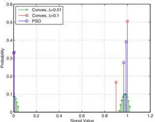
[0, 2] with a step size of Δ, and the results for Δ = 0.01 and Δ = 0.1 are considered. Fig. 1 illustrates the optimal probability distributions obtained from the PSO and the convex optimization algorithms.6It is calculated that the conventional algorithm, which uses a deterministic signal value of 0.8, has an average error probability of 0.3293, whereas the PSO
5For𝐾-dimensional vectors x and y, x ⪯ y means that the 𝑖th element ofx is smaller than or equal to the 𝑖th element of y for 𝑖 = 1, . . . , 𝐾.
6For the probability distributions obtained from the convex optimization algorithms, the signal values that have zero probability are not marked in the figures to clarify the illustrations.
0 0.2 0.4 0.6 0.8 1 1.2 0 0.1 0.2 0.3 0.4 0.5 0.6 Signal Value Probability Convex, Δ=0.01 Convex, Δ=0.1 PSO
Fig. 1. Probability mass functions (PMFs) of the PSO and the convex optimization algorithms for the noise PDF in (19).
and the convex optimization algorithms with Δ = 0.01 and Δ = 0.1 have average error probabilities of 0.2909, 0.2911 and0.2912, respectively. It is noted that the PSO algorithm achieves the lowest error probability with three mass points and the convex algorithms approximate the PSO solution with multiple mass points around those of the PSO solution. In addition, the calculations indicate that the optimal solutions achieve both the second and the fourth moment constraints in accordance with Proposition 4-b .
Next, the optimal signaling problem is studied in the presence of Gaussian mixture. The Gaussian mixture noise can be used to model the effects of co-channel interference, impulsive noise and multiuser interference in communications systems [5], [7]. In the simulations, the Gaussian mixture noise is specified by𝑝𝑁(𝑦) = ∑𝐿𝑙=1𝑣𝑙𝜓𝑙(𝑦 − 𝑦𝑙), where 𝜓𝑙(𝑦) =
e−𝑦2/(2𝜎2
𝑙)/(√2𝜋 𝜎𝑙) . In this case, 𝐺(𝑥) can be obtained from (9) as𝐺(𝑥) =∑𝐿𝑙=1𝑣𝑙𝑄 ((𝑥 + 𝑦𝑙)/𝜎𝑙). In all the scenarios,
the variance parameter for each mass point of the Gaussian mixture is set to𝜎2 (i.e.,𝜎2
𝑙 = 𝜎2 ∀𝑙), and the average power
constraint 𝐴 is set to 1. Note that the average power of the
noise can be calculated asE{𝑁2} = 𝜎2+∑𝐿
𝑙=1𝑣𝑙𝑦𝑙2. First,
we consider a symmetric Gaussian mixture noise which has its mass points at±[0.3 0.455 1.011] with corresponding weights
[0.1 0.317 0.083] in order to illustrate the improvements that can be obtained via stochastic signaling. In Fig. 2, the average error probabilities of various algorithms are plotted against
𝐴/𝜎2 when 𝜅 = 1.1 for both the sign detector and the
ML detector. For the sign detector, the decision rule at the receiver is specified by Γ0 = (−∞, 0] and Γ1 = [0, ∞). In this case, it is observed from Fig. 2 that the conventional algorithm, which uses a constant signal value of1, has a large error floor compared to the PSO and convex optimization algorithms at high 𝐴/𝜎2. Also, the average probability of error of the conventional signaling increases as𝐴/𝜎2increases after a certain value. This seemingly counterintuitive result is observed because the average probability of error is related to the area under the two shifted noise PDFs as in (5). Since the noise has a multi-modal PDF, that area is a non-monotonic function of 𝐴/𝜎2 and can increase in some cases as 𝐴/𝜎2 increases. It is also observed that the convex optimization algorithm performs very closely to the PSO algorithm for
0 10 20 30 40 50 10−4 10−3 10−2 10−1 100 10−5 A/σ2 (dB)
Average Probability of Error
PSO Convex, Δ=0.01 Convex, Δ=0.1 Conventional ML (Conventional) ML (Stochastic) Sign Detector
Fig. 2. Error probability versus𝐴/𝜎2for𝜅 = 1.1. A symmetric Gaussian mixture noise, which has its mass points at ±[0.3 0.455 1.011] with
corresponding weights[0.1 0.317 0.083], is considered.
densely spaced possible signal values, i.e., for Δ = 0.01. For the ML detector, the receiver compares𝑝𝑁(𝑦 −
√ 𝐴) and
𝑝𝑁(𝑦 +√𝐴), and decides symbol 0 if the latter is larger,
and decides 1 otherwise. It is observed for small 𝜎2 values that the ML receiver performs significantly better than the other receivers that are based on the sign detector. However, stochastic signaling causes the sign detector to perform better than the conventional ML receiver, which uses deterministic signaling, for medium 𝐴/𝜎2 values. For example, the PSO and convex optimization algorithms forΔ = 0.01 have better performance than the ML receiver for𝐴/𝜎2values from20 dB to40 dB. This is mainly due to the fact that the conventional ML detector uses deterministic signaling whereas the others employ stochastic signaling. However, when the stochastic signaling is applied to the ML detector as well, it achieves the lowest probabilities of error for all 𝐴/𝜎2 values as observed in Fig. 2 (labeled as “ML (Stochastic)”).
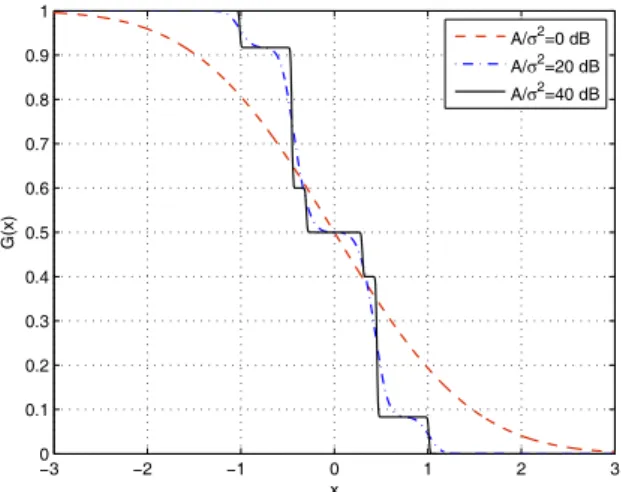
Another observation from Fig. 2 is that improvements over the conventional algorithm disappear as 𝜎2 increases (i.e., for small 𝐴/𝜎2 values). This result can be explained from Propositions 1 and 2, based on the plots of 𝐺(𝑥) at various 𝐴/𝜎2values. For example, Fig. 3 illustrates the plots of𝐺(𝑥) at𝐴/𝜎2of0, 20 and 40 dB for the sign detector. The function is decreasing and convex for 0 dB for the positive signal values, which are practically the domain of optimization since
𝐺(𝑥) is a decreasing function and the constraint functions 𝑥2
and𝑥4 are even functions.7 Therefore, Proposition 1 implies that the conventional algorithm that uses a constant signal value of1 is optimal in this case, as observed in Fig. 2. On the other hand, at20 dB and 40 dB, the calculations show that the condition in Proposition 2 is satisfied; hence, the conventional algorithm cannot be optimal in that case, and improvements are observed in Fig. 2 at 𝐴/𝜎2= 20 dB and 𝐴/𝜎2= 40 dB. Another result obtained from the numerical studies for Fig. 2 is that all the solutions achieve at least one of the second moment or the fourth moment constraints with equality as a result of Proposition 4.
7In other words, negative signal values are never selected for symbol 1 since selecting the absolute value of a negative signal value always gives a smaller average probability of error without changing the signal moments.
−3 −2 −1 0 1 2 3 0 0.1 0.2 0.3 0.4 0.5 0.6 0.7 0.8 0.9 1 x G(x) A/σ2=0 dB A/σ2=20 dB A/σ2=40 dB
Fig. 3. 𝐺(𝑥) in (9) for the sign detector in Fig. 2 at 𝐴/𝜎2values of0, 20 and40 dB. 0.5 0.6 0.7 0.8 0.9 1 1.1 1.2 0 0.1 0.2 0.3 0.4 0.5 0.6 0.7 0.8 Signal Value Probability Convex, Δ=0.01 Convex, Δ=0.1 PSO
Fig. 4. PMFs of the PSO and the convex optimization algorithms for the sign detector in Fig. 2 at𝐴/𝜎2= 20 dB.
For the scenario in Fig. 2, the probability distributions of the optimal signals for the sign detector are shown in Fig. 4 and Fig. 5 for𝐴/𝜎2 = 20 dB and 𝐴/𝜎2 = 40 dB, respectively, where both the PSO and the convex optimization algorithms are considered. In the first case, the convex optimization algorithm with Δ = 0.1 approximates the probability mass function (PMF) obtained from the PSO algorithm with two mass points (with nonzero probabilities), whereas the convex optimization algorithm withΔ = 0.01 results in 8 mass points. In the second case, the convex optimization algorithms with Δ = 0.1 and Δ = 0.01 result in PMFs with two and three mass points, respectively, as shown in Fig. 5. Since the convex optimization algorithm withΔ = 0.1 does not provide a PMF that is very close to those of the other algorithms in this case, the resulting error probability becomes significantly higher for that algorithm, as observed from Fig. 2 at𝐴/𝜎2= 40 dB.
Finally, a symmetric Gaussian mixture noise which has its mass points at±[0.19 0.39 0.83 1.03] each with a weight of
1/8 is considered. Such a noise PDF can be considered to model the effects of co-channel interference [7], or a system that operates under the effect of multiuser interference [5]. For
0.4 0.5 0.6 0.7 0.8 0.9 1 1.1 1.2 0 0.1 0.2 0.3 0.4 0.5 0.6 0.7 0.8 Signal Value Probability Convex, Δ=0.01 Convex, Δ=0.1 PSO
Fig. 5. PMFs of the PSO and the convex optimization algorithms for the sign detector in Fig. 2 at𝐴/𝜎2= 40 dB.
0 5 10 15 20 25 30 35 40 45 10−5 10−4 10−3 10−2 10−1 100 A/σ2 (dB)
Average Probability of Error
PSO Convex, Δ=0.01 Convex, Δ=0.1 Conventional ML (Conventional) ML (Stochastic) Sign Detector
Fig. 6. Error probability versus𝐴/𝜎2for𝜅 = 1.5. A symmetric Gaussian mixture noise, which has its mass points at±[0.19 0.39 0.83 1.03], each
with equal weight, is considered.
example, in the presence of multiple users, the noise can be modeled as𝑁 = ∑𝐾𝑘=2𝐴𝑘𝑏𝑘+ 𝜂, where 𝑏𝑘 ∈ {−1, 1} with
equal probabilities and 𝜂 is a zero-mean Gaussian thermal
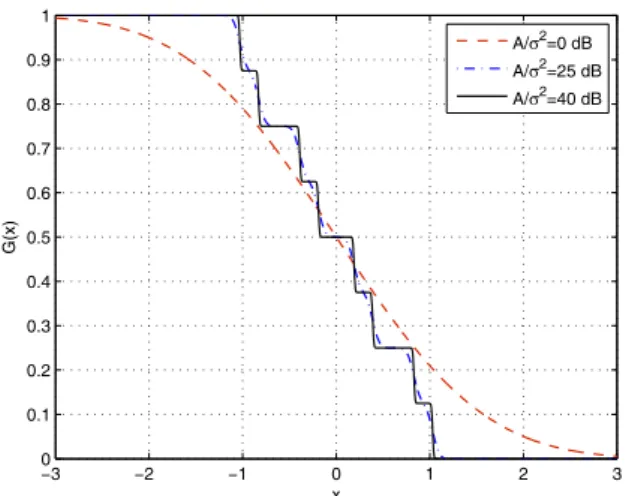
noise component with variance 𝜎2. Then, for 𝐾 = 4, 𝐴2 = 0.1, 𝐴3= 0.61 and 𝐴2 = 0.32, the noise becomes Gaussian mixture noise with8 mass points as specified at the beginning of the paragraph. In Fig. 6, the average error probabilities of various algorithms are plotted against the𝐴/𝜎2for𝜅 = 1.5 . Also the plots of𝐺(𝑥) at 𝐴/𝜎2= 0, 25, 40 dB are presented in Fig. 7, and the probability distributions at𝐴/𝜎2= 25 dB and
𝐴/𝜎2= 40 dB are illustrated in Fig. 8 and Fig. 9, respectively, for the sign detector. Although similar observations as in the previous scenario can be made, a number of differences are also noticed. The improvements achieved via the stochastic signaling over the conventional (deterministic) signaling are less than those observed in Fig. 2. In addition, since𝜅 = 1.5
in this scenario, only the second moment constraint is achieved with equality in all the solutions.
In order to investigate the optimal stochastic signaling for the ML detectors studied in Fig. 2 and Fig. 6, Table I presents
−3 −2 −1 0 1 2 3 0 0.1 0.2 0.3 0.4 0.5 0.6 0.7 0.8 0.9 1 x G(x) A/σ2=0 dB A/σ2=25 dB A/σ2=40 dB
Fig. 7. 𝐺(𝑥) in (9) for the sign detector in Fig. 6 at 𝐴/𝜎2values of0, 25 and40 dB. 0.4 0.5 0.6 0.7 0.8 0.9 1 1.1 1.2 0 0.1 0.2 0.3 0.4 0.5 0.6 0.7 0.8 0.9 Signal Value Probability Convex, Δ=0.01 Convex, Δ=0.1 PSO
Fig. 8. PMFs of the PSO and the convex optimization algorithms for the sign detector in Fig. 6 at𝐴/𝜎2= 25 dB.
the PDFs of the optimal stochastic signals in those scenarios, where the optimal PDFs are expressed in the form of𝑝𝑆(𝑥) =
𝜆1𝛿(𝑥 − 𝑥1) + 𝜆2𝛿(𝑥 − 𝑥2) + 𝜆3𝛿(𝑥 − 𝑥3). It is observed
from the table that the conventional deterministic signaling is optimal at low 𝐴/𝜎2 values, which can also be verified from Fig. 2 and Fig. 6 since there is no improvement via the stochastic signaling over the conventional one for those𝐴/𝜎2 values. However, as 𝐴/𝜎2 increases, the optimal signaling is achieved via randomization between two signal values. In those cases, significant improvements over the conventional signaling can be achieved as observed from Fig. 2 and Fig. 6. Finally, it is noted from the table that the optimal solutions result in randomization between at most two different signal levels in this example. This is in compliance with Proposition 3 since the proposition does not guarantee the existence of three different signal levels in general but states that an optimal signal can be represented by a randomization of at most three different signal levels.
0.4 0.5 0.6 0.7 0.8 0.9 1 1.1 1.2 0 0.1 0.2 0.3 0.4 0.5 0.6 0.7 0.8 0.9 Signal Value Probability Convex, Δ=0.01 Convex, Δ=0.1 PSO
Fig. 9. PMFs of the PSO and the convex optimization algorithms for the sign detector in Fig. 6 at𝐴/𝜎2= 40 dB.
TABLE I
OPTIMAL STOCHASTIC SIGNALS FOR THEMLDETECTORS INFIG. 2 (TOP BLOCK)ANDFIG. 6 (BOTTOM BLOCK).
𝐴/𝜎2(dB) 𝜆1 𝜆2 𝜆3 𝑥1 𝑥2 𝑥3 10 1 0 0 1 N/A N/A 15 1 0 0 1 N/A N/A 20 0.1181 0.8819 0 1.4211 0.9151 N/A 25 0.1264 0.8736 0 1.4494 0.8876 N/A 27.5 0.1317 0.8683 0 1.4465 0.8811 N/A 10 1 0 0 1 N/A N/A 15 1 0 0 1 N/A N/A 20 0.1272 0.8728 0 0.5073 1.0527 N/A 25 0.9791 0.0209 0 0.9950 1.2116 N/A 30 0.9415 0.0585 0 0.9859 1.2047 N/A 35 0.9236 0.0764 0 0.9823 1.1936 N/A
V. EXTENSIONS TO𝑀 -ARYPULSEAMPLITUDE
MODULATION(PAM)
The results in the study can be extended to 𝑀-ary PAM
communications systems for 𝑀 > 2 as well. To that aim,
consider a generic detector which chooses the 𝑖th symbol if
the observation is in decision regionΓ𝑖for𝑖 = 0, 1, . . . , 𝑀−1.
In other words, the decision rule is defined as
𝜙(𝑦) = 𝑖 , if 𝑦 ∈ Γ𝑖 , 𝑖 = 0, 1, . . . , 𝑀 − 1 . (27)
Then, the average probability of error for an 𝑀-ary system
can be expressed as Pavg=𝑀−1∑
𝑖=0
𝜋𝑖(1 − P𝑖(Γ𝑖)) , (28)
where𝜋𝑖 denotes the prior probability of the𝑖th symbol.
If signals𝑆0, 𝑆1, . . . , 𝑆𝑀−1 are modeled as stochastic
sig-nals with PDFs𝑝𝑆0, 𝑝𝑆1, . . . , 𝑝𝑆𝑀−1, respectively, the average probability of error in (28) can be expressed, similarly to (6), as Pstoc avg = 𝑀−1∑ 𝑖=0 𝜋𝑖 ( 1 − ∫ ∞ −∞𝑝𝑆𝑖(𝑡) ∫ Γ𝑖𝑝𝑁(𝑦 − 𝑡) 𝑑𝑦 𝑑𝑡 ) . (29) Then, the optimal stochastic signaling problem can be stated
as min 𝑝𝑆0,...,𝑝𝑆𝑀−1 𝑀−1∑ 𝑖=0 𝜋𝑖 ( 1 − ∫ ∞ −∞𝑝𝑆𝑖(𝑡) ∫ Γ𝑖𝑝𝑁(𝑦 − 𝑡) 𝑑𝑦 𝑑𝑡 ) subject to E{∣𝑆𝑖∣2} ≤ 𝐴 , E{∣𝑆𝑖∣4} ≤ 𝜅𝐴2 ,
𝑖 = 0, 1, . . . , 𝑀 − 1 . (30)
Due to the structure of the objective function in (30) and the individual constraints on each signal,𝑀 separate optimization
problems, similar to (8), can be obtained. Namely, for 𝑖 =
0, 1, . . . , 𝑀 − 1, min 𝑝𝑆𝑖 1 − ∫ ∞ −∞𝑝𝑆𝑖(𝑡) ∫ Γ𝑖𝑝𝑁(𝑦 − 𝑡) 𝑑𝑦 𝑑𝑡
subject to E{∣𝑆𝑖∣2} ≤ 𝐴 , E{∣𝑆𝑖∣4} ≤ 𝜅𝐴2 . (31)
In addition, if auxiliary functions 𝐺𝑖(𝑥) are defined as
𝐺𝑖(𝑥) ≜ 1 −∫Γ𝑖𝑝𝑁(𝑦 − 𝑥) 𝑑𝑦 for 𝑖 = 0, 1, . . . , 𝑀 − 1, the
optimization problem in (31) can be expressed as min
𝑝𝑆𝑖 E{𝐺𝑖(𝑆𝑖)}
subject to E{∣𝑆𝑖∣2} ≤ 𝐴 , E{∣𝑆𝑖∣4} ≤ 𝜅𝐴2 (32)
for𝑖 = 0, 1, . . . , 𝑀 − 1. Since (32) is in the same form as
(10), the results in Section III can be extended to𝑀-ary PAM
systems, as well.
VI. CONCLUDINGREMARKS ANDEXTENSIONS
In this paper, the stochastic signaling problem under second and fourth moment constraints has been studied for binary communications systems. It has been shown that, under cer-tain monotonicity and convexity conditions, the conventional signaling, which employs deterministic signals at the average power limit, is optimal. On the other hand, in some cases, a smaller average probability of error can be achieved by using a signal that is obtained by a randomization of multiple signal values. In addition, it has been shown that an optimal signal can be represented by a discrete random variable with at most three mass points, which simplifies the optimization problem for the optimal signal design considerably. Furthermore, it has been observed that the optimal signals achieve at least one of the second and fourth moment constraints in most practical scenarios. Finally, two techniques based on PSO and convex relaxation have been proposed to obtain the optimal signals, and simulation results have been presented.
In addition, the results in this paper can be extended to a generic binary hypothesis-testing problem in the Bayesian framework [2], [14].8 In that case, the average probability of error expression in (3) is generalized to the Bayes risk, defined as𝜋0[𝐶00P0(Γ0)+𝐶10P0(Γ1)]+𝜋1[𝐶01P1(Γ0)+𝐶11P1(Γ1)], where 𝐶𝑖𝑗 ≥ 0 represents the cost of deciding the 𝑖th
hypothesis when the𝑗th one is true. Then, all the results in
the paper are still valid when function𝐺 in (9) is replaced
by 𝐺(𝑥) = 𝐶01∫Γ0𝑝𝑁(𝑦 − 𝑥)𝑑𝑦 + 𝐶11∫Γ1𝑝𝑁(𝑦 − 𝑥)𝑑𝑦 .
Moreover, it can be shown that the results in this paper are also valid in the minimax and Neyman-Pearson frameworks [2] due to the decoupling of the optimization problem discussed in Section III.
8Hence, the results in the paper can be applied to other systems than communications, as well.
APPENDIX A. Derivation of (8)
The optimal stochastic signaling problem in (7) can be expressed from (6) as min 𝑝𝑆0,𝑝𝑆1 𝜋0 ∫ ∞ −∞𝑝𝑆0(𝑡) ∫ Γ1 𝑝𝑁(𝑦 − 𝑡) 𝑑𝑦 𝑑𝑡 + 𝜋1 ∫ ∞ −∞𝑝𝑆1(𝑡) ∫ Γ0 𝑝𝑁(𝑦 − 𝑡) 𝑑𝑦 𝑑𝑡 (33)
subject to E{∣𝑆0∣2} ≤ 𝐴 , E{∣𝑆0∣4} ≤ 𝜅𝐴2 (34) E{∣𝑆1∣2} ≤ 𝐴 , E{∣𝑆
1∣4} ≤ 𝜅𝐴2 (35)
For a given decision rule (detector) and a noise PDF, changing
𝑝𝑆0has no effect on the second term in (33) and the constraints
in (35). Similarly, changing𝑝𝑆1 has no effect on the first term
in (33) and the constraints in (34). Therefore, the problem of minimizing the expression in (33) over𝑝𝑆0 and𝑝𝑆1 under
the constraints in (34) and (35) is equivalent to minimizing the first term in (33) over 𝑝𝑆0 under the constraints in (34)
and minimizing the second term in (33) over 𝑝𝑆1 under the
constraints in (35). Therefore, the signal design problems for
𝑆0 and𝑆1 can be separated as in (8).□
B. Proof of Proposition 3
In order to prove Proposition 3, we take an approach similar to those in [11] and [29]. First, the following set is defined:
𝑈 ={(𝑢1, 𝑢2, 𝑢3) : 𝑢1= 𝐺(𝑥), 𝑢2= 𝑥2, 𝑢3= 𝑥4,
for∣𝑥∣ ≤ 𝛾}. (36)
Since 𝐺(𝑥) is continuous, the mapping from [−𝛾 , 𝛾 ] to ℝ3 defined by 𝐹 (𝑥) = (𝐺(𝑥), 𝑥2, 𝑥4) is continuous. Since the continuous image of a compact set is compact,𝑈 is a compact
set [30].
Let𝑉 represent the convex hull of 𝑈. Since 𝑈 is compact,
the convex hull 𝑉 of 𝑈 is closed [30]. Also, the dimension
of 𝑉 should be smaller than or equal to 3, since 𝑉 ⊆ ℝ3.
In addition, let 𝑊 be the set of all possible conditional
error probabilityP1(Γ0), second moment, and fourth moment triples; i.e., 𝑊 = { (𝑤1, 𝑤2, 𝑤3) : 𝑤1= ∫ ∞ −∞𝑝𝑆(𝑥)𝐺(𝑥)𝑑𝑥, 𝑤2= ∫ ∞ −∞𝑝𝑆(𝑥)𝑥 2𝑑𝑥, 𝑤 3= ∫ ∞ −∞𝑝𝑆(𝑥)𝑥 4𝑑𝑥, ∀ 𝑝𝑆(𝑥), ∣𝑥∣ ≤ 𝛾 } , (37)
where𝑝𝑆(𝑥) is the signal PDF.
Similarly to [29],𝑉 ⊆ 𝑊 can be proven as follows. Since 𝑉
is the convex hull of𝑈, each element of 𝑉 can be expressed
as v = ∑𝐿𝑖=1𝜆𝑖(𝐺(𝑥𝑖), 𝑥2𝑖, 𝑥4𝑖
)
, where ∑𝐿𝑖=1𝜆𝑖 = 1, and
𝜆𝑖≥ 0 ∀𝑖. Considering set 𝑊 , it has an element that is equal
tov for 𝑝𝑆(𝑥) =∑𝐿𝑖=1𝜆𝑖𝛿(𝑥 − 𝑥𝑖). Hence, each element of
𝑉 also exists in 𝑊 . On the other hand, since for any vector
random variable Θ that takes values in set Ω, its expected value E{Θ} is in the convex hull of Ω [11], it is concluded from (36) and (37) that𝑊 is in the convex hull 𝑉 of 𝑈; that
is,𝑉 ⊇ 𝑊 [31].
Since 𝑊 ⊇ 𝑉 and 𝑉 ⊇ 𝑊 , it is concluded that 𝑊 = 𝑉 .