Inferring phylogenetical tree by using hierarchical self organizing maps

(1)

INFERRING PHYLOGENETICAL TREE BY

USING HIERARCHICAL SELF ORGANIZING

MAPS

A THESIS

SUBMITTED TO THE DEPARTMENT OF COMPUTER

ENGINEERING

AND THE INSTITUTE OF ENGINEERING AND SCIENCE

OF BILKENT UNIVERSITY

IN PARTIAL FULFILLMENT OF THE REQUIREMENTS

FOR THE DEGREE OF

MASTER OF SCIENCE

By

Hayretdin Bahşi

January, 2002

(2)

I certify that I have read this thesis and that in my opinion it is fully adequate, in scope and in quality, as a thesis for the degree of Master of Science

Assist. Prof. Dr. Atilla Gürsoy (Supervisor)

Assist. Prof. Dr. Uğur Doğrusöz

Assoc. Prof. Dr. Volkan Atalay

Approved for the Institute of Engineering and Science

Prof. Dr. Mehmet Baray Director of the Institute of Engineering and Science

(3)

ABSTRACT

INFERRING PHYLOGENETICAL TREE BY USING

HIERARCHICAL SELF ORGANIZING MAPS

Hayretdin Bahşi

M.S in Computer Engineering

Supervisor: Assist. Prof. Dr. Atilla Gürsoy

Co-supervisor: Assist. Prof. Dr. Rengül Çetin Atalay

January, 2002

In biology, inferring phylogenetical tree is an attempt to describe the evolutionary history of today’s species with the aim of finding their common ancestors. Specifically in molecular biology, it is used in understanding the evolution relationships between proteins or DNA sequences. Inferring phylogenetical tree can be a very complicated task since even for the input data having thirty sequences, the best tree must be chosen among 1036 possible trees. In order to find the best one in a reasonable time, various hierarchical clustering techniques exist in the literature. On the other side, it is known that Self Organizing Maps (SOM) are very successful in mapping higher dimensional inputs to two dimensional output spaces (maps) without having any priori information about input patterns. In this study, SOM are used iteratively for tree inference. Two different algorithms are proposed. First one is hierarchical top-down SOM method which constructs the tree from the root to the leaves. Second one uses a bottom-up approach that infers the tree from the leaves to the root. The efficiency of Hierarchical SOM is tested in terms of tree topology. Hierarchical SOM gives better results than the most popular phylogeny methods, UPGMA and Neighbor-joining. Also this study covers possible solutions for branch length estimation problem.

(4)

HİYERARŞİK KENDİ KENDİNE ÖĞRENEN SİNİR

AĞLARIYLA FİLOGENETİK AĞAÇ YAPISININ

OLUŞTURULMASI

Hayretdin Bahşi

Bilgisayar Mühendisliği, Yüksek Lisans

Tez Yöneticileri: Yrd. Doç. Dr. Atilla Gürsoy,

Yrd. Doç. Dr. Rengül Çetin Atalay

Ocak, 2002

Biyoloji alanında filogenetik ağaç yapıları, şu anda varolan türlerin ortak atalarının belirlenerek bu türlerin evrimsel geçmişinin açıklanması amacıyla oluşturulur. Özellikle moleküler biyoloji alanında, bu ağaç yapıları, proteinlerin veya DNA dizilerinin evrimsel ilişkilerini ortaya çıkarmak için kullanılır. Çoğu zaman, filogenetik ağaç yapılarının oluşturulması zor ve karmaşık bir işlem gerektirmektedir. Örneğin, 30 DNA dizisine sahip bir girdi için 1036'dan fazla farklı ağaç yapısının arasından en iyisini seçmek gerekir. En iyi olan ağaç yapısının uygun bir zaman içinde belirlenebilmesi için literatürde bir çok hiyerarşik kümeleme teknikleri mevcuttur. Diğer yandan, kendi kendine öğrenen sinir ağları, girdi türleri hakkında her hangi bir bilgi sahibi olmadan çok boyutlu girdilerin iki boyutlu çıktı uzaylarına indirgenmesinde çok başarılı olmaktadır. Bu çalışmada, kendi kendine öğrenen sinir ağları yöntemi ard arda kullanılarak ağaç yapıları oluşturulmaktadır. Bu amaçla, iki farklı algoritma tasarlanmıştır. Birincisi, ağacı kökten başlayıp yapraklara doğru giderek oluşturmaktadır. İkincisi ise ağacı oluşturmaya yapraklardan başlamakta ve köke doğru ilerlemektedir. Tasarlanan algoritmalar ağaç topolojisinin doğruluğu göz önüne alınarak test edilmiştir. Bu algoritmalar, çok kullanılan UPGMA ve Komşu birleştirme metotlarından çok daha iyi sonuç vermektedir. Ayrıca bu çalışma, ağaç kollarının uzunluklarını tahmin etme problemi için de bazı çözümler sunmaktadır.

Anahtar Kelimeler: Filogenetik Ağaç Yapısı, Kendi Kendine Öğrenen Sinir Ağları, Evrim, DNA

(5)

ACKNOWLEDGEMENT

I would like to express my deep gratitude to my supervisor Dr. Atilla Gürsoy and my co-superviser Dr. Rengül Çetin Atalay for their guidance and suggestions throughout the development of this thesis.

I would like to thank Dr. Uğur Doğrusöz and Dr. Volkan Atalay for accepting to read and review this thesis.

I am grateful to my wife and my parents for supporting me during all the difficult times of my study.

(6)

List Of Figures

Figure 2-1. An example tree inferred from character data... 6

Figure 2-2. An example tree inferred from distance data ... 7

Figure 2-3. Inferred tree from ultrametric data ... 10

Figure 2-4. Inferred tree from additive data... 11

Figure 2-5. First step of tree inference with UPGMA... 14

Figure 2-6. Inferred tree after the second iteration of UPGMA... 15

Figure 2-7. Final inferred tree by UPGMA... 15

Figure 2-8. Final inferred tree by Neighbor-joining method ... 17

Figure 3-1. General structure of Self Organizing Maps... 20

Figure 3-2. An example SOM map produced ... 24

Figure 3-3. One cycle training of SOTA... 24

Figure 4-1. A sample transformation of character based input to numeric vector... 30

Figure 4-2. Classification of DNA sequences with SOM map ... 31

Figure 4-3. A sample trace of Hierarchic top-down SOM algorithm ... 34

Figure 4-4. A sample trace of Hierarchical Bottom-up SOM algorithm ... 37

Figure 4-5. The final tree inferred by Hierarchical Bottom-up SOM algorithm... 38

Figure 5-1. A sample phylogenetical tree ... 41

Figure 5-2. Phylogenetical tree of actin data inferred by Hieararchic Top-down SOM 43 Figure 5-3. Phylogenetical tree of actin data inferred by Neighbor-joining Method.... 43

Figure 5-4. Comparisons of test results according to topology testing method... 45

Figure 5-5. Efficiency of methods for different size input vectors ... 46

(9)

List of Tables

Table 2-1. A Sample for Binary Character State Matrix... 6

Table 2-2. Distance data matrix example... 7

Table 2-3. Ultrametric distance data ... 10

Table 2-4. Additive distance data... 11

Table 2-5 An example data matrix for UPGMA method... 13

Table 2-6. Data matrix at the end of first step of UPGMA... 14

Table 4-1. Transition probabilities according to Jukes-Cantor model ... 27

Table 4-2. A sample nucleotide distance matrix for Jukes-Cantor model ... 28

Table 4-3. Transition probabilities according to ... 28

Table 4-4. A sample nucleotide distance ... 29

Table 5-1. A sample distance data matrix ... 41

Table 5-2. Test results of all data sets according to topology testing method ... 44

Table 5-3. Test results of data sets having different sequence lengths ... 46

Table 5-4.Test results of Hierarchical bottom-up SOM for different initial learning rates ... 47

(10)

Chapter 1 1. Introduction

The dominant view about the evolution of life is that all the existing organisms are derived from common ancestors. New species are originated by splitting of common ancestors into two or more populations with slow transformations in a very long time. Therefore, evolution of life can be displayed by a tree which has a common root and all other nodes are its descendents. In literature, such trees are named as phylogenetical trees.

In biology, inferring phylogenetical tree is an attempt to describe the evolutionary history of today’s species, populations or other taxonomical units [2]. But specifically in molecular biology, phylogenetical tree is used in understanding the evolution relationships between proteins or DNA sequences. This study focuses on trees of DNA sequences.

A tree is that tree is an undirected acyclic connected graph [3] which is composed of exterior (leaves) and interior nodes. These nodes are connected to each other by edges. In phylogenetical tree, leaves are species or taxonomical units belonging to current time, interior nodes are ancestors of them and edges are the evolutionary distances between nodes. Evolutionary distances can be interpreted as the estimate of time that takes from evolution of one node from the ancestor node.

(11)

But generally this distance is not equivalent to elapsed time [2]. In a tree structure, there is only one path between each pair of nodes [3]. The evolutionary distance between any two nodes is the sum of edge lengths along this path.

Common problem of phylogenetical tree construction is determination of whether phylogenetical tree has root or not. In most of the phylogeny problems, determination of the root may not be available because of loss of data. In those cases, inferred trees will be unrooted.

Generally two main aspects of phylogenetical trees are important. First one is tree topology which is about how interior nodes are connected to leaves, and the second one is the amount of evolutionary distances assigned to edges between pairs of nodes.

There are two main types of input data for phylogenetical tree inferrence. One of them is the distance matrix data which has all the pair wise evolutionary distances of input sequences. The other one is the character state data matrix. In this matrix, there are discrete characters for each input sequence and each character may have different number of states. The aim in tree inferrence methods is finding the best tree fitting to this input data. But the inferrence method must select the appropriate tree among the huge number of possible ones. Even for 30 input sequences, the number of possible unrooted trees is nearly 1036. Searching all of the trees and finding the best one is an option, but it is impossible to reach the solution in a reasonable time for data-sets having more than 20 sequences. In order to overcome this difficulty, two main categories of inferring tree methods are decided. First category includes clustering methods which use distance matrix data. These methods directly calculates the optimum tree from the input data. But generally the inferred tree is not the best one. The second type of methods use two major steps. First step is determination of an optimality criteria (objective function) for evaluating the given tree. The second step is computing the value of objective function with specific algorithms and finding the best trees according to this criterion. The second method is usually slower than the first one but yields better results.

This study tries to improve the performance of distance based methods in terms of tree quality by using self organizing map which is a type of neural network. SOM

(12)

(Self Organizing Map) uses unsupervised learning method. It is a very powerful clustering method and used in many areas of computational biology. Its strength comes from having the ability of detecting second and higher order correlations in patterns [8]. It can succesfully map high dimensional inputs to two dimensional output spaces which are generally maps having predefined sizes. In inferring phylogenetical tree problem, two main issues effect the quality of tree: Tree topology and edge lengths which constitute evolutionary distances. If SOM is used in this problem, it can give better quality tree topologies with the help of its clustering strength. Since tree inference is not a simple clustering problem, SOM must be used hierarchically.

In literature, there are some studies which use SOM in clustering proteins or DNA sequences [8,13]. In these studies, SOM is just used only for clustering and visualization purposes. SOM is also used for inferrence of phylogenetical tree (SOTA [9]). But this study is not very sufficient in terms of proving the quality of its' results.

In this study, two different algorithms are constructed by using SOM hierarchically. First one is the top-down approach which constructs the tree starting from the root to the leaves and the second one is a bottom-up approach which infers the tree from the leaves to the root. These methods propose solutions for determination of tree topology.

In order to prove quality of inferred trees in terms of tree topology, a test method is proposed. This method considers that all the edge lengths are unit distances. It evaluates the inferred tree according to the distance matrix. Test results are compared with the results of Neighbor-joining and UPGMA methods which are the most famous distance based methods. Hierarchical SOM algorithms give better results than Neighbor-joining and UPGMA algorithms. Then, the performance of hieararchic SOM is fine tuned with adjusting the SOM parameters.

It is known that accurate estimation of branch lengths is the another important factor in the quality of phylogenetical tree. This study also covers three different intuitive solutions for this problem, average, weight and consensus vector methods. These methods are compared with the results of Neighbor-joining and UPGMA by using a method which estimates the error of inferred tree in terms of branch lengths.

(13)

But Neighbor-joining and UPGMA are better according to test results. More efforts are needed for adaptation of Hierarchical SOM algorithm to branch length estimation problem.

The following section, Chapter 2, provides detailed background information about different phylogenetical tree inferrence methods that exist in literature. Chapter 3 focuses on SOM itself with SOM usage in protein clustering and inferring phylogenetical tree problems. Chapter 4 gives details of Hierarchical SOM algorithms. Then Chapter 5 presents tree topology testing method and discussion of Hierarchical SOM test results. Chapter 6 describes some studies which are presented for branch length estimation problem. Last chapter, Chapter 7 concludes overall study.

(14)

Chapter 2 2. Background on Phylogenetical Tree

This chapter includes an overview of phylogenetical tree inference methods. In first part of this chapter, general information will be given about input data types for this problem. This information is important because tree inference methods basically differ in terms of input data. In other words, input data types show the logics under the methods. After presentation of input data types, categories of tree inference methods will be described.

2.1 Input Data Types

Input data types can be classified into two main categories as character based and distance based data.

2.1.1 Character-Based Data

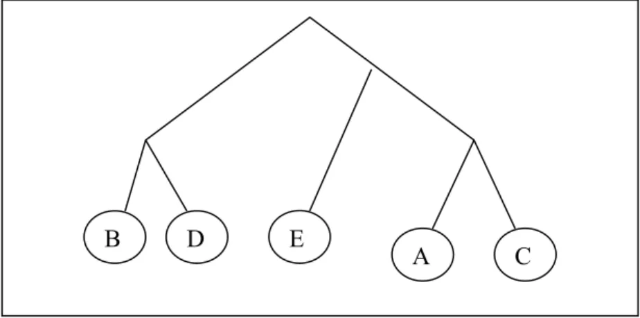
In this data type, each input objects (DNA sequences or proteins) have discrete characters and each of the characters have a finite number of various states. The data relative to these characters are placed in an objects * characters matrix, which we call character state matrix. For example, in Table 2-1, there exists an example character state matrix showing that whether each of five different objects A,B,C,D,E have the properties C1, C2, C3, C4 and C5 or not. In this matrix, '0' means that corresponding property does not exist in associated object. '1' says object has that property. If Table

(15)

2-1 is observed carefully, it can be said that protein A has c3 and c4 properties but has no others, protein B has c1 and c2 properties etc… The tree in Figure 2-1 is constructed from the character state matrix in Table 2-1 (Details about creation of tree from the given data is not important now).

In the inferred tree, similar objects are located in closer nodes. For example, objects 'B' and 'D' have four common properties which mean they are highly similar to each other. This similarity is reflected to tree topology so that they are sister nodes. Since 'E' has different characters from B or D, they belong to disjoint sub-trees.

Figure 2-1. An example tree inferred from character data

Number of character states may change in various problems. For a sequence, number of character states is 4 (A,T,G,C) for DNA and 21 for amino acids.

Objects C1 C2 C3 C4 C5 A 0 0 0 1 1 B 1 1 0 0 0 C 0 0 0 1 0 D 1 1 1 0 0 E 0 0 1 0 1

Table 2-1. A Sample for Binary Character State Matrix

E

A C

(16)

2.1.2 Distance-Based Data

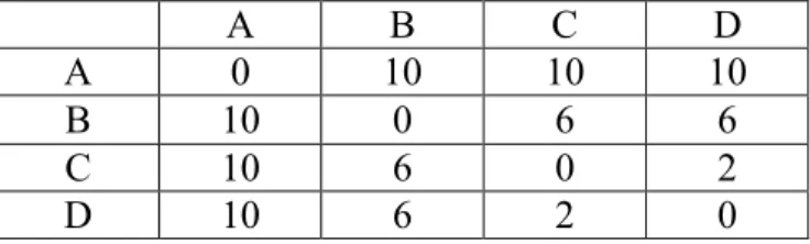
In this type of data, source of information is a square matrix which has the evolutionary distances between all pairs of input objects. This matrix is known as distance matrix. There is an example distance matrix shown in Table 2-2. Each numeric value is evolutionary distance between corresponding objects.

Reflection of this matrix to a phylogenetical tree is in Figure 2-2. After the construction of phylogenetical tree according to distance matrix, it can be seen that objects having less distances are closer to each other in the tree. In matrix, 'A' is the most distant object from the others and this can be also seen in the inferred tree. Objects 'C' and 'D' are the closest pair in matrix and it is exactly reflected to the tree.

Figure 2-2. An example tree inferred from distance data

A B C D

A 0 10 10 10

B 10 0 6 6

C 10 6 0 2

D 10 6 2 0

Table 2-2. Distance data matrix example

1 1 2 3 2 5 A B C D

(17)

2.2 Methods of Inferring Phylogenetical Tree

Phylogenetical tree inference methods must overcome big difficulty, lack of enough data about history. It predicts the historical ancestors of today's species, but generally we don't have direct information about past [2]. Source information is generally existing molecules or species. So, tree prediction is done by elimination of tree candidates among the all possible trees with the limited knowledge and finding the best one. The first solution that may come to mind can be exhaustive searching of all possible trees. But two big problems arise at this stage. One of them is the huge amount of possible tree combinations for even small number of input sequences. For example, if there exist 10 input sequences, the number of possible trees exceeds two million. For data sets having more than 20 sequences, finding the best tree in a reasonable time is impossible. The second and more serious problem is how it can be determined that whether one tree is better than the other. So, tree inference solutions firstly need to present an optimality criterion (objective function) for the evaluation of any given tree. The result of this evaluation is used to compare any tree with the others. Then, the solution needs an algorithm for finding the best tree according to this objective function. It must be pointed out that objective function is not used for only evaluation of a tree. More or less (according to quality of objective function) it may help to shrink the possible tree search space. So, some heuristic algorithms can be used from that point. But, there exist another approach which combines the objective function and best tree finding method into one complete algorithm. Rather than solving the problem in two steps, it tries to reach to solution with just one step. Hierarchical clustering techniques are widely used for this aim. This approach is faster than the first one but tree quality can be lower. On the other side, first solution can still suffer from reaching to the best tree in a reasonable time.

In the lights of previous descriptions, inferring tree algorithms can be categorized into two broad types: Distance based methods and maximum-parsimony methods. Distance-based methods use the input data which is the pair wise evolutionary distances of all input sequences. The main goal is reflecting all these distances correctly to a tree. These methods combine objective function and optimal tree finding algorithm

(18)

into one complete solution by using clustering techniques. On the other side, maximum-pasimony methods take the approach of two steps solution. They do not reduce biological datum to evolutionary distances, they use character-based data directly [7]. The goal is building a tree structure in which input sequences are put to the leaves of the tree and sequences of ancestor nodes are inferred so that the mutations implied in the evaluation history is minimized. Objective function must be chosen in order to minimize the mutations [2]. In the following two sections, more detailed information about these methods will be given.

2.2.1 Distance-based Methods

Main differences of these methods with the others are that they use distance-based data. These methods consider the problem in such a way that input sequences are points in a euclidean vector space and all the pair wise distances between these points are known. From that point, phylogeny problem is transformed into a clustering problem. But in order to construct the tree structure, recursive clustering techniques are used.

Basically, quality of inferred tree is related with two main issues in these types of methods. First one is tree topology which is about how leaves are connected to interior nodes. The second one is the quality of branch length estimations. So tree inference methods must provide efficient solutions for both of these problems in order to produce better results [2].

The properties of inferred trees are another important topics for distance-based methods. Because final structural properties like being rooted or unrooted, are closely related with these properties. There are two main types of tree properties, ultrametric and additive property.

• Ultrametric Property

A tree has ultrametric property if the distances between any pairs of sequences are equal to the total length of branches joining them and all of the sequences have the same evolutionary distances from the root node.

(19)

Formal definition of ultrametric property is as follows:

Let D is the distance data matrix of sequence set and T is the rooted tree where the leaves of the tree correspond to sequences. This tree is ultrametric if the following conditions:

1. Each internal node of the tree is labeled by one distance from data matrix. 2. While going down from the root to leaves, the labeling numbering decreases. 3. For any sequence pair (i,j), D(i,j) is the label of least common ancestor of

sequences i and j. [1]

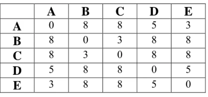
Suppose that there is a symmetric distance data matrix as shown in Table 2-3

A B C D E

A

0 8 8 5 3

B

8 0 3 8 8

C

8 3 0 8 8

D

5 8 8 0 5

E

3 8 8 5 0

Table 2-3. Ultrametric distance data

Tree (in Figure 2-3) can be inferred from this data as definition describes. It can be realized that tree exactly reflects the input data matrix and each leaves have equal distance from the root node.

Figure 2-3. Inferred tree from ultrametric data 3 3 5 8 A E D B C

(20)

The key point of ultrametric property is that if an ultrametric tree can be constructed from the given data, it means this tree is a perfect rooted phylogeny tree. In other words, tree can be a rooted tree if it is ultrametric.

• Additive Property

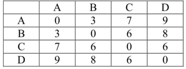
A tree has additive property if the distances between any pairs of sequences are equal to the total lengths of branches joining them.

Formal definition is as follows:

Let D is the symmetric distance data matrix for n sequences. Let T is the edge weighted tree with n leaves. Tree T is called an additive tree for the given data matrix if the distances between every pair of leaves in the tree are the same as in the matrix data [1]. Suppose that there is a matrix data as shown in Table 2-4.

A B C D A 0 3 7 9 B 3 0 6 8 C 7 6 0 6 D 9 8 6 0 Table 2-4. Additive distance data

A tree can be inferred from this data as in Figure 2-4. All the distances in the tree are consistent with the matrix data. So it is additive tree.

Figure 2-4. Inferred tree from additive data

If the phylogeny tree has the additive property, it is a perfect unrooted tree. But ultrametric property is stronger because it can lead to a rooted tree.

2 4 3 1 2 A B C D

(21)

According to these tree properties, distance-based methods can be categorized. Two different distance-based methods exist; UPGMA (or WPGMA) and neighbor- joining.

2.2.1.1 UPGMA(Unweighted Pair Group Method) and WPGMA (Weighted Pair Group Method)

These are algorithms for inferring trees from ultrametric distance data. If data is not ultrametric , data can not fit to a perfect tree and some errors will be occurred [2]. The general descriptions of these algorithms are as follows:

Input data is distance matrix of sequences. Let dij is the distance between

sequence ‘i’ and sequences ‘j’. First step is finding the pair of sequences with the smallest distance. Then, these sequences are combined and they form a single new sequence from that time. The distances of this new sequence (actually it is a cluster of sequences) to others are calculated and they are added to data matrix. Also distance data of old ones are erased Then again pair of sequences those having minimum distance will be found. These merging processes continue until there remains one cluster including all sequences. The steps of algorithm are as follows:

1. Each sequence is considered as a unique cluster.

2. From the distance matrix, find the clusters i and j such that dij is the

minimum value

3. Length of branch between i and j will be dij /2

4. If i and j were the last clusters then tree is completed otherwise create a new cluster called u.

5. Distance from u to each other cluster k (k≠i or j) is the average value of

dki and dkj

6. Eliminate clusters i and j, add cluster u and return to step 2

Outline of clustering method is described above. But variations of these methods can be implemented by changing the average function of step 5. The mostly common used

(22)

average function is the function which UPGMA algorithm uses. In this method, average is calculated according to the number of sequences in the cluster. Suppose that cluster i contains Ti sequences and cluster j contains Tj sequences. After merging of these two

clusters, new cluster u is created and distance between cluster u and any other cluster k is calculated with Expression 2.1.

dku = (Ti dki + Tj dkj )/ (Ti + Tj ) (2.1)

At the averaging step, WPGMA (weighted pair group method) uses simple averaging function (2.2).

dku = (dki + dkj )/ 2 (2.2)

Average function can be maximum (2.3) or minimum (2.4) value of two distances

dku = max(dki ,dkj ) (2.3)

dku = min(dki ,dkj ) (F6) (2.4)

If input data for clustering method is ultrametric, all of average functions infer the same tree.

There is a sample of sequence data matrix in Table 2-5. This matrix includes the distances of 5 rRNA sequences, Bsu, Bst, Lvi, Amo and Mlu.

Bsu Bst Lvi Amo Mlu

Bsu 0 0.1715 0.2147 0.3091 0.2326

Bst 0 0.2991 0.3399 0.2058

Lvi 0 0.2795 0.3943

Amo 0 0.4289

Mlu 0

(23)

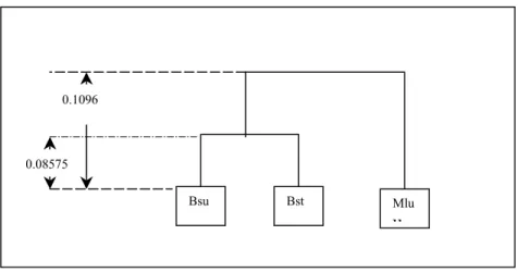
Let’s apply the UPGMA method to above data. At the first step, it can be realized that the minimum distance is between Bsu and Bst. Then, these sequences form one cluster. Inferring of tree is started as shown in Figure 2-5. Length of branch is calculated with dividing the distance between Bsu and Bst by two. ( 0.1715/2=0.08575)

Figure 2-5. First step of tree inference with UPGMA

The next step is calculating the new data matrix. The new data matrix is in Table 2-6. Distances between Bsu-Bst and other sequences are calculated with the Expression 2.1.

Table 2-6. Data matrix at the end of first step of UPGMA

The second clustering iteration again starts with finding the smallest distance which is between Mlu and Bsu-Bst. At the end of this iteration, inferred tree is in Figure 2-6. After all iterations, tree is completed. The complete tree is shown in Figure 2-7.

Bsu-Bst Lvi Amo Mlu

Bsu-Bst 0 0.2569 0.3245 0.2192 Lvi 0 0.3399 0.3943 Amo 0 0.4289 Mlu 0 0.08575 0.08575 Bsu Bst

(24)

Figure 2-6. Inferred tree after the second iteration of UPGMA

Figure 2-7. Final inferred tree by UPGMA

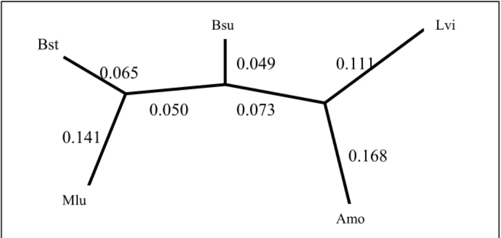
2.2.1.2 Neighbor-Joining Method

This method infers additive tree. It uses basic clustering methodology of UPGMA algorithm. The difference occurs in choosing of the clusters for the merging process. Neighbor-joining does not only join the closest clusters, it combines the clusters which are far from the rest. This method uses the minimum-evolution criteria that can be calculated by Expression 2.5 [12].

0.08575

Bsu Bst Mlu

u 0.1096

Bsu Bst Mlu Amo Lvi

0.08575 0.1096

0.1398 0.1655

(25)

distij =Dij - ui – uj (2.5)

distij : minimum evolution distance between sequence i and j

ui : distance of sequence i to the rest of sequences

ui = ∑k≠i Dik /(n-1) (2.6)

UPGMA uses directly the distance matrix data for the merging process. But Neighbor-joining method computes a new data matrix by using minimum evaluation criteria. Firstly, average distance of each cluster to other clusters are computed by Expression 2.6. Then for all pairs, minimum evolution distance is calculated by Expression 2.5 and new data matrix is formed with these values. Selecting the appropriate clusters for the merging process is done according to this data matrix.

General outline of this algorithm is as follows:

1. Each sequence is considered as a unique cluster. 2. For each cluster i compute ui by Expression 2.6.

3. Compute the whole minimum evaluation distance matrix by expression 2.5.

4. Choose the minimum distij value from the minimum evaluation distance

matrix.

5. Join i and j, and define new cluster named w.

a. Calculate the branch lengths from i and j to the new node w as

diw = ½ Dij + ½ (ui - uj ), djw = ½ Dij + ½ (uj – ui )

b. Compute the new distances between cluster w and other clusters by the following formula:

Dwk = (Dik + Djk - Dij )/2

6. Delete the sequences i and j from matrix and enter the new one, w. 7. If more than two clusters still exist return to step 2, otherwise merge two

(26)

Inferred tree with Neighbor-joining method for the example data set in Table 2-5 is shown in Figure 2-8.

Figure 2-8. Final inferred tree by Neighbor-joining method 2.2.2 Maximum-Parsimony Methods

In science, parsimony means that simpler hypotheses are preferable to more complicated ones. In computational biology, it is the name of mostly used method for inferring tree from character-based data. These methods solve the tree inference problem in two distinct steps. First step is defining an optimality criterion (objective function) to compare different possible trees. The next step is finding trees those best matches to the optimality criterion [2].

The main aim is finding the tree with the shortest total length. In these methods, unit of length is evolutionary steps occurring during the transformation of one character state to another. Steps can be base substitutions for nucleotide sequence data or gain, loss events for restriction site data. There exist a common objective function for the evaluation of any given tree. This function calculates total number of character state changes along the all branches in the tree. In order to calculate total character state changes, it traverses all branches of tree and assigns a cost value to each of them. Here, cost is actually the number of character state changes that occurs along the tree branch. Sum of all branch costs is total character changes. Optimal tree searching algorithms evaluates all possible trees and finds the best tree with the minimal character changes.

0.073 0.050 0.168 0.111 0.049 0.065 0.141 Bst Bsu Lvi Amo Mlu

(27)

2.2.3 Optimal Tree Searching Algorithms

Determining the optimal tree criterion and evaluating the existing tree structure according to this criterion are different problems as stated before. Clustering algorithms like UPGMA and Neighbor-joining methods solve the problem without determining optimal tree criterion. The algorithms stated in this category solve the problem of finding tree topology and predicting tree branch lengths according to the predetermined criterion. They are mostly used with maximum-parsimony methods.

Finding the optimal tree is very expensive task in terms of needed computational power because there exists huge number of possible trees even for small number of inputs.

(28)

Chapter 3 3. Background on Self Organizing Maps and

Their Application to Phylogeny Problem

This chapter gives general information about SOM algorithm and introduces some phylogeny studies with SOM.

3.1 Overview of SOM Algorithm

Self Organizing Map [6] is a neural network type which uses unsupervised learning method. Neural networks is very promising tool for application to many areas of biology. They are able to detect second and higher order correlations in inputs [8]. They generate a mapping from high dimensional input space to lower dimensional output usually to two dimensional systems which are called SOM maps. It reflects the actual correlations of inputs to the map. Also training of this system does not need to have a previous knowledge about the inputs.

3.1.1 SOM Map

Basically, SOM map is an array of interconnected neurons (cells) as in Figure 3-1. All cells in the input layer are connected to all cells in output layer. The spatial location of

(29)

a cell in the map corresponds to a specific region of the input space. Main aim is providing that nearby inputs are categorized in the nearby map locations. In order to supply this correlation between input space and output space, map is trained with a training data set. For training, unsupervised competitive learning algorithm is used.

Figure 3-1. General structure of Self Organizing Maps

Each cell has a weight (reference) vector which is formed through the training process. For each input, the euclidean distances between the weight vectors of each cell and the input vector are calculated. The cell with the closest match of the input and its weight vector produces an active output. In other words, each cell behaves like a pattern detector for the same input and winning cell of the competition is the pattern that most resembles to the input.

3.1.2 Unsupervised Learning

Formation of the weight vectors of cells occur through a training process. Generally, training is done with a distinct training data set. Weight vectors are initialized by random values or by input vectors drawn randomly from training data. Each input from this set is presented to SOM system in order to calculate weight

Input Layer

Input

(30)

vectors. Winning cell for the each input is found. Then some of the cells are adapted according to the input. Amount of adaptation and determination of cells that will be adapted are the most important points of learning phase. Because these issues produce the topological characteristic of the map. For example if only the weight vector of the winning node is adapted, similar inputs are not placed in closer cells. In other words, neighborhood property disappears. If all weight vectors are equally adapted, SOM map could not accurately cluster the inputs. Special function which is known as neighborhood function is used for choosing the cells which needs to adaptation. And another function, learning rate function adjusts the amount of adaptation.

3.1.3 Neighborhood and Learning Rate Functions

According to neighborhood function, maximum adaptation will occur at the winning node and neighborhood nodes of winning node are also updated. It has been found experimentally that in order to achieve global ordering of the map, the neighbourhood function firstly covers all of the cells to quickly produce a rough mapping, but then it is reduced with time (here time means number of passes through the training set data) to supply more localized adaptation of the map. Learning rate is another factor in learning process which decreases with time. In order to achieve quicker convergence of the algorithm, initially the learning rate should be high to produce coarse clustering of nodes. As time passed, adaptation rate makes smaller changes to weight vectors and local properties to the map are given.

Suppose that we want to train a SOM map which has K number of cells with input vectors set {x | x∈Rn}(n is the vector size). Each cell has a weight vector wk

(k=1,....,K). t is the time index and x(t) represents the input that is presented to SOM system at time ’and wk(t) is the weight vector computed at time t.

The differences between input vector and weight vector is calculated with Euclidean distance method for all weight vectors

dk(t) =|| x(t) - wk(t) ||, (k=1,...K) (3.1)

(31)

dc(t) = min dk(t) (3.2)

(k=1,...,K)

After determination of winning node, weight vectors are updated according to the following formula:

wk(t+1) = wk(t) + α(t) hck (t) (x(t) - wk(t)) (3.3)

In this function α(t) is the learning rate function and hck (t) is the neighborhood function.

Its' exact form is not important and can be linear, exponential or inversely proportional to time. The following function can be used for adjusting the learning rate:

α(t) = α0.(1-t/ ttotal) (3.4)

Here, ttotal is the time of whole training process. At t=0, this function is equal to an

initial predetermined value which is α0. As time increases it monotonically decreases.

Basically, two neighborhood functions may be used. First one is the Expression 3.5. In this expression, rk and rc denote the coordinates of cell k and winning cell c,

respectively. σ(t) determines the width of the neighborhood function which decreases during training from initial value that is dimension of lattice to last value of dimension of one cell.

hck (t) = exp (-|| rk - rc ||2 / σ(t)2) (3.5)

A variety of neighborhood functions can be used. The neighborhood function can also be constant around the winning cell. Instead of Expression 3.5, the simpler function in Expression 3.6 can be used.

hck (t) =

[

(3.6)

1 if || rk - rc || <= σ(t)

(32)

3.2 Phylogeny Solutions with SOM

Several studies have been made for different purposes in sequence analysis by using neural network methods. Especially, they are used to classify biological sequences but these neural network methods are based on supervised learning [15]. So in these methods the classification knowledge of training set must be given which is difficult to determine in large set of data. But in unsupervised methods, this priori information is not needed and method itself categorizes the data. These methods can fit to the needs of sequence analysis problem. Unsupervised neural network algorithms are used in some studies for classification of protein sequences [8,13]. In these studies, proteins are simply categorized with a predetermined size of SOM map. SOM is used in the field of inferring phylogenetical tree by the study, named SOTA [9].

In SOM algorithm, map that is used for classification of data has certain topology which is generally a grid like structure with two dimensions. But this structure does not easily fit to a tree structure. SOTA solves this problem by using growing cell structures algorithm of Fritzke [10] and a tree like structure for the map. Growing cell structures algorithm simply divides the parts of map into much more components if the number of inputs belonging that parts are bigger. An example is shown in Figure 3-2. Suppose that we run SOM algorithm and get the distribution of inputs in SOM map as in the left of the figure. Part a has much more elements so it is needed to divide into much more components. At the next step that part is divided as shown in the figure. Since other parts b, c and d have small number of inputs, they aren't needed to be divided. SOTA combines this growing structure decision with tree-like structured map. Initial structure is composed of one root and two terminal nodes. Each terminal node behaves like a cell and has unique weight vector which is randomly initialized. Each node also has a variable called local resource. It handles the heterogeneity of inputs belonging to that node. If one input is assigned to a winning cell, the distance between that input and weight vector is added to this variable. If a cell reaches to a heterogeneity value more than the threshold, is divided into two descendent cells.

(33)

Figure 3-2. An example SOM map produced

by growing cell structures algorithm

Figure 3-3. One cycle training of SOTA

Suppose that we have five sequences as in Figure 3-3. Initial map is composed of one root and two terminal nodes. During the training, winning node for sequences 1,3 and

4 is C1, and winning node for sequence 2 and 5 is C2. After determination of winning

nodes of each input, weight vector of corresponding node is updated as usual. But the local resource variable is also computed. Consider the local resource variable of C1

a b c d Root C1 C2 seq1 seq2 seq3 seq4 seq5 Root C1 C2

Initial structure _seq1

seq3 seq4 seq2 seq5 one cycle training

Sequences are categorized according to winning nodes

(34)

exceeds the threshold. Then two children of this node are created. At the end of the training the whole tree structure is constructed and all weight vectors of nodes are determined. This tree like map can be used for the categorization of inputs.

Since learning is adapted to tree structure directly, SOTA has problems with the neighborhood condition. Global arrangements are done at the first stages in small neighborhood area, some errors in these arrangements lead to totally wrong trees at the end. This study doesn't provide comparative experimental results of real world data with other methods to prove the efficiency of algorithm.

(35)

Chapter 4 4. Hierarchical SOM Algorithms

We proposed a new algorithm for inferring phylogenetical trees based on hierarchical SOM maps. The first aim is adapting the conventional SOM approach to inferring phylogenetical tree problem without destroying neighborhood and unsupervised learning properties of SOM. Since output of SOM is a two dimensional map, in this algorithm SOM maps are used hierarchically [18] in order to produce tree structure. Input data for this algorithm is character-based data but it is converted to numerical input vectors. Euclidean distances between these vectors are used in the clustering process. So, it is an alternative method for distance-based methods presented in Chapter 2.

Two different approaches of Hierarchical SOM method are presented in this study. One of them uses top-down approach that constructs the tree from the root to the leaves and the second one uses bottom-up approach that forms the tree in opposite direction, from the leaves to the root. The details will be covered in the related sections. In this chapter, firstly, transformation of character-based data to numerical vectors is

(36)

described. Then, detail of the SOM clustering technique is given. Finally, the hierarchical SOM approach is presented.

4.1 Transformation of Character Data to Numeric Vectors

DNA sequences are composed of four alphabet letters A, G, C, T and in biology each of them is named as nucleotide. We want to represent each DNA sequence with a vector such that Euclidean distance between the vectors of two DNA sequences are proportional to their relativeness. First of all, the distances between each nucleotide must be determined. To determine distances, help of nucleotide substitution models is needed. Because, substitution rates between nucleotides may represent the similarities between each other and these similarity definitions can be transformed into distance values between sequences.

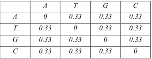
Substitution models define how and in which rate nucleotide substitutions (mutations) may occur during the evolution. Jukes-Cantor model is the simplest one and assumes that there is independent change at all sites (characters) with equal probability [2]. According to this definition, substitution probabilities of nucleotides can be represented as in Table 4-1 (a is probability value where 0<3a<1 ).

A T G C A 1-3a a a a T a 1-3a a a

G a a 1-3a a

C a a a 1-3a

Table 4-1. Transition probabilities according to Jukes-Cantor model

Substitution rates can be considered as a similarity metric because a correlation between similarity and substitution rates can be found [17]. Also it must be noted that similarity and distance is the two side of one reality. Maximization of similarity is the minimization of distance. So higher substitution rates are the evidences of lower distances. Since in Jukes-Cantor model, all substitution rates are equal, the distances

(37)

between different nucleotides can also be considered as equal. So, matrix that is given in Table 4.2 can be the distance matrix of nucleotides under Jukes-Cantor model.

Table 4-2. A sample nucleotide distance matrix for Jukes-Cantor model

Nucleotide bases fall into two categories depending on the ring structure of the base. Purines (Adenine and Guanine) are two ring bases, pyrimidines (Cytosine and Thymine) are single ring bases. A mutation that preserves the ring number is called a transition (A <-> G or C <-> T ), a mutation that changes the ring number is called transversion which occur between a purin and a pyrimidine (e.g. A <-> C or A <-> T). The number of transitions observed in nature is much greater than the number of transversions.

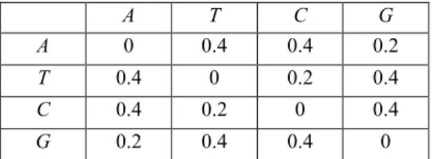
There is another substitution model called Kimura-2-parameter model [2]. This is more complicated so that two different substitution rate values are used in this model. Kimura-2-parameter model takes these transition and transversion rates into consideration and presents a substitution model that is specified in Table 4-3.

A T C G A 1-a-2b b b a T b 1-a-2b a b C b a 1-a-2b b G a b b 1-a-2b

Table 4-3. Transition probabilities according to

Kimura-2-Parameter model

In this Table a represents the transition rate and b is the transversion rate. It is known that transition rates are bigger than transversion rates. Since higher substitution rates

A T G C A 0 0.33 0.33 0.33 T 0.33 0 0.33 0.33 G 0.33 0.33 0 0.33 C 0.33 0.33 0.33 0

(38)

mean lower distances, data matrix given in Table 4-4 can reflect the distances between nucleotides according to the Kimura-2-Parameter model.

Table 4-4. A sample nucleotide distance matrix for Kimura-2-Parameter Model

In this study, Table 4.4 is used as a nucleotide distance matrix.

After determination of nucleotide distance matrix, it is time to convert the character data to numerical vectors. Firstly all input sequences must be aligned. Then, for each nucleotide in the DNA sequence, all four values along the corresponding row of the nucleotide distance matrix are appended to input vector. It is clear that one numerical value can not be used for each nucleotide because each nucleotide has different distances to others and these distance information must be given to each vector. Figure 4-1 shows an example for generation of numerical input vectors. The sequence AGTA is given to vector creation machine, appropriate values according to Table 4-4 are appended to result vector for each letter.

Sometimes, information about some nucleotide positions can be lost due to a reason. In DNA sequences, those positions are considered as gaps and they are shown by character ‘-‘. Also gaps may be inserted to sequences by alignment methods. Logically, gaps must have equal distances with all nucleotides. In order to preserve these relationships, gap characters are handled by the zero vector, [0,0,0,0]. It is clear that this vector is equally far away from the other vectors.

A T C G

A 0 0.4 0.4 0.2

T 0.4 0 0.2 0.4

C 0.4 0.2 0 0.4

(39)

Figure 4-1. A sample transformation of character based input to numeric vector

4.2 DNA Sequence Clustering with SOM

Hierarchical SOM method uses SOM iteratively but this section covers how it clusters the DNA sequences with one iteration.

During the training phase, generally SOM algorithm uses data sets which are different from the actual inputs. These training data sets include huge number of inputs because SOM map needs to be trained for different input patterns. In other words, SOM map is trained once by a training data set and then it is used again and again for different input data sets. But this training process needs very great amount of computational power. In these types of application areas generally possible input patterns are limited. So a trained map can categorize different input data sets more accurately. But this is not applicable to DNA sequence clustering problem because number of sequence patterns is unlimited. In order to overcome this difficulty, the training and actual data sets are the same data set in Hierarchical SOM algorithm. In each iteration, SOM map learns the specific patterns of the actual data. Also this reduces the overall computational time because training is not done with a huge amount of data. If the iterative usage of SOM is considered, it can be realized that Hierarchical SOM has a great benefit from this time reduction.

Usually in SOM algorithms, weight vectors of cells are initialized with the randomly chosen input vectors. Then, weight vectors are updated during the training phase. As a neighborhood function, Expression 3.6 is used. This expression is very cheap in terms of needed computational time. This simplicity of function does not affect the quality of clustering especially in top-down approach because this method

0 0.4 0.4 0.2 A 0.2 0.4 0.4 0 G 0.4 0 0.2 0.4 T 0 0.4 0.4 0.2 A A G T A 0 0.4 0.4 0.2 0.2 0.4 0.4 0 0.4 0 0.2 0.4 0 0.4 0.4 0.2

(40)

uses small number of map sizes like 2*2 or 3*3. In such a small sized maps, the accuracy of neighborhood function is not important because its' effect is very limited. Also bottom-up approach uses small size maps at the upper layers of the tree and using cheap neighborhood function may not affect this approach. Good test results, which are discussed in chapter 5, prove this decision.

The learning rate function adjusts the adaptation amounts of weight vectors. As a learning rate function, Expression 3.4 is used.

After determination of weight vectors is completed, each input of data is inserted to SOM system. The winning cell of each input is found and they are appended to winning cells. Classification of sequences is completed with this insertion process. In Figure 4-2, a sample classification of six DNA sequences is shown. After training of SOM map with the same inputs, sequences are categorized as in the figure. Since SOM is unsupervised method, it classifies inputs without any priori knowledge. Spatial locations of cells reflect the similarities between each other. Having closer locations is indication of similarity. In Figure 4-2, AGTA, ACTA and TCTA are in the same cell therefore they belong to common cluster. The other cluster is composed of AGGT and

AGGA. GCAT is in another cell which means it forms another cluster. Success of

classification can be approved by looking at the nucleotide differences of sequences.

Figure 4-2. Classification of DNA sequences with SOM map

AGGT 0 0.4 0.4 0.2 0.2 0.4 0.4 0 0.2 0.4 0.4 0 0.4 0.0.2 0.4 ACTA 0 0.4 0.4 0.2 0.4 0.2 0 0.4 0.4 0.0.2 0.4 0 0.4 0.4 0.2 TCTA 0.4 0.0.2 0.4 0.4 0.2 0 0.4 0.4 0.0.2 0.4 0 0.4 0.4 0.2 GCAT 0.2 0.4 0.4 0 0.4 0.2 0 0.4 0 0.4 0.4 0.2 0.4 0.0.2 0.4 AGGT AGGA AGTA ACTA TCTA GCAT

Inputs SOM map

AGGA 0 0.4 0.4 0.2 0.2 0.4 0.4 0 0.2 0.4 0.4 0 0.4 0.0.2 0.4

(41)

4.3 Hierarchical Top-down SOM Algorithm

This algorithm iteratively uses SOM to construct the tree structure. It builds the tree from the root to the leaves. Before the beginning of SOM iterations, the size of map is determined. Initial structure of the tree is just only a root. In the first iteration, all inputs are clustered with SOM. Each cell of the trained SOM map represents an internal node in the tree and these internal nodes are descendants of root. In the next iterations, these nodes will be the roots of the sub-trees which include the sequences of the corresponding cells. If a cell has more sequences than a predetermined threshold number, a new SOM iteration starts and sequences of this cell are clustered again. As in the previous iteration, the cells of this map are children nodes. These iterations continue until all cells have less number of sequences than the threshold number.

Let’s present this algorithm in a formal way. Suppose that Mk is the SOM map at

iteration k, K is the total number of maps created during the algorithm, the size of map is x*y and Tk is the input set which SOM map Mk classifies. The number of elements of

set Tk is |Tk|. The set of sequences belonging to cell at (i,j) of Mk is Sk,i,j. |Sk,i,j| is the

number of sequences of this set. Pk is the root node of subtree which is formed by map

Mk. α is the threshold value for the number of sequences that is allowed to be in one

cell. The cells having less sequence number than α is not divided again. nm represents

the node which has a node index m and pm is the parent of this node.

There is an example in Figure 4-3. In this example hierarchic top-down algorithm is applied to a sequence set which includes seven sequences. Threshold number for the sequence number in the cell is equal to two. The initial tree is just a root. The initial map S0 is created. Then S0 is trained with data and a,b,c,d,e,f and g are

clustered. The cells having two or less sequences are not processed more and they are directly connected to the root. Since third partition has two sequences, one common internal node is created and then they are directly connected to this node. S1 is formed

for the cell having four sequences and they are partitioned with this map. After this iteration, there does not remain any cell which has number of sequences more than two. Sequences are connected to node n1. For the cell having two sequences one more

(42)

The top-down SOM algorithm is as follows:

1. Initialize the size of map to x*y, node index m to zero 2. Insert the root node n0 to tree structure.

3. The first SOM map is M0 and T0 is the whole input set.

4. Choose one map Mk among K maps and classify Tk with that map

5. For all cells of map Mk having coordinate values i and j where i<x and

j<y

i. Initialize the set Sk,i,j with the sequences belonging to this

cell

ii. If |Sk,i,j |> α,

a. Create a new node nm+1, and parent node pm+1 is

the node Pk which SOM map Mk originates from.

b. Create a new SOM map MK+1 which has input set

|Sk,i,j|

c. Increase m and K by one else

Pk is the parent of all sequences of Sk,i,j.

(43)

Figure 4-3. A sample trace of Hierarchic top-down SOM algorithm

4.4 Hierarchical Bottom-Up SOM Algorithm

This method constructs the tree by starting from the leaves to the root. SOM map has not a predetermined size, the algorithm itself chooses the size according to number of inputs. At each iteration, the map size is recomputed. First iteration starts with a large map size which can be nearly equal to input numbers. After classification, for each cell of the map, an internal node is created and the sequences belonging to this cell are connected to this internal node. By this way, the parents of leaves are found. But tree structure must grow in upper direction and end with the root. At the end of each SOM iteration, tree grows one upper layer towards the root. In the second

a b c d e f g n0 n0 n1 _e n2 f g a b c d Initial tree

with just only a root S0 S1 n0 n1 _e n2 f g a _b n3 c d Tree after S0 Tree after S1

(44)

iteration, last created internal nodes must be classified in order to find their parent nodes. So, internal nodes are categorized by a new created SOM map. But there arises a problem in this stage that which vectors can represent the internal nodes during the SOM classification. Weight vectors of cells in the previous SOM map can be good representatives for the vectors of nodes. Since each cell is represented by a different node in the structure, weight vectors of the previous map can be input vectors for the map of the second iteration. But the size of the map must be changed because the input number, which is actually equal to size of the previous map, is less than the number of sequences. The new map size is computed by dividing the last map size by four. At the end of the second iteration, we get closer to root by one more layer. These iterations continue until the root is found. The overall algorithm of bottom-up approach is as follows:

In this algorithm, Mk is the SOM map at iteration k, K is the total number of

maps created during the algorithm, the size of map is xk*yk and Tk is the input set which

SOM map Mk classifies. The number of elements of set Tk is |Tk|. The set of sequences

belonging to cell at (i,j) of Mk is Sk,i,j which has |Sk,i,j| number of sequences. nm

represents the node which has a node index m and pm is the parent of this node. N is the

number of al input sequences.

1. Initialize the map size x0*y0 so that x0* y0 ≈N. Node index m and K are

equal to zero.

2. The first SOM map is M0 and T0 is the whole input set.

3. Choose one map Mk among K maps and classify Tk with that map

4. For all map cells, Mk, having coordinate values i and j where i<x and j<y

i. Initialize the set Sk,i,j with the sequences belonging to this cell

ii. Add new internal node nm+1 and connect all the nodes in set

Sk,i,j to this internal node

iii. Increment m by one 5. If root is not still reached,

i. Create new map MK+1 . Input set, TK+1, is weight vectors of Mk

ii. New map sizes xK+1, yK+1 are the halves of previous ones,

(45)

Hierarchical bottom-up approach is described with an example in Figure 4.4. Input data includes 10 sequences, a,b,c…i,j in this example. After the first iteration sequences are clustered with SOM map S0. Each cell having at least one sequence forms a new node.

Part of the tree that is constructed at the end of the first iteration is shown in the figure. In the second hierarchic iteration, weight vectors of S0 are the input data for map S1. S1

clusters these weight vectors and each cells of this map become new nodes. But there is a difference at the size of SOM map. Length and width of map are the halves of the previous ones. The tree at the end of this second iteration is shown in the left part of SOM map S1. Tree is not completed yet. One more iteration is needed. After this

iteration, there is no need to continue. Because at the top level there are two nodes and Connecting them by a root node completes the inferring tree process. The overall result tree is shown in Figure 4-5. Some internal nodes have only one daughter node. So internal nodes having one daughter cell may be erased in the tree structure.

(46)

Figure 4-4. A sample trace of Hierarchical Bottom-up SOM algorithm a b c d e f g h i j S0 0 1 2 3 0 1 2 3 0,0 0,2 1,3 2,1 3,3 3,0 a b c f g c e i h i 0,0 2,1 3,0 0,2 1,3 3,3 4 5 4 5 0,0 0,2 1,3 2,1 3,0 3,3 4,4 4,5 5,4 5,5 4,5 4,4 5,4 5,5 6 6 7 4,4 4,5 5,4 5,5 6,6 6,7 Actual inputs S1 S2 Weight Vectors of S0 Weight Vectors of S1

Second hierarchic iteration

Third hierarchic iteration First hierarchic iteration

(47)

Figure 4-5. The final tree inferred by Hierarchical Bottom-up SOM algorithm 0,0 0,2 1,3 2,1 a b c f g c e 3,3 i 3,0 h i 4,4 4,5 5,4 5,5 6,6 6,7 Root

(48)

Chapter 5 5. Evaluation of Hierarchical SOM Algorithms

The quality of inferred tree depends on two main factors, good estimation of tree topology and accuracy of branch length prediction, as stated before. So, these issues may be the guidelines for the evaluations of phylogenetical tree inference methods.

This chapter focuses on evaluation of tree quality with respect to tree topology. Firstly, a topology testing method is proposed. According to this method, general comparison of each Hierarchical SOM algorithm with distance based methods, Neighbor-joining and UPGMA, are done. In the last part, different test results of fine tuning efforts for SOM parameters will be described.

5.1 Topology Testing Method

In this method, the main purpose is evaluation of the first factor of the phylogenetical tree quality, tree topology. Tree topology means how nodes are connected to each other. In a good tree, nodes must be connected to other nodes in such a way that similar sequences reside in the same sub-trees. For example, in a well

(49)

inferred tree, the most similar ones must be descendants of a common node. In other words, the distances between sequences must be proportionally reflected to tree in terms of branch numbers. In this testing method, it is considered that each branch length is equal to a unit distance, because the aim is just testing the branch orders. Method starts with the computing of distance matrix that includes Euclidean distances between all pairs of sequences (Suppose that S is the sequence data set). Then any two distances are chosen from this matrix. Let's say one of the distances is between sequences Si and Sj and the other one is between Sm and Sn. On the other side, these

sequences are represented by leaf nodes in the inferred tree. Suppose that sequences Si,

Sj, Sm and Sn are represented by nodes ni, nj, nm and nn in the tree and |ninj| is the tree

distance between nodes ni and nj. Since, branch lengths are unit distance, this tree

distance is actually the number of branches between these two nodes. If tree is perfectly inferred, one of the following statements must be true('=>' represents if statement):

(|Si Sj| > |Sm Sn| ) => (|ninj|>|nmnn| )

or (5.1)

((|Sm Sn| >= |Si Sj| ) => (|nmnn|>|ninj| )

Expression (5.1) states that if one distance is bigger than the other one in actual data, this must be preserved in the inferred tree in terms of branch numbers. This evaluation is done for the all pairs of the distances in the distance matrix. A score value is used to represent the quality of tree numerically. This value is initialized to zero at the beginning, For each pair of distances, Expression 5.1 is evaluated, if one of the statements is true, score value is increased by one. If perfect phylogenetical tree is possible for the given data set and it is inferred exactly, score reaches to the maximum value. According to this test, higher score values mean better trees. There is an example data matrix in Table 5-1.

(50)

Table 5-1. A sample distance data matrix

The tree that is inferred from this data is shown in Figure 5-1. Let's trace topology testing method in this example. Suppose that two distances from table are chosen, one of them is 11 which is between sequences S1 and S3, the other one is 21 which is between S2 and S4.

The tree distances of first pair can be calculated from the tree as 12 and the tree distance of second pair is 23. Since (|S2S4|=21 > |S1S3| =11) and (|n2n4|=23 > |S1S3| =11) score value

is increased by one.

Figure 5-1. A sample phylogenetical tree

S1 S2 S3 S4 S5 S1 0 14 11 13 20 S2 14 0 12 21 23 S3 11 12 0 20 21 S4 13 21 20 0 11 S5 20 23 21 11 0 Inferred Tree R S1 N2 N1 N3 S4 S5 3 3 S2 S3 4 5 6 ₅ 5 5

(51)

5.2 Test Results of Hierarchical SOM Algorithms

Hierarchical SOM algorithms are tested by seven different real world data sets,

tp53, actin, globin, hemoglobin, keratin, HBV and myosin. The number of sequences in

these data sets are 10, 14, 20, 34, 59, 100 and 200, respectively. They are prepared from the gene databases which are available in the internet [11]. Number of sequences change from ten to two hundred to show the efficiency of algorithms in different data sizes. Each sequence has 70 nucleotides. But there are three additional keratin and HBV data sets. They have nucleotide sizes with 140, 210 and 280. All input data sets are aligned. Hierarchical SOM algorithms are evaluated with them to see the effect of nucleotide size in the tree quality. Evaluation is done according to topology testing method. Since these algorithms fall into the distance based category, they are compared with Neighbor-joining and UPGMA methods. During this comparison, the outputs of PHYLIP program package are used in which Neighbor-joining and UPGMA methods are implemented [5]. Let’s observe the inferred tree of actin data by Hierarchical SOM top-down algorithm (shown in Figure 5-2). Map size is 2*2 in each hierarchical iteration. Figure 5-3 is the inferred tree by Neighbor-joining program of PHYLIP. If these two trees are compared, it can be seen that similarities of sequences are reflected in both of the trees nearly in the same way. This observation is important so that it gives initial intuition about efficiency of Hierarchical SOM algorithms. In most of the big phylogeny data, important issue is finding the most similar sequences in such a huge data. Most similar sequences must be sister nodes of each others in a good tree. For example Drosophila_virilus1 and Drosophila_virilus2 are the daughter nodes of common parent in both of the trees. This condition is hold for (Rhodeus_notatus,

Orvzias_latipes), (Sateria_italica, Magnolia_denudata) and (Homo sapiens gamma 1clone MGC,Mus musculusgamma1) pairs. So, in Hierarchical SOM, accurate

representations of similar sequences are at least as better as in Neighbor-joining method. But this observation is not an exact comparison. So, it is time to apply topology testing method.

(52)

Figure 5-2. Phylogenetical tree of actin data inferred by Hieararchic Top-down SOM

Figure 5-3. Phylogenetical tree of actin data inferred by Neighbor-joining Method

Oxytricha fallax Mus muscullus gamma2 Drosophila virilis1 Drosophila virilis2 Setaria Italica Magnolia denudata Salmasalar fast myotomal muscle Salmatrutta cardiac muscle Ambystoma mexicanum

cardiac Rhodeus notatus

Homo sapiens MGC10559 Homo sapiens gammaclone Mus musculus gamma1 Oryzias latipes Rhodeus notatus Salmasalar fast myotomalmuscle Salmatruttacardiac muscle _Ambystoma mexicanum cardiac

Oxytricha fallax Mus muscullus gamma2

Drosophila virilis1 Drosophila virilis2 Setaria Italica Magnolia denudata Homo sapiens MGC10559 Homo sapiens gammaclone Mus musculus gamma1 Oryzias latipes