Finite state machines in state estimation for dynamic systems with an Nth order memory and nonlinear interference

Finite State Machines in State Estimation

for Dynamic Systems with an Nth Order

Mernov and Nonlinear Interference?

by KERiM DEMiRBAS

Department of Electrical Engineering and Computer Science (M/C 154), University of Illinois at Chicago, P.O. Box 4348, Chicago, IL 60680, U.S.A.

ABSTRACT: The Viterbi decoding algorithm is used ,for the state estimation of’ dynamic

systems having Nth order memory and nonlinear interference. The state model is a nonlinear ,function of the disturbance noise and discrete values of the state. The observation model is a

nonlinear ,function of the observation noise, random interference and discrete values of the state. Some simulation results are also presented.

I. Introduction

The original work of Kalman (1) and Kalman and Bucy (2) initiated extensive

research on recursive state estimation of dynamic systems with first-order memory.

As a result, many estimation schemes have been proposed. These are optimum

estimation schemes for linear models with Gaussian noise, and suboptimum esti-

mation schemes for nonlinear dynamic systems (l-7). These schemes have been also

applied for practical systems (8). One of the major restrictions of these estimation

schemes is that dynamic models must be linear functions of the disturbance noise

and (additive) white noise (l-7).

After the work of Nahi (9), researchers also considered state estimation of

dynamic models having a Markov chain (which may be considered as a special

case of interference), as well as the disturbance noise and observation noise (9,lO).

Further, state estimation of general dynamic models with nonlinear random inter-

ference has been recently considered by Demirba? (11) and Demirbag and Leondes

(12). Considered dynamic models are nonlinear functions of the state, disturbance

noise, interference and observation noise. Proposed estimation schemes are based

upon decoding techniques of Information Theory. These schemes are superior

to the classical estimation schemes, such as the Kalman filter, since they can

handle state estimation of dynamic systems with nonlinear disturbance noise, inter-

ference and observation noise, whereas the classical estimation schemes, in general,

cannot (11).

The estimation schemes cited above have been developed for dynamic models

with first-order memory. State estimation of dynamic models with higher-order

memory can be accomplished by first representing them by higher dimensional

dynamic systems with first-order memory and then using the estimation schemes

cited above for these higher dimensional dynamic systems. However, the increase

1-This work was carried out while the author was visiting Bilkent University, Ankara,

Turkey.

K. Demirbas

in the dimension increases the complexity of the implementation of state estimation. In this paper, an estimation approach which does not require any higher dimen-

sional model representation is presented for dynamic systems with higher-order

memory and nonlinear random interference. This scheme results in memory

reduction for state estimation of dynamic systems with higher-order memory and

nonlinear random interference.

II. Problem Statement

Consider the discrete dynamic systems with Nth order memory and interference,

which are defined by

x(j+ 1) =

f 0’2

x0’>, ‘w), e>>

the state model, (1)

z(j) = 9(j, x(j), X(j)> Z(j), o(j)) the observed model, (2)

with

X(j) A {x(j- I), x(j-2), . . . , x(j- N+ 1))

wherej denotes a discrete moment in time ; v(j) is an 1 x 1 observation noise vector at timej with zero mean and known statistics ; Z(j) is an r x 1 random interference vector at time j with known statistics ; z(j) is a p x 1 observation vector at time j;

w(j) is an m x 1 disturbance noise vector at time j with zero mean and known

statistics ; x(0) is an n x 1 random initial state vector with known statistics ; x(j), j > 0, is an n x 1 state vector at time j; f (j, x(j), X(j), w(j)) and g( j, x(j), X(j), Z(j), v(j)) are either linear or nonlinear functions which define the state at time j+ 1 and observation at time j in terms of the disturbance noise, observation noise,

interference and present and N- 1 past discrete values of the state at time j.

Moreover, x(O), Z(P), I(q), w(j), w(k), ~(0 an d ( ) u m are assumed to be independent for all p, q, j, k, I and m.

Our interest is to determine an estimate of the state sequence XK A {x(O), x(l), . . . ) x(K)) by using the observation sequence 2“’ g {z(l), z(2), . , z(K)}.

III. Estimation Approach

The state is quantized so that the state model is represented by a finite state

model (or machine) and the observation model by an approximate observation

model. Further, the finite state model is represented by a trellis diagram. Then, the

concept of multiple composite hypothesis testing (13) and the Viterbi decoding

algorithm (14,15) are used to estimate the state.

The state and observation models of (I) and (2) are approximated by

x,(j+ 1) =

QWi xyW, %lA, w&N>

finite state model, (3)

z(j) = s(j, x4(j), Rjlj), Zd( j), o(j)) approximate observation model (4)

with

8(jlj) A (a(j-llj),.?(j-2lj),...,a(j-N+lIj))

Journal of the Franklin Irxtitute

where am is a discrete disturbance noise vector which approximates the dis-

turbance noise w(j), and the possible values of this discrete disturbance noise

vector are denoted by wd,(j), Gus,. . and wd,” (j) (11) ; Z,(j) is a discrete inter-

ference random vector which approximates the Interference I(j), and the possible

values of this discrete random vector are indicated by Z,,(j), lilZ(j), . . . and Zdr, (j) ;

Q(e) is the quantizer defined in (ll), which divides the n-dimensional Euclidean

space into generalized rectangles (referred to as gates) of equal size (called gate .size) and which then assigns to each rectangle its center ; x,(O) is an initial discrete random vector approximating the initial state vector x(O), and the possible values of this discrete random vector are called the initial quantization levels (or quantization levels of the state at time zero), and they are denoted by x,,(O), x,~(O), . . , and xyn,(0) ; x,(j) is the quantized state vector at time j whose quantization levels are denoted by x,,(j), x,,?(j), . . . , and x,, (j), where the subscript nj is the number of quantization levels at time j; k(jb) i/s the estimate of X(j) given the observation sequence from time one to timej, that is 2’. In other words, ,?(kIj) is the estimate of the state at time k given the observation sequence from time one to timej, except for .2(k) j) which is by definition, the mean value of the initial state vector x(0) for k<Oork=j=O.

The gate size and the numbers of possible values of the discrete random vectors

in (3) and (4) are preselected, depending upon the desired estimation accuracy

with available memory for state estimation. The finite state model of (3) and the

approximate observation model of (4) are better approximations of the state model

of (1) and the observation model of (2) for smaller gate sizes and greater numbers of possible values of the discrete random vectors since a random vector is better

approximated by a discrete random vector having a greater number of possible

values, and a smaller gate size results in smaller quantization errors. However, the

complexity of the proposed estimation scheme increases with smaller gate sizes or

greater numbers of possible values of the discrete random vectors. Thus, one

should make a compromise between the complexity of the scheme and the desired

estimation accuracy with available memory when selecting the gate size and the

numbers of possible values of the discrete random vectors in (3) and (4).

Denoting the quantization levels of the state at each time by nodes at a column and transitions between quantization levels by directed lines allows one to represent the finite state model by a trellis diagram (Fig. l), which is said to be the trellis diagram of the state. The trellis diagram from time zero to time K has many paths.

The quantization levels along only one of these paths can be taken by the state

from time zero to time K. Thus, state estimation is to find a path through the

trellis diagram by using the observation sequence from time one to time K. The

quantization levels along this path will be the estimates of the state from time zero to time K. The path along which the quantization levels will become the estimates of the state is found by treating state estimation as a multiple composite hypothesis testing since the observation model contains a random interference. It can be shown

(11) that the optimum testing rule which minimizes the overall error probability is

to choose the path with the greatest metric, namely

choose P” if M(P) > M(P) for allj # m ₍₅₎

Vol. 326, No 6. p,, Xl7 S29. 1989

K. Demirba2

Time zero Time I K X,,(K) X,(K)

1. Trellis diagram of state.

where the equality is resolved at random, among the paths satisfying the equality. In (5)

P”

denotes the mth path through the trellis diagram, in which the superscript

m

denotes the path label, and

M(P”)

is, by definition, the metric of the mth path through the trellis diagram, which is defined by

M(P”) A i M($V))+ 2 M($(k- I> + G(k))

k=O k= 1

where q(k) is the quantization level (or node) at time k along the mth path (P”) of the trellis diagram ;

W$vN

Lk

In {Prob (x,(k) = q(k)}}

₀

_ifk#O if

k = 0

which is, by definition, the metric of the node (or quantization level)

q(k),

where In indicates the natural logarithm ;

JWT(k- 1) -4’(k)) 4 In C71~~:P(z(k>l~(:(k),~(klk))}

which is, by definition, the metric of the branch connecting the node

c(k-

1) to

the node

c(k),

where 7tp is the transition probability from the quantization level

$(k-

1) to the quantization level

c(k)

which is, by definition, the probability

that the quantized state takes

q(k)

at time

k

when it was equal to

c(k-

1) at

time

k -

1, that is

r$’ A Prob

{x4(k) = $(k)Ix,(k-

1) =

xy(k-

1))

= CProb

(wd(k-

1) =

wdl(k-

1))

I

where the summation is taken over all I such that

Q(f(k-l,~(;(k-l),~‘(k-lIk-l),w,(k-l)))

=$Yk),

and the conditional density function p (z(k) 1 q(k), J?(k 1 k)) is the density function of the observation at time k given that the quantized state x,(k) is equal to c(k) and X(k 1 k) = f(k I k). This conditional density is given by

p(z(k)I$Yk),~i(kIkN = 2 p(z(k)Ix::(k),~(kIk),L(k))

Prob {L(k) = L(k)},

I= I

where p(z(k) I q(k), _?(k 1 k), Z,,(k)) is the conditional density of the observation at time k given that x,(k) = c(k), X(k) = _?(kIk), and Z,(k) = Z&k).

It follows from the previous definitions that the metric of a path is the sum of the metrics of the nodes and branches along the path. The quantization levels along the path with the greatest metric (from time zero to time K) are the estimates of the state from time zero to time K. The path with the greatest metric is easily found

by using the Viterbi decoding algorithm recursively (11). The recursive estimation

steps are as follows :

Stepj (j = 1,2, . . , K) : Represent the state model by a trellis diagram from time

zero to time j. Then, find the path with the greatest metric from time zero to

timej through this trellis diagram by using the Viterbi decoding algorithm. The

quantization levels along this path determine the set J?(j[j) in (3) and (4). This set is used to find the trellis diagram from time zero to time j+ 1 ; and repeat this

process. Finally, when j becomes K, stop and decide that the quantization levels

along the path with the greatest metric from time zero to time K are the estimates of the state from time zero to time K.

IV. Performance

The performance of the proposed estimation approach is based upon the per-

formance of the Viterbi decoding algorithm (VDA). The performance of the VDA

can be quantified by a Gallager-type ensemble upper bound (l&16), since the

evaluation of the exact error probability or error probability bound for choosing

the correct path is complex. It can be shown (II) that such an ensemble bound is given by

B,

d

R(P) i

I-tP

1 q(x)p(z(j)lx, ml.w+”

1

_W)

I

,= I

_xtF

for

any

P E

P,

11,

(6)

with R(p) A (M- 1)” [fi (sr;““]

where r’, is the ensemble averaged overall error probability for the state estimation ; X’ is the set of all possible quantization levels of the state from time one to time

Vol. 326, No. 6, pp. 817-829, 1989

K. DemirbuJ

K; q(n) is an arbitrary probability density function on X’;p(z(j)]x, 8(j]j)) is the conditional density function of the observation, given that the state is equal to x and X(j) = y(j]j) ; A4 is the number of possible paths through the trellis diagram of the state ; n:‘” and rc,, milh are the minimum and maximum values of the occurrence probabilities of possible values of the discrete initial state x,(O) ; and 7~7~” and rcyax, j > 0, are the minimum and maximum values of the transition probabilities from

timej- 1 to timej, respectively.

As the performance measure of the proposed approach, the uniformly weighted

ensemble bound with ,D = 1 is used since it is the easiest bound to evaluate (11); “uniformly weighted” is, by definition, that q(x) = l/T for all x, where ZV’ is the

number of elements in Y. Consider, as an example, the models which are given by

x(j+ 1) = f(j, x(j), x(j), w(j)) the state model, (7)

z(j) = s(j, x(j), X(j), l(j)) +h(j, x(j), X(j), r(j))u(j) the observation model (8)

where x(0) and v(j) are Gaussian noises with means mo, 0 ; and variances R0 and

R,(j), respectively. Nj, x(j), X(j), I(j)) is a given (linear or nonlinear) function such that

[A (j,,~&), y(jI.i), Mj))lR~(jMj, +(j), R(jlj),

LdANT Z 0

for all j, I and i, where the superscript T stands for the transpose. Substituting p(z(j) Ix(j) = x, X(j) = _$(j/j)), p = 1, and q(s) = (l/W) into the bound in (6) and

further using the inequality

L

p ‘I

1

G

-p

for any ck 3 0 and q E [0, 11, we can obtain the bound

where W x I, W), x2, t(j)) h C exp D

il

4 c ~ {cldJ(R,

‘t-R;- ‘)- ‘I}‘/’

(det mm’-- ’ DA b;(R~‘+R;‘)~‘b,i-D,-D2, DI A

[s(j,x~,~~jli),Z,(j))l’RI

‘b(j,~~l,~W), W))l,

02 A Mi ~2, ~W>~

Zi(j))l’RI ‘II.&,

~2, %lj>, I,(A)l,

822

Jownlll of the Franklin Institute

b,i g K ‘b(j, -XI, WA, I,(j>>l+ Ri ‘kdj, ~2, %lj),

Ii(j))I,

RI 2 [h(j, XI, fW>> W)WUAW> XI, J&l_& 4U>>l’>

Ri A [h(.L

x2, %A&

LW>lRl,W[W,

~2,

fW>, ~,(~))I’>

W&N h Prob {Lh> = L,(A).

The bound of (9) is the one used as the performance measure of the proposed

approach for the models of (7) and (8).

V. Simulations

Many examples were simulated on the IBM 3081K main frame computer. The

aim of simulations was to observe the performance of the proposed approach

and the divergence of the Kalman filter estimates assuming zero interference and

X(j) = j?(jlj). In simulations, the Gaussian random variables were used and

approximated by the discrete random variables which are presented in (11). Simu-

lations were performed up to time 8 since the implementation of the proposed

approach requires an exponentially increasing memory with time. The performance

bound, in (9) of the proposed approach was also simulated. However one should

realize that this bound is an ensemble bound and it can sometimes yield a number being greater than one (which is useless) since in the derivations of the bound, some inequalities are used. Thus, this bound does not yield the exact performance

of the proposed approach (11).

Simulation results of three examples are presented in Figs 24. At the top left

hand corner of each figure, the simulated models and statistics of random variables

used are presented. AAEOP and AAEK indicate the time-averaged absolute errors

for the estimates by the proposed estimation approach and the Kalman filter ; ER.

COV. and Bound show the error variances of the Kalman estimates and the

performance bound, given by (9) of the proposed estimation approach; E(G(.))

and VAR(G(*)) represent the mean value and variance of the random variable

G( *) ; Actual, ODSA and Kalman denote the actual values, and their estimates by

the proposed estimation approach and Kalman filter, respectively; and Num. of

disc. for G(s) indicates the number of possible values of the discrete random

variable used to approximate the random variable G(m).

Simulations were performed for different parameters (which are the gate size

and the numbers of possible values of the discrete random variables). As in Figs

224, the discrete random variables with three possible values yield a good estimation performance.

Figures 24 present simulation results of three nonlinear dynamic models with

a 4th order memory and nonlinear interference. As one knows, the Kalman filter

cannot, in general, be used for state estimation of dynamic models with nonlinear interference. If it were used by assuming zero interference and X(j) = J?(jlj), the

Kalman estimates could diverge from the actual state values. This is observed in

Figs 24. However, the estimates obtained by the proposed approach closely follow

o- O- O- D- 3- J-

c

J- O X(K+l)=EXP(COS(X(K)X(K-I)))+SIN(X(K-2)X(K-3))+W(K) Z(K)=(I.2+I”(K))X(K)X(K-I )+X(K-2)X(K-3)+V(K) E(X(O))=E(X(-I))=E(X(-2))=E(X(-3))= 1.000 VAR(X(O))=VAR(X(-I))=VAR(X(-2))=VAR(X(-3))=0.300 VAR(V(K))-2.800.VAR(W(K))=3.100. VAR(I(K))-0.500 -Num.of disc.for W(K)=3,X(O)=3. I(K)=3 E(I(K))=l.500 i Gate size = 0.250 (a) Legend o Actual A Kalman A ODSA i C 1.20 2.40 3.60 4.60 6.00 Time 2- X(K+I)=EXP(COS(X(K)X(K-I)))+SIN(X(K-2)X(K-3))+W(K) B Z(K)=(I.2+12(K))X(K)X(K-I)+X(K-2)X(K-3)+V(K)

b

E(X(O))=E(X(-I))=E(X(-2))=E(X(-3))=1.000 $ VAR(X(O))=VAR(X(-I))=VAR(X(-2)).VAR(X(-3))=0.300 $ VAR(V(K))=2.800.VAR(W(K))=3.100. VAR(I(K))-0.500 e Num.of disc.for W(K)=3.X(0)=3. I(K)=3 E(I(K))=l.500 Gate size = 0.250 Legend a ER.COV Bound=0,27395E-I (b) I20 2.40 360 4.60 6.00 Time FIG. 2(a). Actual and estimated values of states. FIG. 2(b). Error variances and bound for estimates of states.

E(X(O))=E(X(-l))=E(X(-2))-E(X(-3))-1.000 VAR(X(O))=VAR(X(-I))-VAR(X(-2)).VAR(X(-3))=0.300 VAR(V(K))=2.800,VAR(W(K))=3.100. VAR(I(K))=O.SOO Num.of disc.for W(K)=3,X(O)=3, I(K)=3 E(I(K))=l.500 Gote size = 0.250 100.’ Legend A Kalman . ODSA AAEK-0.581162EI AAEOP-0.764131EO Cc) I20 2.40 3.60 460 6.00 Time

,”

FIG. 2(c). Absolute and time-averaged absolute errors for estimates of states. -20 O- O- o- o- O- )W o- 0

E(X(O))=E(X(-l))=E(X(-2))=E(X(-3))=0.300 VAR(X(O))=VAR(X(-l))=VAR(X(-2))=VAR(X(-3))=0.300 VAR(V(K))=2.300.VAR(W(K))=4.100.

VAR(I(K))-0.200 Num.of disc.for W(K)=3, X(0)=3, I(K)=3 E(I(K))= I 500 Gate size = 0.250 Legend o Actual (0) A Kalmon A ODSA I 20 240 3.60 4.80 Time FIG. 3(a). Actual and estimated values of states.

E(X(O))=E(X(-I))=E(X(-2)).E(X(-3))=0.300 VAf?~X(O))=VAR(X(-I))=VAR(X(-2))-VAR(X(-3))=0.300 VAR(V(K))=2.300.VAR(W(K))=4.100. VAR(I(K))-0.200 - Num.of disc.for W(K)=3,X(O)=3, I(K)=3 E(I(K))=l.500 Gate size * 0.250 Legend 0 ER .COV. (b) Bound -0.66619E-1 120 I _ I 4 2.40 3.60 4.60 6.00 Time 80 40 20 X(K+I )=O. I X2(K)+0.03X(K-l)X(K-2)X(K-3)+W(K) Z(K)=(2+2.lSlN(I(K)))X2(K)+I2(K)X(K-I)X(K-2)+V(K) 5 E(X(O))=E(X(-l))=E(X(-2))=E(X(-3)).0.300

b

VAR(X(O))=VAR(X(-I))=VAR(X(-P))=VAR(X(-3))=0.300 VAR(V(K))=2.3OO,VAR(W(K))=4.100. VAR(I(K))=0.200 8. .Num.of dirc.for W(K)=3.X(0)=3. I(K)=3 z- E(I(K))*l.SOO Gotr size = 0.250 Legend A Kolman A ODSA (cl AAEK=O.l42807E2 AAEOP=O.l55731 El I. 20 1 240 3.60 400 6.00 Time FIG. 3(b). Error variances and bound for estimates of states. FIG. 3(c). Absolute and time-averaged absolute errors for estimates of states.

.o- .o- ‘CO

-

to- ‘.O

-

0*

I

OO

E~x~O))=E~X~-I~~=E~X~-~~~.E(X~-~~~=I.~OO VAR(X(O))=VAR(X(-I))=VAR(X(-2))=VAR(X(-3))=0.~0 VAR(V(K))=3.0OO.VAR(W(K))=2.900,

VAR(I(K))=O.SOO Num.of disc.for W(K)=S,X(O)=3, I(K)=3 E(I(K))=l.200 Gate size = 0.2!50 Legend 0 Actual (a) A Kolman A ODSA I 1.20 I I I I 2.40 360 4.80 6 00 Time I I I 2.40 3.60 480 Time FIG. 4(a). Actual and estimated values of states. FIG. 4(b). Error variances and bound for estimates of states. .8- _{!.4- !.O-} .6- 1.8 -

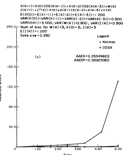
X(K+I)=X(K)COS(X(K-I))+X(K-2)COS(X(K-3))+W(K) Z(K)=(I+12(K))X(K)+X(K-l)X(K-2)tX(K-3)tV(K) E(X(O))=E(X(-I))=E(X(-2))_E(X(-3))=l.200 VAR(X(O))=VAR(X(-l))=VAR(X(-2))=VAR(X(-3))=0.500 VAR(V(K))=3.000.VAR(W(K))=2.900,

VAR(I(K))=O.bOO .Num.of disc.for W(K)=3,X(0)=3, I(K)=3 E(I(K))=l.200 Gate size = 0.250 Legend q ER.COV. (b) Bound=0 13414E-2

K. Demirba? X(K+I)=X(K)COS(X(K-I))+X(K-2)COS(X(K-3))+W(K) Z(K)=(I +I’(K))X(K)+X(K-I)XfK-2)+X(K-3)+V(K) 240 200 160 .O- o- .o - .o- .o- .O- VARtVtK))-3.0OO.VAR(W(K)b2.900,VAR(I(~j)=0~S00 Num.of disc.for W(K)=3.X(0)=3, I(K)=3 E(I(K))=l.200

Gote sire = 0.250 Legend

A Kalman A ODSA Cc) AAEK10.253496E2 AAEOP=O,93925OEO b 0 1.20 2.40 3.60 4.60 6.00 Time

FIG. 4(c). Absolute and time-averaged absolute errors for estimates of states.

VI. Conclusions

The proposed estimation approach can be used to estimate the state of dynamic

models with both an Nth order memory and nonlinear random interference,

whereas the classical estimation schemes, such as the Kalman filter, in general,

cannot. Dynamic models of the proposed approach can be any nonlinear functions.

However, the implementation of the proposed estimation approach requires an

exponentially increasing memory with time.

References

(1) R. E. Kalman, “A new approach to linear filtering and prediction problems”, Trans.

ASME, J. Basic Eng., Ser. D., Vol. 82, pp. 3545, 1960.

(2) R. E. Kalman and B. C. Bucy, “New results in linear filtering and prediction theory”,

Trans. ASME, J. Basic Eng., Ser. D, Vol. 83, pp. 955108, 1961.

828

Journal of the FrankIn Institute Pergaman Press plc

(3) A. P. Sage and J. L. Melsa, “Estimation Theory with Applications to Communications

and Control”, McGraw-Hill, New York, 1971.

(4) T. Kailath, “An innovation approach to least square estimation, Part 1 : Linear filtering

in adaptive white noise”, IEEE Trans. Aut. Contr., Vol. AC-13, No. 6, pp. 646655, 1968.

(5) T. Kailath, “A view of three decades in linear filtering theory”, IEEE Trans. Znj:

Theory, Vol. IT-20, No. 2, pp. 146181, 1974.

(6) J. Makhoul, “Linear prediction : A tutorial review”, Proc. IEEE, Vol. 63, pp. 561-

580, 1975.

(7) J. S. Medich, “A survey of data smoothing for linear and nonlinear dynamic systems”,

Automatica, Vol. 9, pp. 151-162, 1973.

(8) C. E. Hutchinson, “The Kalman Filter applied to aerospace and electronic systems”,

IEEE Trans. Aerospace Electron. Syst., Vol. AES-20, No. 4, pp. 500-504, 1984.

(9) N. E. Nahi, “Optimal recursive estimation with uncertain observation”, IEEE Trans.

Znf Theory, Vol. IT-15, No. 4, pp. 457462, 1969.

(10) R. A. Monzingo, “Discrete optimal linear smoothing for systems with uncertain

observation”, IEEE Trans. Inf Theory, Vol. IT-21, No. 3, pp. 271-275, 1975.

(11) K. Demirbag, “Information theoretic smoothing algorithms for dynamic systems with

or without interference”, Adv. Contr. Dyn. Syst., Volume XXI, pp. 1755295, Aca-

demic Press, New York, 1984.

(12) K. Demirbas and C. T. Leondes, “Optimum decoding based smoothing algorithm for

dynamic systems with interference”, Int. J. Syst. Sci., Vol. 17, No. 2, pp. 251-267,

1986.

(13) H. L. Van Trees, “Detection, Estimation and Modulation Theory”, Wiley, New York,

1968.

(14) G. D. Forney Jr, “Convolution codes II. Maximum likelihood decoding”, Inf. Contr.,

Vol. 25, pp. 222-266, 1974.

(15) A. J. Viterbi and J. K. Omura, “Principles of Digital Communication and Coding”,

McGraw-Hill, New York, 1979.

(16) R. G. Gallager, “A simple derivation of the coding theorem and some applications”,

IEEE Trans. Zn$ Theory, Vol. IT-l 1, pp. 3-18, 1965.

Vol. 326. No. 6, pp. 817-829, 1989