A NONLINEAR CONTROL SCHEME FOR DISCRETE TIME CHAOTIC SYSTEMS
Ömer Morgül
Bilkent University, Dept. of Electrical and Electronics Engineering, 06800, Bilkent, Ankara, Turkey
Abstract: In this paper we consider the stabilization problem of unstable periodic orbits of discrete time chaotic systems. We consider both one dimensional and higher dimensional cases. We propose a nonlinear feedback law and present some stability results. These results show that for period 1 all hyperbolic periodic orbits can be stabilized with the proposed method. By restricting the gain matrix to a special form we obtain some novel stability results. The stability proofs also give the possible feedback gains which achieve stabilization. We also present some simulation results.
Keywords: Chaotic Systems, Chaos Control, Delayed Feedback System, Pyragas Controller, Stability.
1. INTRODUCTION
The study of dynamical systems has always been an area which attracts scientist from different disciplines including engineers, mathematicians, physicists, etc. Because of the fact that many systems exhibit chaotic behaviours, the study of such systems has received considerable attention in recent years, see e.g. (Chen and Dong, 1999), (Fradkov and Evans, 2002), and the references therein. Since chaotic systems exhibit quite interesting behaviours, various aspects of such sys-tems have been investigated in the literature. Among these the feedback control of chaotic systems received great interests among scientists from various disci-plines after the seminal work of (Ott, Grebogy and Yorke, 1990). After the latter work, various other con-tributions have appeared in the area of chaos control. The literature is quite rich on this subject, see e.g. (Chen and Dong, 1999), (Fradkov and Evans, 2002), and the references therein.
Chaotic systems may exhibit quite large number of interesting behaviours. One of such interesting fea-tures which is a characteristic behaviour of chaotic
systems is that they usually possess attractors which are called "strange" due to various reasons. Such at-tractors usually contain infinitely many unstable peri-odic orbits, (Devaney, 1987). An interesting result first given in (Ott, Grebogy and Yorke, 1990) proved that some of these unstable orbits could be easily stabi-lized by applying small control inputs to such systems. Following the latter result various control schemes for the stabilization of unstable periodic orbits of chaotic systems have been proposed, see e.g. (Chen and Dong, 1999), (Fradkov and Evans, 2002), and the references therein. Among these works, the Delayed Feedback Control (DFC) scheme, first proposed by Pyragas in (Pyragas, 1992) has received considerable attention due to its various attractive features as well as its simplicity. The study of DFC revealed that this scheme has some inherent limitations, that is it can-not stabilize certain type of unstable periodic orbits, see e.g. (Morgül, 2003), (Ushio, 1996), (Nakajima, 1997), (Morgül, 2005a). We note that a recent result presented in (Fiedler et al., 2007), showed clearly that under certain cases, odd number limitation property does not hold for autonomous continuous time sys-tems. Although the subject is still open and deserves
further investigation, we note that the limitation of DFC stated above holds for discrete time case, see e.g. (Ushio, 1996), (Morgül, 2003), (Morgül, 2005a). To eliminate the limitations of DFC indicated above, different modifications and/or extensions have been proposed, see e.g. (Pyragas, 1995), (Pyragas, 2001), (Socolar et. al., 1994), (Bleich, and Socolar, 1996), (Vieira, and Lichtenberg, 1996), and the references therein. Among such modifications, the periodic feed-back scheme proposed in (Schuster and Stemmler, 1997) eliminates those limitations for period 1 case and it could be generalized to higher period cases in various ways. Two such generalizations are given in (Morgül, 2006), (Morgül, 2005b) and it has been shown in that any hyperbolic periodic orbit can be stabilized with these schemes. Another modification is the so-called extended DFC (EDFC), see (Soco-lar et. al., 1994). It has also been shown that EDFC also has inherent limitations similar to the DFC. In (Vieira, and Lichtenberg, 1996), a nonlinear version of EDFC has been proposed and it was shown that an optimal version of this scheme becomes quite simple. A generalization of this scheme for arbitrary periodic orbits for one dimensional systems has been given in (Morgül, 2009a). Preliminary results of the extension of these ideas to higher dimensional case for the latter approach has been presented in (Morgül, 2009b). In this paper we will elaborate on the nonlinear scheme proposed in (Morgül, 2009a) and (Morgül, 2009b) by considering the stabilization of arbitrary periodic orbits of multi dimensional discrete time chaotic systems. Instead of a simulation based search for the stabilizing gains used in (Morgül, 2009b), we will provide an approach which is more systematic. This paper is organized as follows. In section 2 we will outline the basic problem considered and introduce some notation used throughout the paper. In section 3 we will introduce the nonlinear controller for the one dimensional case and present some stability results. In section 4 we will present the generalization of this scheme to higher dimensional case and provide some stability results. Then we will present some simula-tion results and finally we will give some concluding remarks.
2. PROBLEM STATEMENT
Let us consider the following discrete-time system x(k + 1) = f (x(k)) , (1)
where k = 1,2 ... is the discrete time index, x ∈ Rn, f :
Rn→ Rnis an appropriate function, which is assumed to be differentiable wherever required. We assume that the system given by (1) possesses a period T orbit characterized by the set
ΣT = {x∗1, x∗2, . . . , x∗T} , (2)
where x∗
i ∈ Rn, i = 1, 2, . . . , T .
Let x(·) be a solution of (1). To characterize the con-vergence of x(·) to ΣT, we need a distance measure, which is defined as follows. For x∗
i, we will use circu-lar notation, i.e. x∗
i = x∗j for i = j (mod (T )). Let us define the following indices ( j = 1,...,T ):
dk( j) = s T−1
∑
i=0 kx(k + i) − x∗ i+ jk2 , (3)where k · k is the standard Euclidean norm on Rn. We then define the following distance measure
d(x(k), ΣT) = min{dk(1), . . . , dk(T )} . (4)
Clearly, if x(1) ∈ ΣT, then d(x(k),ΣT) = 0, ∀k. Con-versely if d(x(k),ΣT) = 0 for some k0, then it remains 0 and x(k) ∈ ΣT, for k ≥ k0. We will use d(x(k),ΣT) as a measure of convergence to the periodic solution given by ΣT.
Let x(·) be a solution of (1) starting with x(1) = x1. We say that ΣT is (locally) asymptotically stable if there exists anε> 0 such that for any x(1) ∈ Rnfor which
d(x(1), ΣT) <εholds, we have limk→∞d(x(k), ΣT) = 0. Moreover if this decay is exponential, i.e. the fol-lowing holds for some M ≥ 1 and 0 <ρ< 1, (k > 1)
d(x(k), ΣT) ≤ Mρkd(x(1), ΣT) , (5)
then we say that ΣT is (locally) exponentially stable. To stabilize the periodic orbits of (1), let us apply the following control law :
x(k + 1) = f (x(k)) + u(k) (6)
where u(·) ∈ Rnis the control input. In classical DFC, the following feedback law is used (k > T ):
u(k) = K(x(k) − x(k − T )) , (7)
where K ∈ Rn×nis a constant gain to be determined. It is known that the scheme given above has certain in-herent limitations, see e.g. (Ushio, 1996). For simplic-ity, let us assume one dimensional case, i.e. n = 1. For ΣT, let us set ai= f′(x∗i). It can be shown that ΣT can-not be stabilized with this scheme if a = ∏T
i=1ai> 1, see e.g. (Morgül, 2003), (Ushio, 1996), and a similar condition can be generalized to the case n > 1, (Naka-jima, 1997), (Morgül, 2005a). A set of necessary and sufficient conditions to guarantee exponential stabi-lization can be found in (Morgül, 2003) for n = 1 and in (Morgül, 2005a) for n > 1. By using these results one can find a suitable gain K when the stabilization is possible.
3. A NONLINEAR GENERALIZATION OF DFC To simplify our analysis we first consider one dimen-sional case, i.e. n = 1 throughout this section.
Con-sider the system given by (1). First conCon-sider a period 1 orbit Σ1of (1) (i.e. fixed point of f : R → R) given by Σ1= {x∗1}. Instead of control law given by (7), let us consider the following control law :
u(k) = K
K+ 1(x(k) − f (x(k)) , (8)
where K ∈ R is a constant gain to be determined. Obviously we require K 6= −1. By using (8) in (6), we obtain :
x(k + 1) = 1
K+ 1f(x(k)) + K
K+ 1x(k) . (9)
Obviously on Σ1, we have u(k) = 0, see (8). Further-more if x(k) → Σ1(i.e. when Σ1is asymptotically sta-ble) we have u(k) → 0 as well. Therefore, the scheme proposed in (8) enjoys the similar properties of DFC. To analyze the stability of Σ1, let us define a = a1=
f′(x∗1). By using linearization, (9) and the classical Lyapunov stability analysis, we can easily show that Σ1is locally exponentially stable for (9) if and only if
|K+ a
K+ 1 |< 1 . (10)
It can easily be shown that if a 6= 1, then any Σ1can be stabilized by choosing K appropriately to satisfy (10), see e.g. (Morgül, 2009a) and (Morgül, 2009b). This shows that any hyperbolic periodic orbit can be stabilized with the proposed scheme for T = 1 case. The scheme proposed above for T = 1 case could be generalized to period m case as follows :
u(k) = K
K+ 1(x(k − m + 1) − f (x(k)) , (11) where K ∈ R is a constant gain to be determined. If we use (11) in (6), we obtain :
x(k + 1) = 1
K+ 1( f (x(k)) + Kx(k − m + 1)).(12)
Now let us assume that period m orbit Σm of (1) be given as in (2). Let us define ai = f′(x∗i), i = 1,2,...,n, and a = ∏i=n
i=1ai. Let us define the following characteristic polynomial pm(·) associated with the system given by (6) and (11) as follows :
pm(λ) = (λ− K K+ 1) m− a (K + 1)mλ m−1 . (13)
A polynomial is called as Schur stable if all of its roots are strictly inside the unit disc of the complex plane, i.e. the roots have magnitude strictly less than 1. As is well known, by using Lyapunov stability theory local stability can be analyzed by using the Schur stability of an appropriately defined characteristic polynomial, see e.g. (Khalil, 2002). The next theorem is a result of such an analysis.
Theorem 1 : Let Σm given by (2) be a period T = m orbit of (1) and set ai = f′(xi), i = 1, 2, . . . , m, a = ∏mi−1ai. Consider the control scheme given by (6) and (11). Then :
i : Σm is locally exponentially stable if and only if
pm(λ) given by (13) is Schur stable. This condition is only sufficient for asymptotic stability.
ii : If pm(λ) has at least one unstable root, i.e. outside the unit disc, then Σmis unstable as well.
iii : If pm(λ) is marginally stable, i.e. has at least one root on the unit disc while the rest of the roots are inside the unit disc, then the proposed method to test the stability of Σmis inconclusive.
Proof : The proof of this Theorem easily follows from standard Lyapunov stability arguments, see e.g. (Khalil, 2002), and (Morgül, 2003), (Morgül, 2005a), (Morgül, 2009a) and (Morgül, 2009b) for similar ar-guments. 2
Associated with (13), let us define the following con-stants Kcr= −0.5 + 0.5(| a |)1/m , (14) amcr= ( m m− 2) m . (15)
Given a and m, by studying the relation between the roots of pm(·) given by (13) and the gain K, we obtain the following results.
Theorem 2 : Let a and m be given and consider the polynomial pm(·) given by (13).
i : If K is a stabilizing gain, then K + 1 > 0.
ii : If a > 1, then stabilization is not possible, (i.e. pm(·) is not Schur stable for any K).
iii : If | a |< 1, pm(·) is Schur stable for any K ≥ 0.
iv : For K ≤ Kcr, stabilization is not possible.
v : If −amcr< a < 1, then there exits a Km> Kcrsuch that pm(·) is Schur stable for Kcr< K < Km.
Proof : For stability of pm(·), a necessary condition is to have | pm(0) |< 1, see e.g. (Elaydi, 1996). This im-plies K + 1 > 0 should hold, which proves i. Another necessary condition for stability is that pm(1) > 0 should hold, see e.g. (Elaydi, 1996). Together with K+ 1 > 0, this implies that 1 − a > 0 should hold, which proves ii . When | a |< 1, Σmis already stable for K = 0. This could also be seen from (13), since m− 1 roots of pm(·) are at 0 and the last one is at a when
K= 0. By analyzing the roots of pm(·) (e.g. by using Rouchè’s theorem), it can be shown that all of the roots of (13) are inside the unit disc for K ≥ 0, which proves iii. Another necessary condition for Schur stability is to have (−1)mp
m(−1) > 0, see e.g. (Elaydi, 1996). By using the latter, together with K + 1 > 0, we obtain K> Kcr, which proves iv. To prove v, one can show that when K = Kcr, m − 1 roots of pm(·) are strictly
inside the unit disc and the last one is at −1. Then by using some continuity arguments. we can show that for K = Kcr+εwhereε> 0 is sufficiently small, pm(·) is Schur stable, which proves v. 2
4. EXTENSION TO HIGHER DIMENSIONAL CASE
The stabilization scheme given in the previous section can be generalized to higher dimensional case by changing K from being a scalar to a gain matrix. For motivation, as in the previous section let us consider a period 1 orbit Σ1of (1) given by Σ1= {x∗1}, where
x∗1∈ Rnis a fixed point of f : Rn→ Rn. One possible generalization of the control law given by (11) is the following :
u(k) = (K + I)−1K(x(k) − f (x(k)) , (16)
where K ∈ Rn×n is a constant gain matrix to be de-termined, and I is n × n identity matrix. Obviously K+ I should be nonsingular, i.e. K should not have an eigenvalue −1. By using (16) in (6) we obtain :
x(k + 1) = (K + I)−1( f (x(k)) + Kx(k)) . (17)
For stability analysis, let us define : J=∂f
∂x |x=x∗1 . (18)
Let us define e = x − x∗
1. By using linearization, from (17) we obtain :
e(k + 1) = Ae(k) , (19)
where A = (I + K)−1(J + K). Clearly the error dynam-ics given by (19) is locally exponentially stable if A given above have all of its eigenvalues in the unit disc. The characteristic polynomial associated with A can be given as :
p1(λ) = det(λI− A)
= det[(λI− (I + K)−1K) −(I + K)−1J]
(20)
which is similar to (13) for n = 1. However, estab-lishing a similar relation for the case m > 1 is not straightforward. First note that if J does not have an eigenvalue 1, then by choosing K appropriately, p1(λ) can be made stable. Indeed, if ∆ is any Schur stable matrix, then K = (I − ∆)−1(∆ − J) is such a stabilizing gain matrix, (Morgul, 2009b). Hence the limitations of DFC are greatly eliminated with the proposed scheme; in fact any hyperbolic fixed point can be stabilized with the proposed approach.
Moreover, if K is constrained to the form K =εI, then (20) reduces to :
p1(λ) = det[(λ− ε
ε+ 1)I −
1
ε+ 1J] , (21)
for which the similarity with (13) is more apparent. In this case, the roots of p1(λ) given by (21) are the same as the eigenvalues of Jε = εI+Jε+1. Let the eigenvalues of J be given as λ1, . . . ,λn. Then the eigenvalues of
Jε are ε+λε+1i, i = 1,2,...,n. Clearly for stabilization we require : | ε+λi
ε+1 |< 1, i = 1, 2, . . . , n. If all λi are real, andλi< 1, then by choosingε> 0 sufficiently high, we can always find a stabilizing gain of the form K=εI. On the other hand, if some eigenvalues of J are complex, then a similar analysis would be more complicated and due to space limitations this part of the analysis is omitted here.
The control law given by (16) could be generalized to higher order periods T = m > 1 as follows :
u(k) = (K + I)−1K(x(k − m + 1) − f (x(k)) .(22)
Let Σm= {x∗1, . . . , x∗m} be such a period m orbit of (1). Let us define the following Jacobians :
Ji=
∂f
∂x |x=x∗i , i = 1, .., m , J = J1.J2..Jm . (23)
Stability of Σm for the system given by (6) and (22) becomes rather complex. We follow the methodology given in (Morgul, 2003), (Morgul, 2005a). Let us define the variables xias follows :
xi(k) = x(k − m + i) , i = 1, . . . , m . (24)
By using (24), let us define z = (xT
1..xTm)T ∈ Rnm. Let us define the following variables (for i = 1,...,m) :
Y0= xm , (25)
Yi= (I + K)−1f(Yi−1) + (I + K)−1Kxi . (26)
Now let us define a map F : Rnm→ Rnmas follows :
F(z) = (xT
2xT3...xTmY1T)T . (27) It can easily be shown that Fm(z) = (YT
1...YmT)T. Also it can be shown that Σm now corresponds to a fixed point of Fm. More precisely, corresponding to Σ
m, let us define a vector z∗= (x∗T
1 ..x∗Tm )T. It is easy to show that z∗ is a fixed point of Fm. It then can easily be shown that the stability of Σmfor (6) and (30) can be analyzed by considering the stability of the fixed point z∗ of Fm. For the latter, let us define the following Jacobian matrix :
JF=
∂Fm
∂z |z=z∗ , (28)
and define the characteristic polynomial pm(·) as fol-lows :
pm(λ) = det(λI− JF) . (29)
Theorem 3 : Let Σmbe a period m orbit of (1). Con-sider the system given by (6) and (22). Then, Σm is
locally exponentially stable if and only if the charac-teristic polynomial given by (29) is Schur stable. Proof : The proof of this Theorem easily follows from standard Lyapunov stability arguments, see e.g. (Khalil, 2002), and (Morgül, 2003), (Morgül, 2005a), (Morgül, 2009a) for similar arguments. 2
Obtaining a better expression for pm(·) given by (29) for an arbitrary gain matrix K is not straightforward. For the special case of K =εI, after some straightfor-ward calculations we obtain the following :
pm(λ) = det[(λ−
ε
ε+ 1)
mI− λm−1
(ε+ 1)mJ] , (30)
where J is given by (23). Clearly, if n = 1, then (30) reduces to (13).
For further development, let us assume that J has only real eigenvalues. Letλ1, . . . ,λn be these eigenvalues. Also let us define the following polynomials (for i = 1,...,n) : pmi(λ) = (λ− ε ε+ 1) m− λm−1λi (ε+ 1)m . (31) It can easily be shown that the following holds :
pm(λ) = n
∏
i=1
pmi . (32)
If we can find anεsuch that all pmi(·) are Schur stable, then K =εIwill be a stabilizing gain. Based on this observation, we can state the following result. Theorem 4 : Let Σm be a period m solution of (1), and consider the system given by (6), (22). Consider the Jacobian J associated with Σm as defined in (23) and assume that J has only real eigenvalues given as λ1, . . . ,λn. If −amcr <λi< 1, i = 1, . . . , n, where
amcr is given by (15), then there exist two constants
εmax >εmin such that K =εIis a stabilizing gain for Σm; hereεmin<ε<εmax.
Proof : The proof follows from the results given in section 3 and the developments given above. See also Theorem 2. 2
5. SIMULATION RESULTS
As a simulation example, we consider the coupled map lattices, which exhibit various interesting dynam-ical behaviours. We will use the following coupled lattice system :
x(k + 1) = f (x(k)) +α( f (y(k)) − f (x(k))), (33) y(k + 1) = f (y(k)) +α( f (x(k)) − f (y(k))), (34)
where f (·) is the tent map given as f (z) = mz for z≤ 0.5, and f (z) = m − mz for 0.5 < z ≤ 1. For
m= 1.9 andα = 0.1, this map has period 3 solution characterized by the set Σ3= {w∗1, w∗2, w∗3} where w∗i = ( x∗i y∗i )T, i = 1,2,3 and x∗1= 0.8966, y∗1= 0.642793,
x∗2 = 0.24467, y∗
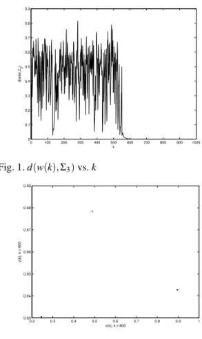
2= 0.6304685, x∗3 = 0.48859, y∗3= 0.678386. The associated Jacobian matrix J given by (23) could easily be found. The eigenvalues of J can be found asλ1= −4.3898,λ2= −5.4872. Note that a3cr can be found from (15) as 27, hence the conditions in the Theorem 4 are satisfied. By using (14), the critical gains K1crand K2crcorresponding toλ1andλ2could be found as K1cr = 0.3187 and K2cr = 0.3819. By using the polynomials defined in (31) on can show that stabilization is possible for gains of the form K =εI where 0.3819 <ε< 90. A typical simulation results were given in Figures 1-4. In these simulations, we chose ε= 0.4, x(0) = 0.8, y(0) = 0.6. In Figure 1, we show d(w(k),Σ3) versus k, and as can be seen the decay is exponential. Figure 2 shows x(k) versus y(k) plot for k ≥ 800. As can be seen, solutions converge to Σ3. Finally Figure 3 and 4 show u1(k) and u2(k) vs. k.
0 100 200 300 400 500 600 700 800 900 1000 0 0.1 0.2 0.3 0.4 0.5 0.6 0.7 0.8 0.9 k d(w(k), Σ3 ) Fig. 1. d(w(k),Σ3) vs. k 0.2 0.3 0.4 0.5 0.6 0.7 0.8 0.9 1 0.63 0.64 0.65 0.66 0.67 0.68 0.69 x(k), k ≥ 800 y(k), k ≥ 800
Fig. 2. x(k) vs. y(k) for k ≥ 800
6. CONCLUSIONS
In this paper, we considered a generalization of the DFC scheme proposed in (Morgul, 2009a) to mul-tidimensional case. Such an attempt was first made in (Morgul, 2009b), but the results presented in the latter were rather preliminary in nature. In the present paper, we considered first one dimensional case for the proposed method and presented some conditions
0 100 200 300 400 500 600 700 800 900 1000 −0.04 −0.03 −0.02 −0.01 0 0.01 0.02 0.03 k u1 (k) Fig. 3. u1(k) vs. k 0 100 200 300 400 500 600 700 800 900 1000 −0.06 −0.04 −0.02 0 0.02 0.04 0.06 k u2 (k) Fig. 4. u2(k) vs. k
which guarantee the existence of a stabilizing gain. Based on these results, obtaining bounds for the stabi-lizing gains are rather straightforward. Then by using these results in multidimensional case we obtained some conditions which guarantee the existence of a stabilizing gain in the form K =εI. We also presented some simulation results.
7. REFERENCES
Bleich, M.E. , and Socolar, J.E.S. (1996), “Stability of periodic orbits controlled bt time delay feedback," Phys. Lett. A,210, pp 87-94.
Chen, G., and X. Dong, (1999) From Chaos to Order : Methodologies, Perspectives and Applications, World Scientific, Singapore.
Devaney, R. L. (1987), Chaotic Dynamical Systems, Addison-Wesley, Redwood City.
Elaydi, S.N. (1996), An Introduction to Difference Equations, Springer-Verlag, New York.
Fiedler, B., Flunkert, V., Georgi, M., Hövel, P. and Schöll, E. (2007) “Refuting the odd-number limitation of time-delayed feedback control," Phys. Rev. Lett, 98, PRL No : 114110.
Fradkov, A. L., and R. J. Evans (2002) “Control of Chaos : Survey 1997-2000," Proceedings of 15th IFAC World Congress, 21-26 July 2002, Barcelona, Spain, pp. 143-154.
Khalil, H. K. (2002) Nonlinear Systems, 3rd ed. Prentice-Hall, Upper Saddle River.
Morgül, Ö. (2003) “On the stability of delayed feed-back controllers," Phys. Lett. A314, 278-285.
Morgül, Ö. (2005a) “On the stability of delayed feed-back controllers for discrete time systems," Phys. Lett. A335, 31-42.
Morgül, Ö. (2005b) “On the stabilization of periodic orbits for discrete time chaotic systems," Phys. Lett. A335, 127-138.
Morgül, Ö. (2006) “Stabilization of unstable periodic orbits for discrete time chaotic systems by using peri-odic feedback," Int. J. Bifurcation Chaos 16, 311-323. Morgül, Ö. (2009a) “A New Generalization of De-layed Feedback Control," Int. J. Bifurcation Chaos, 16, 365-377.
Morgül, Ö. (2009b) “ A New Delayed Feedback Con-trol Scheme for Discrete Time Chaotic Systems," Pro-ceedings of 2nd IFAC Conf. on Anal. and Cont. of Chaotic Systems, 22-24 June 2009, London, England. Nakajima, H. (1997) “On analytical properties of de-layed feedback control of chaos," Phys. Lett. A232, 207-210.
Ott, E., C. Grebogi, and J. A. Yorke (1990) “Control-ling Chaos," Phys. Rev. Lett., 64, pp. 1196-1199. Pyragas, K. (1992) “Continuous control of chaos by self-controlling feedback," Phys. Lett. A., 170, pp. 421-428.
Pyragas, K., (1995), “Control of chaos via extended delay feedback," Phys. Lett. A, 206, pp. 323-330. Pyragas, K. (2001) “Control of chaos via an unstable delayed feedback controller," Phys. Rev. Lett., 86 pp. 2265-2268.
Socolar, J. E., Sukow, D. W., and Gauthier, D. J., (1994), “Stabilizing unstable periodic orbits in fast dynamical systems," Phys. Rev. E., vol. 50, pp. 3245-3248.
Ushio, T. (1996) “Limitation of delayed feedback con-trol in nonlinear discrete time systems," IEEE Trans. on Circ. Syst.- I 43, 815-816.
Vieira, d.S.M, & Lichtenberg, A.J. (1996) “Control-ling chaos using nonlinear feedback with delay," Phys. Rev. E54, 1200-1207.