Nonlinear hierarchical control of a quad tilt-wing UAV: An adaptive control approach

DOI: 10.1002/acs.2759

R E S E A R C H A R T I C L E

Nonlinear hierarchical control of a quad tilt-wing UAV: An

adaptive control approach

Yildiray Yildiz

Mustafa Unel

Ahmet Eren Demirel

1_{Department of Mechanical Engineering, Bilkent}

University, Cankaya, Ankara 06800, Turkey

2_{Faculty of Engineering and Natural Sciences,}

Sabanci University, Tuzla, Istanbul 34956, Turkey

Correspondence

Mustafa Unel, Faculty of Engineering and Natural Sciences, Sabanci University, Tuzla, Istanbul 34956, Turkey.

Email: munel@sabanciuniv.edu

Summary

In this paper, a nonlinear hierarchical adaptive control framework is proposed for the control of a quad tilt-wing unmanned aerial vehicle (UAV). An outer loop model reference adaptive controller with robustifying terms creates required forces to be able to move the UAV on a reference trajectory, and an inner loop nonlinear adaptive controller realizes the required attitude angles to achieve these forces. A rigorous sta-bility analysis is provided showing the boundedness of all the signals in this cascaded controller structure. The development and the stability analysis of the controller do not use any linearizations and use the full nonlinear UAV dynamics. The controller is implemented on a high-fidelity nonlinear tilt-wing quadrotor model in the pres-ence of uncertainties, wind disturbances, and measurement noise as well as actuator and structural failures. In this work, in addition to earlier modeling studies, the effect of wing-angle variations, actuator failures, and structural failures and their effect on the center of gravity of the UAV are rigorously and systematically investigated and reflected in the model. Simulation results showing the performance of the pro-posed controller and a comparison with the fixed controller used in earlier studies are presented in the paper.

K E Y W O R D S

adaptive control, hierarchical control, MRAC, tilt-wing UAV, VTOL

1 I N T R O D U C T I O N

Significant progress has been made in the design, modeling, and control of unmanned aerial vehicles (UAVs) in the last decade, and much recent work has been devoted to the inves-tigation of hybrid-wing UAVs. Hybrid-wing UAVs are plat-forms where the advantages of rotary-wing and fixed-wing UAVs are combined: They can achieve vertical takeoff and

Nomenclature: m, mass, kg; Ib, inertia matrix in the body frame, kg·m2; Vw, linear velocity in the world frame, m/s; Ωb, angular velocity in the body frame, rad/s;Ωw, angular velocity in the world frame, rad/s; Ft, net force, N; Mt, net moment, N·m; X, Y, Z, coordinates of the center of mass in the world frame, m; p, q, r, angular velocities in the body frame, rad/s; Φ,Θ,Ψ, roll, pitch and yaw angles in the world frame, rad; 𝜔i, rotational speed of the ithrotor, rad/s; M, inertia matrix; 𝜁, vector defined as[Ẋ ,̇Y,Ż , p, q, r]T _{; 𝜉, vector defined as [X, Y, Z,Φ,Θ,Ψ]}T_{; C(𝜁), Coriolis-centripetal matrix; G, gravity} vector, m·s−2_{; I}

xx, Iyy, Izz, moments of inertia around the body axes, kg·m2; O(𝜁,𝜔i), gyroscopic term; E(𝜉, 𝜔2i), actuator vector; 𝜃f, front wing angle, rad;

k, motor thrust constant, N·s2_·rad−2_{; l}

s, rotor distance to center of mass along y axis, m; ll, rotor distance to center of mass along x axis, m; 𝜆, torque/force

ratio; W(𝜉), wing force vector, N; Rbw, rotation matrix representing the orientation of the body frame w.r.t. world frame; FD,FL, drag and lift forces, N;

vx, vy, vz, linear velocities in the body frame, m/s; ̇X, ̇Y, ̇

Z, linear velocities in the world frame, m/s; v𝛼, variable defined as √

v2

x+ v2z;𝜃i, wing angle of attack w.r.t. body x axis, rad; 𝛼i, effective angle of attack of the wing w.r.t. air flow, rad; 𝜌, air density, kg·m−3; A, wing planform area, m2; R(𝜃i−𝛼i), rotation matrix around body y axis; 𝛼w, vector defined as [Φ,Θ,Ψ]T; E(𝛼w), velocity transformation matrix between from the world frame to the body frame.

landing (VTOL) without the assistance of any special infras-tructure, and they can fly for extended periods with high speed. A subclass under the hybrid-wing UAVs is tilt-rotor UAVs, which constitute the characteristic of efficient energy use.1,2_{In this subclass, one can find dual tilt-rotor}3_{and dual}

tilt-wing UAVs.4_{Quad-tilt wing UAVs}5,6_{form another}

cate-gory, which do not show the disadvantage of cyclic control requirement that can be seen in its dual tilt-rotor counterparts.

The couplings between the translational and rotary motions, highly nonlinear multi-input multioutput system dynamics, uncertainty sources such as unpredictable damages, and actu-ator malfunctions7 _{are challenges that make the control of}

tilt-wing UAVs a difficult task, which requires advanced con-trollers if high performance throughout a large flight envelope is demanded. There exists a rich literature on the closed-loop control of rotary UAVs offering a variety of controllers to handle these challenges. Some examples of controllers pro-posed in the literature are proportional-integral-derivative (PID)–type controllers,8-11 _{PD2 controllers where a}

propor-tional and 2 derivative actions are used,12 _{linear quadratic}

regulator controllers,9,13-15_{sliding mode observers with}

feed-back linearization,16

H∞controllers,17

feedback linearization approaches,18 _{nonlinear model predictive control,}19_dynamic

inversion with 𝜇 synthesis,20 _{nested nonlinear controllers,}21

backstepping approaches,22-24_{and some other nonlinear}

con-trol techniques.25_{There are other control methods proposed in}

the literature that use a hierarchical structure26-30_{with various}

types of controllers for rotational and translational dynamics. An excellent comprehensive literature survey about the guid-ance, navigation, and control of rotary UAVs can be found in 1 study.31

All the above-mentioned control approaches proved suc-cessful in simulation and experimental environments for spe-cific operating conditions. The proposed controller in this paper is built upon these earlier works by eliminating the precise plant model requirement for the optimization-based and classical approaches and by eliminating the conservatism introduced by the robust control approaches. This is achieved by using a hierarchical nonlinear adaptive controller where adaptive controllers are used both for the translational and rotational motion control and thus providing adaptation in all 6 degrees of freedom, together with a rigorous stability analysis for the overall cascaded closed-loop system. There exist other adaptive control approaches in the literature for the control of rotary UAVs such as the ones proposed in previ-ous studies32-35 _{and a very recent one in the work of Dydek}

et al.7_{However, the hierarchical adaptive control framework}

proposed in this paper is different from them: Unlike in the work of Johnson and Kannan,32 _{the proposed control}

framework does not use any neural networks and therefore

computationally less expensive; unlike this study,33_{no small}

angle or slowly varying parameter assumptions are made; unlike another study,34_{no fuzzy approximators are used and}

again, computationally cheaper; unlike another study,35

uncer-tainties in both the translational and rotational motion are addressed, and finally, unlike this study,7 _{no linearization}

is conducted on plant dynamics. In addition, none of these mentioned adaptive control approaches are implemented on a tilt-wing UAV.

It is known that the problem of nonlinear controllers, in gen-eral, is computational complexity.36_{The focus of this paper}

is the design of a high-performance, practical controller that is easy to implement with low computational cost but at the same time theoretically sound that does not need any lin-earization approximation of the plant dynamics and that has a rigorous overall stability proof. In addition, the proposed controller is able to compensate the uncertainties in plant dynamics, due to online wing-angle variations, damages, and unexpected component failures. All these features are realized by using 2 adaptive controllers in cascade: A model refer-ence adaptive control (MRAC) design for the translational dynamics and a nonlinear adaptive controller for the rotational dynamics. Although these approaches are well known, their cascaded implementation in a hierarchical framework for the hybrid-wing UAVs has not been shown to result in a stable closed-loop system before, to the best of authors’ knowledge. The proof of stability of this overall closed-loop system is achieved by the help of lumping the inner loop errors as a disturbance term and using robustifying terms in the adaptive controller design. Therefore, the implementation of 2 com-putationally cheap adaptive controllers in a cascaded form together with a stability proof provides the well-needed con-trol framework, which is practical, adaptive, and theoretically sound at the same time.

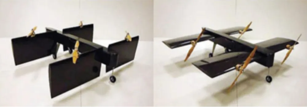
The proposed control framework is implemented for the control of a novel quad tilt-wing UAV (SUAVI: Sabanci Uni-versity Unmanned Aerial Vehicle), shown in Figure 1. The characteristics that make SUAVI a novel quad tilt-wing UAV and its advantages over existing designs can be found in 1 study.37 _{Sabanci University Unmanned Aerial Vehicle was}

previously designed, manufactured, and flight tested by Unel et al, and earlier research results have been published about

FIGURE 1 Quad tilt-wing unmanned aerial vehicle (Sabanci University Unmanned Aerial Vehicle) with 2 different wing-angle configurations. [Colour figure can be viewed at wileyonlinelibrary.com]

the aerodynamic and mechanical design, prototyping, con-trol system design, and flight tests.37-40 _{However, in those}

studies, the effects of wing-angle variations, component fail-ures, and unexpected damages on system uncertainty were not investigated and the controller was not tested against these adverse conditions. The designed controller was a fixed controller without any adaptation capability and thus had lim-ited capabilities to compensate for uncertainties. In addition, although showed promising results in flight tests, the overall closed-loop control system did not have a rigorous stabil-ity proof and relied on the time-scale separation between the inner and outer loop controllers. In this paper, SUAVI is tested, via a high-fidelity simulation model, which was used during the development of the actual prototype, for the above-mentioned adverse conditions using a theoretically sound controller. Especially, the effect of wing-angle vari-ations on system dynamics is rigorously analyzed and the uncertainty it produces when combined with possible asym-metry between the wings and probable failures is quantified. A systematic study of wing-angle variations for tilt-wing UAVs and its effect on the adaptive closed loop control sys-tem was not rigorously investigated before. This is especially important during the transition phase between the vertical and the horizontal motions where the wings move from a vertical position (quadrotor behavior, Figure 1, left picture) to almost horizontal position (fixed-wing behavior, Figure 1, right pic-ture). This investigation also proposes a method of transition from the quadrotor mode to fixed-wing mode. In addition, energy conservation, compared to conventional quadrotors, with the help of lift creation with wings during horizontal flight is quantified.

To summarize, the contributions of this study are the fol-lowing. On the theory side, a novel nonlinear hierarchical adaptive controller is proposed where (1) each controller is computationally cheap, (2) both the overall hierarchical framework and individual controllers are easy to implement, (3) no linearization is needed in plant dynamics, and (4) over-all closed-loop stability proof is provided. To the best of authors’ knowledge, no such combination of adaptive con-trollers for a hierarchical control framework is used in earlier studies, especially with a rigorous stability proof. On the practical side, the proposed controller is implemented on a high-fidelity model of a novel quad tilt-wing UAV developed by the authors, where (1) uncertainties emanating from a com-bination of wing asymmetry, component failure, and unex-pected damages are quantified, (2) the effect of wing-angle variation during the transition phase on plant dynamics is quantified in a systematic manner, and (3) an approach is proposed for transition between the quadrotor phase (verti-cal wing) and the fixed-wing phase (almost horizontal wing). No earlier study exists about the adaptive control of quad tilt-wing UAVs that considers all these phenomena at the same time.

Preliminary simulation results of this study are presented in 1 study.41_{Different from the work of Yildiz et al,}41_{in this}

study, a rigorous stability analysis, implementation results with disturbances and noise, and a rigorous quantification of uncertainties due to wing movements and failures are presented.

The organization of the paper is as follows: System model is presented in Section 2. Controller design and stability investigation are presented in Section 3. Implementation scenario together with uncertainty quantification and trajec-tory generation is presented in Section 4. Simulation results are presented in Section 5, and a summary is given in Section 6.

2 S Y S T E M M O D E L

Equations of motion for the quad tilt-wing UAV are briefly presented in this section. A more detailed analysis can be found in 1 study.37_{Overall dynamic equations of the system}

are given as [ mI3×3 03×3 03×3 Ib ] [ ̇Vw ̇Ωb ] + [ 0 Ωb× (IbΩb) ] = [ Ft Mt ] , (1) where m and Ib represent the mass and the diagonal inertia matrix in the body frame and Vwand Ωb represent the linear and the angular velocities of the vehicle in the world and body frames, respectively. The net force and the moment applied on the vehicle are represented by Ftand Mt, respectively (see Figure 2). It should be noted that for tilt-wing quadrotors, these forces and moments are functions of the rotor trusts and wing angles.

Using vector-matrix notation, Equation 1 can be rewritten as follows: M ̇𝜁 + C(𝜁)𝜁 = G + O(𝜁, 𝜔i) + E(𝜉, 𝜔2_i) + W(𝜉), (2) where, 𝜁 = [ ̇X, ̇Y, Z, p, q, r]T_, (3) and 𝜉 = [X, Y, Z, Φ, Θ, Ψ]T_, (4) where X, Y, and Z are the coordinates of the center of mass with respect to the world frame, p, q, and r are the angular velocities in the body frame, Φ, Θ, and Ψ are the roll, pitch, and yaw angles of the vehicle expressed in the world frame, and𝜔i, i = 1, 2, 3, 4 represents the rotor rota-tional speeds. M, the inertia matrix, C, Coriolis-centripetal matrix, and G, the gravity term, are given as follows: M = [ mI3×3 03×3 03×3 diag (Ixx, Iyy, Izz) ] , (5)

FIGURE 2 Forces and moments on the quad tilt-wing unmanned aerial vehicle C(𝜁) = ⎡ ⎢ ⎢ ⎢ ⎢ ⎢ ⎣ 0 0 0 0 0 0 0 0 0 0 0 0 0 0 0 0 0 0 0 0 0 0 Izzr −Iyyq 0 0 0 −Izzr 0 Ixxp 0 0 0 Iyyq −Ixxp 0 ⎤ ⎥ ⎥ ⎥ ⎥ ⎥ ⎦ , (6) G = [0, 0, mg, 0, 0, 0]T, (7) where, Ixx, Iyy, and Izz are the moments of inertia around the body axes. The gyroscopic term, O(𝜁, 𝜔), is given as

O(𝜁, 𝜔i) = Jprop ⎛ ⎜ ⎜ ⎜ ⎝ 03×1 4 ∑ i=1 [𝜂iΩb× [ _c 𝜃i 0 −s_𝜃i ] 𝜔i ⎞ ⎟ ⎟ ⎟ ⎠ , (8)

where,𝜂(1,2,3,4)= 1, −1, −1, 1 and c_𝜃iand s_𝜃irepresent cosine and sine of the wing angles, respectively. When 2 simplifying assumptions are used, namely, neglecting the aerodynamic downwash effect of the front wings on the rear wings and using same angles for the front and rear wings, system actua-tor vecactua-tor, E(𝜉, 𝜔2_{), can be given as}

E(𝜉, 𝜔2_i) = ⎡ ⎢ ⎢ ⎢ ⎢ ⎢ ⎢ ⎣ (cΨcΘc𝜃f − (cΦsΘcΨ+ sΦsΨ)s𝜃f)u1 (sΨcΘc𝜃f − (cΦsΘsΨ− sΦcΨ)s𝜃f)u1 (−sΘc𝜃f − cΦcΘs𝜃f)u1 s_𝜃fu2− c𝜃fu4 s𝜃fu3 c_𝜃fu2+ s_𝜃fu4 ⎤ ⎥ ⎥ ⎥ ⎥ ⎥ ⎥ ⎦ , (9)

where𝜃frepresents front wing angle against the UAV body x-axis. Inputs u1, u2, u3, and u4in Equation 9 are given as

u1= k(𝜔2₁+𝜔2₂+𝜔2₃+𝜔2₄), (10)

u2 = kls(𝜔2₁−𝜔₂2+𝜔2₃−𝜔2₄), (11)

u3= kll(𝜔2₁+𝜔2₂−𝜔2₃−𝜔2₄), (12)

u4= k𝜆(𝜔2₁−𝜔2₂−𝜔2₃+𝜔2₄), (13)

where k, ls, ll, and𝜆 are the motor thrust constant, rotor dis-tance to center of mass along y-axis, rotor disdis-tance to center of mass along x-axis, and torque/force ratio, respectively.

The wing forces W(𝜉), lift and drag, and the moments they create on the UAV are given as

W(𝜁) = ⎡ ⎢ ⎢ ⎢ ⎢ ⎢ ⎢ ⎣ Rbw ⎡ ⎢ ⎢ ⎣ F_D1 + F2_D+ F3_D+ F_D4 0 F1_L+ F_L2+ F3_L+ F4_L ⎤ ⎥ ⎥ ⎦ 0 ll ( F1 L+ F 2 L− F 3 L− F 4 L ) 0 ⎤ ⎥ ⎥ ⎥ ⎥ ⎥ ⎥ ⎦ , (14)

where Rbwis the rotation matrix representing the orientation of the body frame with respect to world frame. The drag and lift forces, Fi D = F i D(𝜃f, vx, vz) and F i L = F i L(𝜃f, vx, vz), are given as ⎡ ⎢ ⎢ ⎣ F_Di 0 F_Li ⎤ ⎥ ⎥ ⎦ = R(𝜃i−𝛼i) ⎡ ⎢ ⎢ ⎣ −1 2cD(𝛼i)𝜌Av 2 𝛼 0 −1 2cL(𝛼i)𝜌Av 2 𝛼 ⎤ ⎥ ⎥ ⎦, (15) where v𝛼 = √

v2x+ v2z and𝛼i = 𝜃i− (−atan2(vz, vx)). Here,

𝜌 is the air density, A is the wing planform area and 𝛼iis the effective angle of attack of the wing with respect to the air flow, and𝜃i is the wing angle of attack with respect to the body x-axis. R(𝜃i−𝛼i) is the rotation matrix around y-axis that decomposes the forces on the wings on the body axis.

The relationship between the linear velocities in body frame

vx, vy, vz and linear velocities in the world frame ̇X, ̇Y, Z is given as [_v x vy vz ] = Rwb(Φ, Θ, Ψ) [ ̇X ̇Y Z ] . (16)

Using Equation 1, the following rotational dynamics, that is, in a form suitable for attitude controller design, is obtained:

where𝛼w = [Φ, Θ, Ψ]T, Ωw = [ ̇Φ, ̇Θ, ̇Ψ] and E(𝛼w) is the velocity transformation matrix, which is given as

E(𝛼w) = [ 1 0 −sΘ 0 cΦ sΦcΘ 0 −sΦ cΦcΘ ] . (18)

The relationship between the angular velocity of the UAV in the body frame, Ωb, and in the world frame, Ωw, is given as

Ωb= [_p q r ] = E(𝛼w)Ωw. (19)

The contents of the modified inertia matrix M(𝛼w) in Equation 17 and their derivation can be found in previous study.41

3 C O N T R O L L E R D E S I G N

To control the position of the tilt-wing UAV, whose nonlinear dynamics was provided in Section 2, we used a hierarchi-cal nonlinear control approach that can adapt its parameters online. On the upper level, an MRAC is designed that pro-vides virtual control inputs to control the position of the UAV. These control inputs are converted to desired attitude angles, which are then fed to the lower-level attitude controller. A nonlinear adaptive controller is designed as the attitude con-troller so that uncertainties can be compensated without the need for linearization of system dynamics. Closed-loop con-trol system structure is presented in Figure 3, and upper and lower level controllers are described below.

3.1 MRAC design

An MRAC, that resides in the upper level of the hierarchy, is designed to control the position of the vehicle, assuming that the system is a simple mass. This controller calculates the required forces that need to be created, by the lower-level nonlinear controller, in the X, Y, and Z directions, to make the UAV follow the desired trajectory. No information is used about the actual mass of the UAV during the design, and this uncertainty in the mass is handled by online modification of control parameters based on the trajectory error. It is noted that the uncertainties in moment of inertia are handled by the

lower-level attitude controller, which is explained in the next section.

Consider the following system dynamics, which is obtained using the translational part of Equation 2 and assuming that it is possible to implement control forces parallel to the x-axis, y-axis, and z-axis of the world frame:

̇X(t) = AX(t) + BnΛ(uMRAC(t) + D + Wld+𝜋(t)),

y(t) = CX(t), (20)

where X = [X, Y, Z, ̇X, ̇Y, X]T _{∈ ℜ}6 _{is the state vector,} uMRAC ∈ ℜ3is the position controller signal (see Figure 3),

Wld ≡ [WxWyWz]T ∈ ℜ3 is the lift and drag forces, which are given in the first 3 rows of Equation 14,𝜋(t) ∈ ℜ3 is a bounded, time-varying, unknown disturbance, and y ∈ℜ3_is

the plant output.

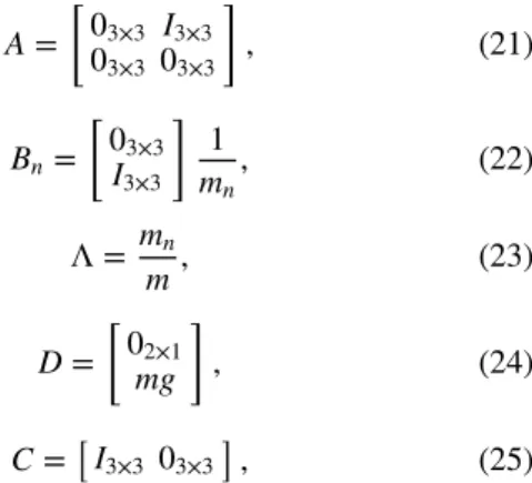
A = [ 03×3 I3×3 03×3 03×3 ] , (21) Bn= [ 03×3 I3×3 ] 1 mn, (22) Λ = mn m, (23) D = [ 02×1 mg ] , (24) C =[I3×3 03×3 ] , (25)

where m is the actual mass of the UAV that is assumed to be unknown, mnis the nominal mass, g is the gravitational accel-eration, and𝛬 represents the uncertainty in the UAV mass. It is noted that from now on, time dependence of the param-eters will not be emphasized unless necessary and therefore “t” will be dropped from the expressions.

Remark 1. The model introduced in Equation 20 represents a simple mass being controlled via virtual control inputs acting in the direction of 3 axes of the world frame in the presence of gravity, lift and drag forces, and unknown and bounded time-varying disturbances. It is noted that this representation would be accurate if the inner loop controller, which controls the attitude of the UAV, had infinite bandwidth, which is not the case. The errors due to the dynamics of the inner loop con-troller and their effects on the boundedness of the solutions of

FIGURE 3 Closed-loop control system block diagram. MRAC, model reference adaptive control; UAV, unmanned aerial vehicle. [Colour figure can be viewed at wileyonlinelibrary.com]

the overall cascaded closed-loop system are investigated later in the paper.

Remark 2. The lift and drag coefficients required to compute the wing forces in Equation 20, Wld, are obtained via nonlin-ear regression using the real data generated from wind-tunnel tests (see previous study38_{). In the controller design, these}

forces will be cancelled directly, and in the rest of the devel-opment, it will be assumed that this cancellation is already performed. The uncertainty occurring due to the computa-tion of these forces are incorporated into the time-varying disturbance term𝜋(t).

3.1.1 Reference model design

Consider the following control law, which is to be used for the nominal system dynamics, where 𝛬 = 1, D = Dn = [01×2mng]Tand𝜋(t) = 0:

un= KxTX + KrTr − Dn, (26) where r ∈ ℜ3_{, K}

x ∈ ℜ6×3, and Kr ∈ R3×3 are the ref-erence input (Xr, Yr, and Zr), control gain for the states, and control gain for the reference input, respectively. When Equation 26 is used for the nominal system, the nominal closed-loop dynamics is obtained, which is given below:

̇X_n = (A + BnKxT)X_n+ BnKTrr. (27) In Equation 27, Kx can be determined by any linear control design method, such as pole placement or linear quadratic regulator. Defining Am = A + BnKxT, nominal plant output is obtained as

yn= C(sI − Am)−1BnKTrr. (28) For a constant r, the steady-state plant output can be calcu-lated as

yss= −CA−1mBnKrTr. (29) Using KT

r = −(CA−1mBn)−1, it is obtained that lim

t→∞(yn− r) = 0. (30)

As a result, the reference model dynamics is determined as

̇X_m= AmX_m+ Bmr, (31) where Am= A + BnKxT, (32) and Bm= BnKTr (33) = −Bn ( CA−1mBn )−1 . (34)

3.1.2 Adaptive controller design

When uncertainties are considered in the system dynam-ics (Equation 20), the fixed controller gains introduced in

Equation 26 must be replaced with their corresponding adap-tive estimates:

uMRAC = ̂KxTX + ̂KrTr + ̂D, (35) with the adaptive laws given below that can be shown to result in a stable closed-loop system,42,43

̇̂Kx= −Γx ( XeTPBn+𝜎x||e|| ̂Kx ) , (36) ̇̂Kr = −Γr ( reTPBn+𝜎r||e|| ̂Kr ) , (37) ̇̂DT = −ΓD ( eT_PB n+𝜎D||e|| ̂D ) , (38) where e = X − Xm,𝛤x ∈ ℜ6×6, 𝛤r ∈ ℜ3×3, and𝛤D ∈ ℜ are adaptive gains,𝜎x,𝜎r, and𝜎Dare positive scalar gains of e-modification terms, and P ∈ℜ6×6is the symmetric solution of the Lyapunov equation

ATmP + PAm= −Q, (39) where Q ∈ ℜ6×6 _{is a positive definite matrix. However, it}

is noted that in this formulation, as mentioned earlier, it is assumed that the inner loop controller is perfect, and thus, no additional error terms appear in system dynamics due the transients of the inner loop. This assumption is violated in practice, and the attitude error dynamics from the inner loop will enter as additional disturbances to the dynamics provided in Equation 20. In the overall stability analysis of the cascaded control framework, it will be shown that with an additional quadratic e-modification robustifying term in one of the adap-tive laws, the boundedness of all closed-loop system signals can be shown. The resulting adaptive laws are given as

̇̂Kx= −Γx ( XeTPBn+𝜎x||e|| ̂Kx+𝛾x||e||2̂Kx ) , (40) ̇̂Kr = −Γr ( reTPBn+𝜎r||e|| ̂Kr ) , (41) ̇̂DT = −ΓD ( eT_PB n+𝜎D||e|| ̂D ) , (42)

where the term 𝛾x, used in the modified adaptive law (Equation 40), is a positive scalar. It is noted that the use of the newly added term “𝛾x||e||2̂Kx” will be clear in the overall stability analysis.

3.2 Attitude reference calculation

Using the translational part (first 3 rows) of Equations 2 to 9 and incorporating the disturbance term𝜋(t), we obtain that

m ̈X = (cΨcΘc_𝜃f− (cΦsΘcΨ+ sΦsΨ)s_𝜃f)u1+ Wx+𝜋x(t), (43)

m ̈Y = (sΨcΘc𝜃f − (cΦsΘsΨ− sΦcΨ)s𝜃f)u1+ Wy+𝜋y(t), (44)

m ̈Z = (−sΘc𝜃f − cΦcΘs𝜃f)u1+ mg + Wz+𝜋z(t), (45) where Wx, Wy, and Wz are the components of the lift-drag forces along 3 axes, which are given in Equation 14.

Similary,𝜋x,𝜋y, and𝜋zare the components of the disturbance term along these axes. It is important to note that, as stated in Remark 2, the wing forces are computable and therefore will be canceled in the controller implementation. Accordingly, the applied control inputs will be calculated as ui_MRAC − ̂Wj, where i = 1, 2, 3, j = x, y, z, and ̂W refers to the computed val-ues of the wing forces. As seen from Equations 20 and 43 to 45, these calculated control inputs will correspond to the pro-jections of the total thrust u1on the x-axis, y-axis, and z-axis: u1_MRAC− ̂Wx= (cΨcΘc_𝜃f − (cΦsΘcΨ+ sΦsΨ)s_𝜃f)u1, (46)

u2_MRAC− ̂Wy= (sΨcΘc𝜃_f − (cΦsΘsΨ− sΦcΨ)s𝜃_f)u1, (47)

u3

MRAC− ̂Wz= (−sΘc𝜃f − cΦcΘs𝜃f)u1. (48) It is important to note that the D term in Equation 20 addresses the gravitational force mg. In light of Equations 14 and 15, it is clear that Wx, Wy, and Wz(and therefore their computed values) are dependent on the attitude of the vehicle, ie,

[_W x Wy Wz ] = Rbw ⎡ ⎢ ⎢ ⎣ F1 D+ F 2 D+ F 3 D+ F 4 D 0 F1 L+ F 2 L+ F 3 L+ F 4 L ⎤ ⎥ ⎥ ⎦, (49)

where the lift and drag forces, F_Li and Fi_D, are given in Equation 15.

The total thrust u1 and the desired attitude angles Φdand Θdcan be found using Equations 46 to 48 as

u1= √( u1 MRAC− ̂Wx )2 +(u2 MRAC− ̂Wy )2 +(u3 MRAC− ̂Wz )2 , (50) Φd = arcsin ( −𝜌1 u1s_𝜃f ) , (51) Θd = arcsin ⎛ ⎜ ⎜ ⎝ −(u3 MRAC− ̂Wz ) u1c𝜃f − u1𝜌2s𝜃fcΦd (𝜌2)2₊(_u3 MRAC− ̂Wz )2 ⎞ ⎟ ⎟ ⎠ , (52) where 𝜌1=(u1_MRAC− ̂Wx ) sΨ_d−(u2_MRAC− ̂Wy ) cΨ_d, (53) 𝜌2=(u1_MRAC− ̂Wx ) cΨd+ ( u2_MRAC− ̂Wy ) sΨd. (54) One may obtain singular or degenerate configurations for cer-tain Φ and Θ values, since both sides of Equations 46 to 48 are functions of the vehicle attitude due to the existence of lift and drag force terms. Since the flight trajectory of the vehi-cle in this study necessitates a VTOL motion followed by a transition to horizontal flight and then back to VTOL mode for landing, throughout the study and simulations, the solu-tions given by Equasolu-tions 50 to 52 is used to calculate the total thrust and desired attitude angles. In addition, in simulation studies, we used hard limits for the desired attitude angles to

prevent feeding excessively large angles as references to the inner control loop. We leave the singular or degenerate con-figurations for which Φdand Θdcan not be obtained uniquely as a future work.

It is noted that, different from similar works in the liter-ature, the desired attitude angles are functions of the wing angles. The desired yaw angle, Ψd, can be chosen by the UAV operator that would be appropriate for the mission at hand. These required attitude angles are given to the lower-level atti-tude controller as references. The nonlinear adaptive attiatti-tude controller is described in the next section.

3.3 Nonlinear adaptive control design

To force the UAV to follow the requested attitude angles, in the presence of uncertainties, we used a nonlinear adap-tive controller similar to 1 study.44

Defining u′ = ETMt, Equation 17 can be rewritten as

M(𝛼w) ̇Ωw+ C(𝛼w, Ωw)Ωw= u′. (55) Equation 55, which describes the rotational dynamics of the vehicle, can be parameterized in a way such that the vector consisting of the diagonal elements of the moment of inertia of the UAV, IUAV= [Ixx, Iyy, Izz]T, appears linearly. This trans-formation is needed so that the uncertain moment of inertia terms appears in a form that is suitable for the adaptive control design:

Y(𝛼w, ̇𝛼w, ̈𝛼w)IUAV = u′. (56) Consider the following definition

s = ̇̃𝛼w+ Λs̃𝛼w, (57) wherẽ𝛼w=𝛼w−𝛼wd,𝛼wdis the desired value of𝛼wand𝛬s∈ ℜ3×3_{is a symmetric positive definite matrix. Equation 57 can}

be modified as

s = ̇𝛼w− ̇𝛼wr, (58)

where

̇𝛼wr= ̇𝛼wd− Λs̃𝛼w. (59) A matrix Y′= Y′(𝛼w, ̇𝛼w, ̇𝛼wr, ̈𝛼wr) can be defined, to be used in linear parameterization of Equation 55, as in the case of Equation 56, such that

M(𝛼w)̈𝛼wr+ C(𝛼w, Ωw)̇𝛼r = Y′(𝛼w, ̇𝛼w, ̇𝛼wr, ̈𝛼wr)IUAV. (60) It can be shown that the following nonlinear controller,

uNadp≡ u′= Y′ÎUAV− KDs, (61) where KD ∈ ℜ3×3 is positive definite matrix and ÎUAV is an estimate of the uncertain parameter I, with an adaptive law

̇

ÎUAV = −ΓIY′Ts, (62) where 𝛤I is the adaptation rate, stabilizes the rotational closed-loop system, and makes the error̃𝛼wconverge to 0.

The total thrust u1is provided in Equation 50. The rest of

the control inputs in Equation 9 can be calculated as in the previous study37 _{by first defining u}′′ ₌ (_E(𝛼

w)T )−1

u′ _and

performing the following operations:

u3= u ′′ 2 s_𝜃f, (63) [ u2 u4 ] = [ s_𝜃f −c_𝜃f c_𝜃f s_𝜃f ]−1[ u′₁′ u′₃′ ] . (64)

Once these control inputs are determined, the thrusts created by the rotors can be calculated using linear relationships given in Equations 10 to 13.

Remark 3. The required translational and rotational states of the UAV can be obtained by the help of several onboard sensors, such as Global Positioning System (GPS) antennas and receivers and Inertial Measurement Unit (IMU) units, processors, and algorithms, which form a full GPS Inertial Navigation System. It is noted that no state observer that needs exact plant dynamics is assumed to be available for the development of the proposed control algorithm. The infor-mation about the details of the UAV state measurements and estimation can be obtained from the literature.45

3.4 Overall closed-loop stability

In this section, the stability of the tilt-wing UAV together with the nonlinear hierarchical adaptive controller is investi-gated. Before starting this investigation, system dynamics is converted to a more suitable form for stability analysis, below. Consider the closed-loop dynamics given in Equation 20, where it is assumed that the UAV is a simple mass and is controlled via the control input uMRACin the presence of para-metric uncertainty, lift and drag forces, gravity, and unknown external disturbances. (Note that in the implementation, the computed lift and drag forces are canceled in the control sig-nal and the uncertainty in this computation is incorporated in the disturbance term, as stated in Remark 2.) Adaptive con-trol input uMRACis designed based on this assumption. This assumption is valid except that the realization of uMRAC is imperfect: The inner loop controller is used to achieve the nec-essary attitude angles that would result in the realization of

uMRAC, and since the inner loop controller does not have infi-nite bandwidth, uMRACis realized with certain errors. Specif-ically, introducing attitude-tracking errors in Equation 46 to 48, the realization of uMRACis given as

u1_MRAC =(cΨ_d+eΨcΘd+eΘcΘf− ( cΦ_d+eΦsΘd+eΘcΨd+eΨ+ sΦd+eΦsΨd+eΨ ) s𝜃f ) u1, (65) u2_MRAC =(sΨd+eΨcΘd+eΘc𝜃f −(cΦd+eΦsΘd+eΘsΨd+eΨ− sΦd+eΦcΨd+eΨ ) s_𝜃f)u1, (66) u3 MRAC= (−sΘd+eΘc𝜃f − cΦd+eΦcΘ+eΘs𝜃f)u1, (67)

where Φd, Θd, and Ψdare the desired attitude angles and eΦ, eΘ, and eΨare the attitude errors. It is noted that there is no

error term introduced to u1since the calculated desired thrust

is directly used without further realization by the inner loop controller.

Consider the following trigonometric relationships:

sin(a + b) = sin(a) + sin(b∕2)cos(a + b∕2),

cos(a + b) = cos(a) − sin(b∕2)sin(a + b∕2). (68)

Using Equation 68 and following the same procedure given in another study,46_{Equations 65 to 67 can be rewritten as}

u1_MRAC = (cΨdcΘdc𝜃f − (cΦdsΘdcΨd+ sΦdsΨd)s𝜃f + g1(Φd, Θd, Ψd, eΦ, eΘ, eΨ, 𝜃f))u1

= u1_Md+ u1g1(.),

(69)

u2_MRAC= (sΨdcΘdc𝜃f − (cΦdsΘdsΨd− sΦdcΨd)s𝜃f + g2(Φd, Θd, Ψd, eΦ, eΘ, eΨ, 𝜃f))u1

= u2_Md+ u1g2(.),

(70)

u3_MRAC = (−sΘdc𝜃f − cΦdcΘds𝜃f + g3(Φd, Θd, eΦ, eΘ, 𝜃f))u1 = u3_Md+ u1g3(.),

(71) where the terms ui_Md, i = 1, 2, and3, refer to the ith desired MRAC control input and the terms u1gi(.) are the errors, which consist of sine and cosine functions of the desired attitude angles, attitude errors, and the front wing angle, in the realization of the control inputs. Defining ud_MRAC = [u1 Md u 2 Md u 3 Md]

T _{and using Equations 69 to 71, and noting} that the total thrust u1is equal to||ud_MRAC||, Equation 20 can

be rewritten as

̇X = AX + BnΛ (

ud_MRAC+||ud_MRAC|| [ g1(.) g2(.) g3(.) ] + D +𝜋(t) ) . (72) The following lemma, regarding an upper bound on||ud

MRAC||, will be useful in providing a proof for the main theorem of this paper.

Lemma 1. For a bounded reference r,||ud_MRAC|| ⩽ c1 + c2||e|| + c3|| ̃Kx|| + || ̃Kx||||e|| + c4|| ̃Kr|| + || ̃D||, where ci are positive scalars, e ∈ ℜ6 _{is the error vector between the}

reference model states and the system states, and

̃ Kx= ̂Kx− K∗x, ̃ Kr= ̂Kr− Kr∗, ̃D = ̂D − D∗_, (73)

with (.)* _{being the “ideal value” and ̂(.) being the estimated}

value of a parameter.

It is noted that here and in the rest of the paper, Frobenius norm is used.

Remark 4. As explained earlier, the control signal given in Equation 35 is the desired control input provided by the posi-tion controller. Since in the controller development, it was assumed that this signal is realized perfectly; the superscript “d” was not used. In the stability proof, however, the position control input is represented with ud

MRAC, which removes this assumption.

Proof. (Proof of lemma 1)

Using Equation 73, Equation 35 can be rewritten as

ud_MRAC= Kx∗TX + ̃KxX + K∗

T

r r + ̃Krr + D∗+ ̃D. (74) Using the fact that e=X − Xm, Equation 74 can be rewritten as

ud_MRAC= Kx∗TXm+ K∗ T x e + ̃KxXm+ ̃Kxe + K∗ T r r + ̃Krr + D∗+ ̃D. (75) Taking the norm of both sides of Equation 75 and using the triangular inequality, it is obtained that

||ud MRAC|| ⩽ ||K ∗T x ||||Xm|| + ||K∗ T x ||||e|| + || ̃Kx||||Xm|| +|| ̃Kx||||e|| + ||K∗ T r ||||r|| + || ̃Kr||||r|| +||D∗_{|| + || ̃D||.} (76) K∗

x, K∗r, and D*are constant matrices. Also, it is known that the states of the reference model Xmare bounded. Defining ||K∗

x|| ≡ k1,||Kr∗|| ≡ k2,||D*|| ≡ k3,||r|| ≡ k4, and||Xm|| ≡

k5, Equation 76 can be rewritten as ||ud

MRAC|| ⩽ k1k5+ k1||e|| + k5|| ̃Kx|| + || ̃Kx||||e|| + k2k4 + k4|| ̃Kr|| + k3+|| ̃D||. (77) Defining c1≡ k1k5+ k2k4+ k3, c2 ≡ k1, c3≡ k5, and c4≡ k4, it is obtained that ||ud MRAC|| ⩽ c1+c2||e||+c3|| % K x||+|| % K x||||e||+c4|| % K r||+|| % D||. (78) This completes the proof of Lemma 1.

The following lemma will also be instrumental in proving the main theorem of this work.

Lemma 2. ̄G ⩽ k||̃𝛼_𝜔||, where ̃𝛼_𝜔 is the attitude-tracking error vector and k is a positive constant.

Remark 5. A classical hierarchical controller is designed in previous study36 _{for a similar plant, where the errors}

intro-duced by the inner loop controller is investigated. It is noted that regardless of the controller type, the same error terms will appear as disturbances in the outer loop controller. A proof of Lemma 2 is given in another study,36_{and thus, the proof is}

omitted here.

Theorem 1. All the signals in the closed-loop system, con-sisting of the UAV dynamics (Equation 72), the reference model (Equation 31), MRAC (Equations 35-42), and nonlin-ear adaptive controller (Equations 61 and 62), are uniformly ultimately bounded (UUB), which indicates that the bound on the signals does not depend on the initial time t0 and

that this uniform bound holds after a certain time T, ie, for t ⩾ t0 + T. It is noted that in UUB, unlike Lyapunov

sta-bility, the bound on the signals cannot be made arbitrarily small with proper initial conditions. In practice, this bound is a function of uncertainties and disturbances.42_{In addition,}

defining G(.) = [g1(.)g2(.)g3(.)]T, the following are true: lim

t_→∞G(.) = 0, (79)

sup||G(.)|| ⩽ k||Λ−1s ||

×((K −𝜆min(Γ−1) ×||̃IUAV||2 )

∕ ̄𝜆max(M) )1∕2

,

(80) where 0 ∈ℜ3_{is a vector of zeros, k ∈ℜ}+_{is a constant, “sup”}

refers to “supremum,” ̄𝜆max is the bound on the maximum eigenvalue of M, and

K = 1

2 (

s(0)TM(0)s(0) + ̃IUAV(0)TΓ−1I ̃IUAV(0) )

. (81)

Proof. (Proof of Theorem 1:)

In light of Remark 4, substituting the control input Equation 35 into Equation 72, it is obtained that

̇X = (A + BnΛ ̂KTx ) X + BnΛ ( ̂KT rr + ̂D +||ud_MRAC|| [_g1(.) g2(.) g3(.) ] + D +𝜋(t) ) . (82) Assuming that there exist K∗

x and Kr∗such that

A + BnΛK∗ T x = Am, BnΛK∗ T r = Bm, (83)

and defining ̂Kx= Kx∗+ ̃Kx, ̂Kr = Kr∗+ ̃Krand ̂D = D∗+ ̃D = −D + ̃D, Equation 82 can be rewritten as

̇X = AmX + Bmr + BnΛ ̃KxTX + BnΛ ̃KrTr + BnΛ ̃D + BnΛ||ud_MRAC|| [_g 1(.) g2(.) g3(.) ] + BnΛ𝜋(t). (84)

Subtracting the reference model Equation 31 from Equation 84, it is obtained that

̇e = Ame + BnΛ ̃KxTX + BnΛ ̃KrTr + BnΛ ̃D + BnΛ||ud_MRAC|| [_g1(.) g2(.) g3(.) ] + BnΛ𝜋(t), (85) where e = X − Xm.

Consider the following Lyapunov function candidate

V = eTPe + tr([ ̃KxTΓ−1x ̃Kx+ ̃KrTΓ−1r ̃Kr+ ̃DTΓ−1_D ̃D] Λ) , (86) where “tr” refers to the trace operation and P is a symmetric positive definite matrix that is the solution of the Lyapunov equation

ATmP + PAm= −Q, (87)

where Q ∈ℜ6×6_{is a symmetric positive definite matrix.}

Tak-ing the derivative of both sides of Equation 86, it is obtained that ̇V = ̇eT Pe + eTṖe + 2tr ([ ̃KT xΓ−1x ̇̃Kx+ ̃KrTΓ−1r ̇̃Kr+ ̃DTΓ−1_D ̇̃D ] Λ ) =(eTATm+ XT̃KxΛBnT+ rT̃KrΛBTn + ̃DTΛBTn +G(.)T||ud_MRAC||ΛBTn+𝜋(t)TΛBTn ) Pe + eTP(Ame + BnΛ ̃KxTX + BnΛ ̃KrTr + BnΛ ̃D +BnΛ||ud_MRAC||G(.) + BnΛ𝜋(t) ) + 2tr([̃KxTΓ−1x ̇̃Kx+ ̃KrTΓ−1r ̇̃Kr+ ̃DTΓ−1_D ̇̃D ] Λ) = eT(ATmP + PAm ) e + 2eTPBnΛ( ̃KxTX + ̃KrTr + ̃D +||ud_MRAC||G(.) + 𝜋(t)) + 2tr([̃KxTΓ−1x ̇̃Kx+ ̃KrTΓ−1r ̇̃Kr+ ̃DTΓ−1D ̇̃D ] Λ) = −eTQe + 2eTPBnΛ ̃KxTX + 2tr ([ ̃KT xΓ−1x ̇̃Kx ] Λ) + 2eTPBnΛ ̃KrTr + 2tr ([ ̃KT rΓ−1r ̇̃Kr ] Λ ) + 2eTPBnΛ ̃D + 2tr([̃DT_Γ−1 D ̇̃D ] Λ)+ 2eT_PB nΛ||ud_MRAC||G(.) + 2eTPBnΛ𝜋(t), (88) where G(.) = [g1(.)g2(.)g3(.)]T_{. Using the property of the} trace operator, aT_{b = tr(ba}T_{), where a and b are vectors,} Equation 88 can be rewritten as

̇V = −eT Qe + 2tr([̃KxTΓ−1x ̇̃Kx+ ̃KxTXeTPBn ] Λ) + 2tr([̃KrTΓ−1r ̇̃Kr+ ̃KrTreTPBn ] Λ) + 2tr ([ ̃DT Γ−1_D ̇̃D + ̃DTeTPBn ] Λ ) + 2eTPBnΛ||ud_MRAC||G(.) + 2eTPBnΛ𝜋(t). (89)

Substituting Equations 40 to 42 in Equation 89, it is obtained that ̇V = −eT Qe + 2tr([−𝜎x̃KxT||e|| ̂Kx−𝛾x̃KTx||e||2̂Kx ] Λ) + 2tr(−𝜎r̃KrT||e|| ̂KrΛ ) + 2tr(−𝜎D̃DT||e|| ̂DΛ ) + 2eTPBnΛ||ud_MRAC||G(.) + 2eTPBnΛ𝜋(t) ⩽ −||e||2_𝜆 min(Q) + 2 tr ([ −𝜎x̃KxT||e|| ̂Kx−𝛾x̃KxT||e||2̂Kx −𝜎r̃KrT||e|| ̂Kr−𝜎D̃DT||e|| ̂D ] Λ)

+ 2||e||||PBnΛ||||ud_MRAC||||G(.)|| + 2||e||||PBnΛ|| ̄𝜋, (90) where𝜆min(Q) refers to the minimum eigenvalue of the matrix

Q and ̄𝜋 is the upper bound of 𝜋(t). Using the fact that

the norm of the vector G(.) is bounded by a constant ̄G,

since the vector terms consist of sines and cosines, and using Lemma 1, it is obtained from Equation 90 that

̇V ⩽ −||e||2_𝜆 min(Q) + 2 tr ([ −𝜎x̃KxT||e|| ̂Kx−𝛾x̃KxT||e||2̂Kx −𝜎r̃KrT||e|| ̂Kr−𝜎D̃DT||e|| ̂D ] Λ) + 2 ̄G||e||||PBnΛ|| ( c1+ c2||e|| + c3|| ̃Kx|| + || ̃Kx||||e|| +c4|| ̃Kr|| + || ̃D|| ) + 2||e||||PBnΛ|| ̄𝜋. (91) Completing the square, the first term in the trace operation parenthesis can be rewritten as follows:

tr([−𝜎x̃KTx||e|| ̂Kx ] Λ)⩽ 𝜆min(Λ) × tr ( −𝜎x̃KxT||e|| ( Kx∗+ ̃Kx )) = −𝜎x||e||𝜆min(Λ) ( K∗ x 2 + ̃Kx 2 − K ∗ x 2 2) ⩽ −𝜎x||e||𝜆min(Λ) ( ̃Kx 2 − Kx∗2 ) . (92) Using the same procedure, Equation 91 can be rewritten as

̇V ⩽ −||e||2_𝜆

min(Q) −𝜎x||e||𝜆min(Λ) ̃Kx

2 +𝜎x||e||𝜆min(Λ) Kx∗2 −𝛾x||e||2𝜆min(Λ) ̃Kx 2 +𝛾x||e||2𝜆min(Λ) Kx∗2 −𝜎r||e||𝜆min(Λ) ̃Kr 2 +𝜎r||e||𝜆min(Λ) Kr∗2 −𝜎D||e||𝜆min(Λ) ̃D 2 +𝜎D||e||𝜆min(Λ) D∗ 2 + 2 ̄G||e||||PBnΛ|| ( c1+ c2||e|| + c3|| ̃Kx|| + || ̃Kx||||e|| +c4|| ̃Kr|| + || ̃D|| ) + 2||e||||PBnΛ|| ̄𝜋 = −||e||(||e||{𝜆min(Q) +𝛾x𝜆min(Λ) ̃Kx2 −𝛾x𝜆min(Λ) Kx∗2− 2 ̄G||PBnΛ|||| ̃Kx|| − 2 ̄G||PBnΛ||c2 } +𝜎x𝜆min(Λ) ̃Kx 2 −𝜎x𝜆min(Λ) Kx∗2 +𝜎r𝜆min(Λ) ̃Kr 2 −𝜎r𝜆min(Λ) Kr∗2+𝜎D𝜆min(Λ) ̃D 2 −𝜎D𝜆min(Λ) D∗ 2− 2 ̄G||PBnΛ||c1 − 2 ̄G||PBnΛ||c3|| ̃Kx|| − 2 ̄G||PBnΛ||c4|| ̃Kr|| − 2 ̄G||PBnΛ|||| ̃D|| − 2||PBnΛ|| ̄𝜋 ) . (93) Assume that there exists an𝜀 > 0 such that

𝜆min(Q) +𝛾x𝜆min(Λ) ̃Kx

2

−𝛾x𝜆min(Λ) Kx∗2− 2 ̄G||PBnΛ|||| ̃Kx|| − 2 ̄G||PBnΛ||c2−𝜀 > 0.

(94) Using Equation 94, it can be concluded that ̇V ⩽ 0 in the complement of the set S, where S is defined as

S≡{ (e, ̃Kx, ̃Kr) ||𝜀||e|| + 𝜎x𝜆min(Λ) ̃Kx2 −𝜎x𝜆min(Λ) Kx∗2+𝜎r𝜆min(Λ) ̃Kr 2 −𝜎r𝜆min(Λ) Kr∗2+𝜎D𝜆min(Λ) ̃D 2 −𝜎D𝜆min(Λ) D∗ 2− 2 ̄G||PBnΛ||c1 − 2 ̄G||PBnΛ||c3|| ̃Kx|| − 2 ̄G||PBnΛ||c4|| ̃Kr|| − 2 ̄G||PBnΛ|||| ̃D|| − 2||PBnΛ|| ̄𝜋 ⩽ 0 } . (95)

Therefore, using standard arguments, it can be shown43_that

all the solutions are UBB. This completes the proof of the first part of Theorem 1. It is noted that the inclusion of the quadratic e-modification robustifying term in Equation 40 is beneficial in obtaining a negative semidefinite Lyapunov function derivative.

It is noted that the assumed system property (Equation 94) can be investigated further by completing the square and rewriting the inequality as

𝜆min(Q) + ( √ 𝛾x𝜆min(Λ) ̃Kx − ̄G||PB nΛ|| √ 𝛾x𝜆min(Λ) )2 −𝛾x𝜆min(Λ) Kx∗2− ̄G2_||PB nΛ||2 𝛾x𝜆min(Λ) − 2 ̄G||PBnΛ||c2−𝜀 > 0. (96)

A sufficient condition to satisfy this inequality is given as

𝜆min(Q) −𝛾x𝜆min(Λ) Kx∗2> ̄G2_||PB nΛ||2 𝛾x𝜆min(Λ) + 2 ̄G||PBnΛ||c2+𝜀. (97)

Remark 6. Both the bound on the tracking error in Equation 95 and the restriction on system parameters given in Equation 97 are directly related to the size of the param-eter ̄G, which is an upper bound for the vector G(.), which

consists of elements that are sine and cosine functions of the attitude-tracking errors. These elements were introduced in Equation 69 to 71. In the above development, a conservative approach is taken about this upper bound by simply stating that since these vector elements are sine and cosine func-tions of the attitude errors, the vector norm has to be bounded by some constant ̄G. Below, in the second and third parts of

the proof, the vector G(.) is investigated further to show that (1) limt→∞G(.) = 0, (2) the supremum norm of the vector

G(.) can be made arbitrarily small by choosing the

nonlin-ear adaptive controller constant𝛬slarge enough. In practice, this choice of𝛬sis limited by the high-frequency unmodeled dynamics of the system together with measurement noise.47

From the first part of Theorem 1, which is proven above, it is known that the states X,Y, Z, and the adaptive param-eter errors ̃Kx, ̃Kr, and ̃D are bounded. Therefore, for a bounded reference r, the control input (Equation 35) is bounded. This implies that the total thrust u1 determined

in Equation 50 is bounded, which shows that the desired attitude angles Φd and Θd, calculated in Equations 51 and 52, which are passed to the inner loop controller as refer-ence inputs, are also bounded. Therefore, the attitude control loop, explained in subsection 3.3 can be shown to be asymp-totically stable,47 _{meaning that the attitude-tracking error}

̃𝛼𝜔 = [(Φd− Φ) (Θd− Θ) (Ψd− Ψ)]T converges to zero asymptotically. Once this is established, it is straightforward to see that limt→∞G(t) = 0 ∈ ℜ3. This completes the proof of the second part of Theorem 1.

It can be shown that the derivative of the following Lya-punov function,

V1(t) = 1 2 [

sTMs + ̃IUAVΓ−1_I ̃IUAV ]

, (98)

is negative semidefinite.47_{This implies that}

1 2 [

s(t)TM(t)s(t) + ̃IUAV(t)Γ−1I ̃IUAV(t) ] ⩽ 1

2 (

s(0)T_{M(0)s(0) + ̃I}

UAV(0)TΓ−1_I ̃IUAV(0) )

, ∀t ⩾ 0.

(99) After some manipulation, it is obtained from Equation 100 that

1 2 [

s(t)TM(t)s(t) + ̃IUAV(t)Γ−1I ̃IUAV(t) ] ⩽ 1

2 (

s(0)T_{M(0)s(0) + ̃I}

UAV(0)TΓ−1_I ̃IUAV(0) )

, ∀t ⩾ 0.

(100) After some manipulation, it is obtained from Equation 100 that

||s(t)|| ⩽((K −𝜆min(Γ−1I )||̃IUAV||2 ) ∕ ̄𝜆max(M) )1∕2 , (101) where K = 1 2 (

s(0)TM(0)s(0) + ̃IUAV(0)TΓ−1_I ̃IUAV(0) )

. (102) From the definition of s given in Equation 57, it is obtained that

||̃𝛼𝜔|| ⩽ ||s(t)|| Λ−1s (I − e−tΛs) ⩽ ||s(t)|| Λ−1s . (103) Using Lemma 2 and Equations 101 and 103, it is straightfor-ward to prove the third part of Theorem 1. This completes the proof of the third part of Theorem 1.

Remark 7. The implication of Equation 79 is that the “distur-bance” [g1(.)g2(.)g3(.)]Tintroduced to the closed-loop system

(Equation 82), because of the dynamics of the attitude con-trol loop, converges to zero. The speed of convergence is determined by the selection of the nonlinear adaptive con-trol parameters. For all practical purposes, the convergence of the disturbance to zero means that the origin remains to be an equilibrium point of the proposed closed-loop control sys-tem structure even though robustfiying terms are used in the adaptive control laws (Equations 36-38).

Remark 8. The implication of Equation 80 is that the suf-ficiency condition (Equation 97) is not too restrictive since

̄G can be made small with a large enough 𝛬s. As mentioned earlier, the size of𝛬s is limited by measurement noise and unmodeled high frequency dynamics.

4 I M P L E M E N T A T I O N S C E N A R I O

To examine the behavior of the tilt-wing UAV, during takeoff (quadrotor mode), horizontal flight (fixed wing mode), and transitions between these modes, we created a flight scenario as shown in Figure 4. The UAV takes off

vertically with 90◦ wing angles (0-10 seconds), and after reaching a desired altitude, it changes its wing angles to 20◦ (10-20 seconds). After flying in horizontal mode for about 650 m (20-65 seconds), it changes its wing angles back to 90◦, while slowing down (65-100 seconds). Then, it lands as a quadrotor (100-110 seconds). It is noted that during

level flight, at t = 61 seconds, 2 batteries, wing covers and winglets, fall, all from the right wing. Furthermore, Dryden wind gust model48 _{is used to create external disturbances.}

Below, the changes in mass, moment of inertia, and center of gravity are investigated because of wing movements and failures. Also, a trajectory generation method is given.

FIGURE 4 Flight scenario. [Colour figure can be viewed at wileyonlinelibrary.com]

FIGURE 5 Inertia variations during transition from quadrotor mode to fixed-wing mode, before the failure. [Colour figure can be viewed at wileyonlinelibrary.com]

Remark 9. The above trajectory description also explains the proposed method for the transitions between quadrotor and fixed-wing modes: After a vertical takeoff with 90◦wing angles, the first transition occurs from the quadrotor mode to fixed-wing mode, where the altitude is kept fixed and wing angles are moved from 90◦to 20◦. During this transition, the aircraft pitch angle increases to prevent the loss of the lift force. After the wings obtain 20◦angle, the aircraft moves for-ward horizontally as a fixed-wing aircraft causing the pitch angle to go back to 0◦. As the aircraft gets closer to the tar-get destination, wings start to move from 20◦angle to 90◦and the aircraft starts to slow down until it comes to a full stop in the air while keeping the altitude constant. When the aircraft stops its horizontal movement, the wing angles reach 90◦and then the aircraft, now in the quadrotor mode, lands on the ground vertically. The pitch and wing-angle variations during these transitions can be seen more clearly in the simulation results in Section 5.

4.1 Moment of inertia variations during transition stages

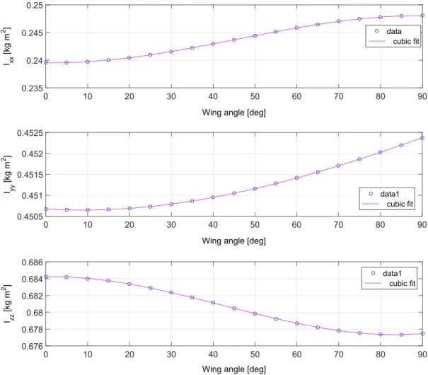
The vehicle’s computer-aided design model generated in SolidWorks was used to extract the principal moment of inertia changes during the transition. For the transition from

quadrotor mode to fixed-wing mode, wing angles were changed from 90◦to 0◦with 5◦intervals, and for each interval, principal moment of inertias was calculated in SolidWorks. Then, cubic polynomials are used for curve fitting. The result-ing curves can be seen in Figure 5.

The same procedure is used to calculate the variations in the moment of inertias during the transition from the fixed-wing mode to quadrotor mode. However, during this transition, the UAV model is different than the one in the first transition because of the missing parts that are lost at the moment of failure at t = 61 seconds. The resulting curves are presented in Figure 6.

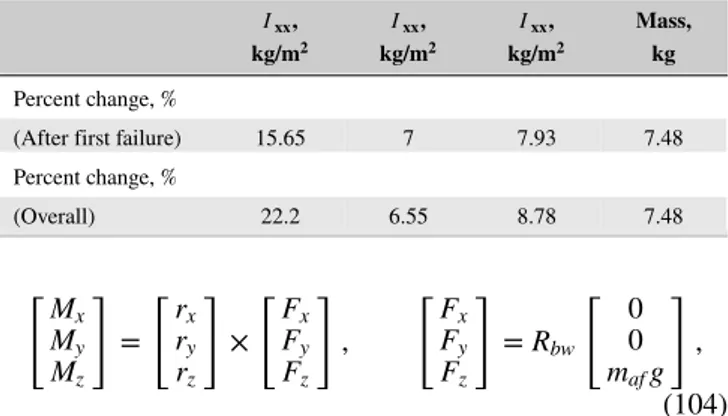
In the simulations, these curves were used to obtain the parameter changes during the transition stages and during the failure. Percent changes in these system parameters are presented in Table 1.

4.2 Center of gravity variation due to the failure

In addition to moment of inertia and mass changes, center of gravity of UAV changes with the failure. This change is modeled as an external disturbance to UAV position dynam-ics, which consists of the moments Mx, My, and Mz that are calculated as

FIGURE 6 Inertia variations during transition from fixed-wing mode to quadrotor mode, after the failure. [Colour figure can be viewed at wileyonlinelibrary. com]

TABLE 1 Percent changes of principal moment of inertias and mass

Ixx, Ixx, Ixx, Mass,

kg/m2 _kg/m2 _kg/m2 _kg

Percent change, %

(After first failure) 15.65 7 7.93 7.48

Percent change, % (Overall) 22.2 6.55 8.78 7.48 [_M x My Mz ] = [_r x ry rz ] × [_F x Fy Fz ] , [_F x Fy Fz ] = Rbw [ ₀ 0 mafg ] , (104) where Rbwis the rotation matrix that gives orientation of the body frame with respect to the world frame, g is the grav-itational accelaration, maf is the mass of the UAV after the failure, and rx, ry, and rz are distances of the center of grav-ity to the original position before the failure, measured along the axes.

4.3 Trajectory generation

4.3.1 Forward velocity determination

Tilt-wing UAV tilts its wings during long-duration flights to benefit from the lift forces and flies like a fixed-wing UAV as presented in Figure 1, right picture. However, position ref-erence along the x-axis of world coordinate frame may force the vehicle to fly with relatively slow velocities, which results in a dramatic increase at the pitch angle. Therefore, a min-imum forward velocity should be identified that results in a reduced pitch angle during horizontal flight. In this study, a zero-degree pitch angle is targeted.

To obtain the minimum forward velocity that will lead to a zero-degree pitch angle during horizontal flight, we recalled the aerial vehicle position dynamics along the z-axis:

̈Z = 1 m

[

(−s_𝜃c_𝜃f − c_𝜑c_𝜃s_𝜃f)u1+ mg + Wz],

where sine and cosine of the angles are denoted by s and c, respectively. There should be a zero net force along the z-axis (ie, m ̈Z = 0) for a level flight. Additionally, pitch angle should be set to zero, which results in

c𝜑s𝜃fu1− mg = Wz. (105) Aerodynamic forces along x-axis, y-axis, and z-axis of the world coordinate frame can be defined as

W(𝜁) = [Wx, Wy, Wz]T = ⎡ ⎢ ⎢ ⎣ Rwb ⎡ ⎢ ⎢ ⎣ 2((Ff_D(𝜃f, vx, vz) + Fr_D(𝜃r, vx, vz)) 0 2((F_Lf(𝜃f, vx, vz) + Fr_L(𝜃r, vx, vz)) ⎤ ⎥ ⎥ ⎦ ⎤ ⎥ ⎥ ⎦ , (106) where Rwb is the rotation matrix between world and body frame and Fi_L(𝜃f, vx, vz) and Fi_D(𝜃f, vx, vz) are the lift and drag forces produced by the wings (i = f, r subscripts denote front and rear angles, respectively). To simplify the analysis,

front and rear wing angles assumed to be equal (𝜃f = 𝜃r). Therefore, lift and drag forces are defined as

Ff_L(𝜃f, vx, vz) = Fr_L(𝜃r, vx, vz) = FL,

F_Df(𝜃f, vx, vz) = Fr_D(𝜃r, vx, vz) = FD. From Equation 106, wing forces along z-axis becomes

Wz= −s𝜃(4FD) + c𝜑c𝜃(4FL). If the pitch angle is zero, then Wzbecomes

Wz= c𝜑(4FL).

Substituting Wzin Equation 105, the lift force that is necessary for a level flight can be found as

FL=

c_𝜑s_𝜃fu1− mg

4c𝜑 . (107)

The lift and drag forces are given as ⎡ ⎢ ⎢ ⎣ Fi_D 0 Fi L ⎤ ⎥ ⎥ ⎦ = R(𝜃i−𝛼i) ⎡ ⎢ ⎢ ⎣ 1 2CD(𝛼i)𝜌Av 2 𝛼 0 1 2CL(𝛼i)𝜌Av 2 𝛼 ⎤ ⎥ ⎥ ⎦, (108)

where𝜌 is the air density, A is the wing planform area, and

R(𝜃i−𝛼i) is the rotation matrix for the rotation around y-axis that decomposes the forces on the wings onto the body axes. Defining𝛽 = 𝜃i−𝛼i, R(𝛽) becomes R(𝛽) = [ _c 𝛽 0 s𝛽 0 1 0 −s_𝛽 0 c_𝛽 ] . v_𝛼is the airstream velocity, which is defined as

v_𝛼= √

v2

x+ v2z, (109)

where vxand vzare UAV’s velocities along x-axis and y-axis of the body coordinate frame. 𝛼i is the effective angle of attack, which is defined as𝛼i = 𝜃i− (−atan(vz, vx)). Using Equations 107 and 108, it is obtained that

−2s_𝛽CD𝜌Av2_𝛼+ 2c_𝛽CL𝜌Av2_𝛼=

c_𝜑s_𝜃fu1− mg

c_𝜑 . (110)

The minimum forward velocity in the body coordinate frame that can achieve zero-degree pitch angle is obtained using Equations 109 and 110 as vx= √ c_𝜑s_𝜃fu1− mg 2c_𝛽c_𝜑CL𝜌A − 2s𝛽c𝜑CD𝜌A − v2 z. (111)

Using the transformation of linear velocities between the body and the world frames, Vw = RbwVb, minimum forward linear velocity in the world frame that can achieve zero-degree pitch angle can be identified as

FIGURE 7 X tracking. [Colour figure can be viewed at wileyonlinelibrary.com]

FIGURE 8 Y tracking. [Colour figure can be viewed at wileyonlinelibrary.com]

FIGURE 10 Φtracking. [Colour figure can be viewed at wileyonlinelibrary.com]

FIGURE 11 Θtracking. [Colour figure can be viewed at wileyonlinelibrary.com]

4.3.2 Velocity profile determination

If minimum velocity, which creates enough lift forces to sus-tain level flight of the UAV, is not achieved, UAV starts to increase its pitch angle. Therefore, a suitable trajectory is generated along the x-axis by using so-called linear segments with parabolic blends. This trajectory has a trapezoidal veloc-ity profile where a constant velocveloc-ity can be imposed between predefined time instances, as well as linear (ramp) veloc-ity variations. The resulting trajectory consists of quadratic and linear polynomials with smooth blending between them. A more detailed analysis of linear segments with parabolic blends can be found in 1 study.49

Remark 10. In this study, we chose to provide a practical approach for trajectory generation, where a horizontal flight with minimum pitch angle is required. However, there may be applications where the goal is minimizing energy consump-tion and the resultant pitch angle and speed and wing angle can be tolerated. In that case, the necessary wing angle and forward speed combination that would result in maximum lift

to drag ratio should be calculated and a suitable trajectory should be generated to achieve this combination.

5 S I M U L A T I O N R E S U L T S

In this section, the performance of the proposed adaptive con-trol framework is investigated using the scenario explained in the previous section. It is noted that all the simulations are conducted using a high-fidelity simulation model, in the pres-ence of uncertainties, disturbances, and measurement noise. In addition to the changes in the mass, moment of inertia, and center of gravity, due to the failure, a 10% uncertainty is assumed in the actuator powers. Also, a 20% actuator power loss is assumed because of the failure at t = 61 seconds where 2 batteries fall. The performance of the fixed controller used in earlier studies,37 _{which is a cascade of a PID controller}

(outer loop) and a feedback linearazition + PID controller (inner loop), is also given as a comparison. As expected, the

FIGURE 13 Control inputs. [Colour figure can be viewed at wileyonlinelibrary.com]

FIGURE 15 Wing angles. [Colour figure can be viewed at wileyonlinelibrary.com]

FIGURE 16 Wing forces. [Colour figure can be viewed at wileyonlinelibrary.com]

adaptive controller outperforms the fixed controller due to its adaptability to uncertainties.

Figures 7 to 9 show the performance of the controllers for the position trajectory tracking. The closed-loop system with the adaptive controller deviates much less from the trajectory compared with the fixed controller, especially after the failure instant at t = 61 seconds.

Figures 10 to 12 show the attitude-tracking curves. As seen from the figures, the system with the proposed controller can keep its roll (Φ) and yaw (Ψ) angles close to zero. On the other hand, UAV shows large roll and yaw-angle variations when the fixed controller is in charge. The 2 controllers are compa-rable in the variations in the pitch angle (Θ) until the failure instant, but after the failure at t = 61 seconds, the pitch angle varies more smoothly with the proposed controller compared with the fixed controller.

It is noted that although its performance is not as good as the adaptive controller, the fixed controller can still keep the closed-loop system under the influence of parametric uncertainties, center of gravity, mass and moment of inertia changes as well as actuator power losses, wind disturbances, and measurement noise. However, the fixed controller pays the price by outputting very noisy control inputs. As seen from Figure 13, especially between t = 30 − 60 seconds, the fixed controller output have high-amplitude high-frequency components. It is noted that at this time interval, the UAV’s forward speed reaches its maximum value of ≈ 50 km/h. On the other hand, the adaptive control inputs are smoother. The wind disturbances can be seen in Figure 14, where the distur-bances acting on the UAV are seen to be different at certain

time intervals for different controller implementations due to speed, orientation, and altitude differences.

Figure 15 shows the movement of the wings during the flight, and Figure 16 shows the resulting aerodynamic forces acting on the wings. It is seen that a considerable amount of lift is generated together with some drag force. For the energy gain compared to a similar quadrotor without wings to be cal-culated, it is assumed that the wingless quadrotor would need less force in the x direction due to zero drag (from the wings) and more force in the z direction due to the lack of lift. With these considerations, it is calculated that the quad tilt-wing UAV spends ≈ 33% less energy, compared with a conven-tional wingless quadrotor, for the flight scenario used in this study.

6 C O N C L U S I O N S

A nonlinear adaptive control framework that works in a hierarchical structure is proposed for the control of a quad tilt-wing UAV. The controller development does not need any linearization of the UAV dynamics. Rigorous stability analysis of the controller is provided. The controller is imple-mented using a nonlinear, high-fidelity model of the tilt-wing UAV, in the presence of uncertainties, actuator failures, struc-tural failures, center of gravity changes due to these failures, and the effect of wing-angle variations on moment of inertia. The implementation results show that the proposed controller works as intended and performs dramatically better than the fixed controller used in earlier flight tests.