Vol. 13, No. 4, 2018
dx.doi.org/10.2140/jomms.2018.13.571
msp
GROWTH-INDUCED INSTABILITIES OF AN ELASTIC FILM ON A VISCOELASTIC SUBSTRATE: ANALYTICAL SOLUTION AND COMPUTATIONAL APPROACH VIA EIGENVALUE ANALYSIS
IMANVALIZADEH, PAULSTEINMANN AND ALIJAVILI
The objective of this contribution is to study for the first time the growth-induced instabilities of an elastic film on a viscoelastic substrate using an analytical approach as well as computational simulations via eigenvalue analysis. The growth-induced instabilities of a thin film on a substrate is of particular interest in modeling living tissues such as skin, brain, and airways. The analytical solution is based on Airy’s stress function adopted to viscoelastic constitutive behavior. The computational simulations, on the other hand, are carried out using the finite deformation continuum theory accounting for growth via the multiplicative decomposition of the deformation gradient into elastic and growth parts. To capture the critical growth of elastic films and the associated folding pattern, eigenvalue analysis is utilized, in contrast to the commonly used perturbation strategy. The eigenvalue analysis provides accurate, reliable, and reproducible solutions as contrasted to the perturbation approach. The numerical results obtained from the finite element method show an excellent agreement between the computational simulations and the proposed analytical solution.
1. Introduction
Instabilities of bilayered structures consisting of a thin stiff film adhered to an infinite substrate are increasingly important due to their applications in biological tissues. Such structural instabilities in the form of wrinkles[Cao and Hutchinson 2012b;Budday et al. 2014], folds[Sun et al. 2012;Sultan and Boudaoud 2008], or creases[Cao and Hutchinson 2012a;Hong et al. 2009;Jin et al. 2015]have been studied recently. In many living systems, the formation of structural instabilities is critical to appropriate biological function of the system[Wyczalkowski et al. 2012]. Typical examples are wrinkling of skin[Tepole et al. 2011], villi formation in the intestine[Balbi and Ciarletta 2013], and folding of the developing brain[Xu et al. 2010;Budday et al. 2014;Budday and Steinmann 2018]. However, in some biological systems, the formation of structural instabilities can be an indication of a disease, e.g., the folding of the mucous membrane in asthmatic airways[Wiggs et al. 1997].
It is thus not surprising that the mathematical modeling of folding in tubular organs [Ciarletta and Ben Amar 2012], in particular the modeling of the folding mucous membrane[Moulton and Goriely 2011;Li et al. 2011;Xie et al. 2014], has attracted increasing scientific attention in the past decade. This problem (and variants thereof) has been widely studied lately[Budday et al. 2015;Cao and Hutchinson 2012b;Huang et al. 2005;Hutchinson 2013;Jin et al. 2011;Sun et al. 2012;Xu et al. 2014].
The concept of growth commonly has been modeled by continuum approaches via the multiplicative decomposition of the deformation gradient into an elastic and a growth part[Rodriguez et al. 1994]which
Keywords: growth-induced instabilities, viscoelasticity, wrinkling, finite element method. 571
pairs the growth to the kinematic level[Taber 1995]. This concept requires the introduction of an artificial intermediate configuration[Garikipati et al. 2004]. Additional details on the continuum theory of growth and its implications are discussed in [Ciarletta and Maugin 2011;Ciarletta et al. 2013;Dervaux and Ben Amar 2011;Dunlop et al. 2010;Epstein and Maugin 2000;Garikipati et al. 2004;Goriely et al. 2008;
Kuhl et al. 2003;Li et al. 2011;Yavari 2010;Ben Amar and Goriely 2005;Javili et al. 2014], amongst others. Growth is commonly formulated within the framework of open-system thermodynamics[Kuhl and Steinmann 2003;Kuhl 2014]where the body is allowed to constantly exchange mass, momentum, and entropy with its environment through corresponding fluxes across its boundary; see also[Cowin and Hegedus 1976;Epstein and Maugin 2000;Javili et al. 2013].
Most of the contributions on the subject assume the compliant substrate to be elastic. This contribution for the first time studies the growth-induced instabilities of an elastic film on a viscoelastic substrate from both analytical and computational perspectives using eigenvalue analysis and, in particular, elaborates on the role of the relaxation time on the instability pattern as well as the critical growth; see also[Huang and Suo 2002;Huang 2005;Budday et al. 2014]. Key features of this contribution are:
(1) to study the growth-induced instabilities of an elastic film on a viscoelastic substrate from both analytical and numerical perspectives,
(2) to employ the eigenvalue analysis proposed in[Javili et al. 2015]for the numerical solution and not the common perturbation strategy, and
(3) to illustrate an excellent agreement between the numerical and analytical solutions.
This manuscript is organized as follows. Section 2deals with the computational approach to study growth-induced instabilities of a thin film on a compliant viscoelastic substrate. Next, the analytical solution of the problem is derived inSection 3and its simplification to various classes of viscoelastic models are discussed. The results from the computational approach using the finite element method are compared against the analytical solution through a series of numerical examples inSection 4and it is found that the two strategies are in excellent agreement. Finally, Section 5concludes this work and provides further outlook.
2. Computational approach
The numerical solution of the problem is achieved by using the finite deformation theory in continuum mechanics to account for growth, whereby the deformation gradient is decomposed multiplicatively into an elastic and a growth part.
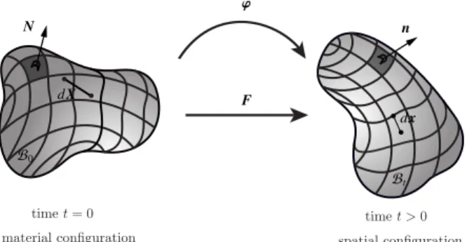
Let the continuum bodyB0occupy the material configuration at time t = 0, as shown inFigure 1. The
motion ' maps the bodyB0to the spatial configurationBt at time t. The deformation gradient F maps
the line element dx fromB0to dx inBt and is defined as F := Grad '. The governing balance equations
of finite deformation continuum mechanics consist of the balance of linear and angular momentum. The balance of linear momentum in material configuration, for bodyB0at time t = 0 and a quasistatic process,
reads
F N n dx Bt B0 dX Figure 1: kinematics
Figure 1. The material and spatial configurations of a continuum body with associated nonlinear deformation map ' and the linear tangent map F := Grad '.
where P is Piola stress1andb
0is the body force density in the material configuration. The balance of
angular momentum leads to the symmetry of the Cauchy stress tensor = trelated to the Piola stress
via P = · Cof F.
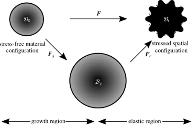
2.1. Growing elastic film. To model volumetric growth one can use the multiplicative decomposition of the deformation gradient F into a growth part Fg and an elastic part Fe as
F = Fe· Fg) Fe= F · Fg 1 and J = JeJg, Je= det Fe, Jg= det Fg, (2) where J is the Jacobian determinant ofF and indicates the volume change due to the deformation as J = dv/dV . In modeling growth, the growth part Fg maps the bodyB0from the material configuration to an
intermediate stress-free “configuration”, which may be incompatible. The elastic part of the deformation gradient Fe maps the intermediate “configuration” to the compatible spatial configuration as shown in Figure 2. Here, growth is assumed to be morphogenetic and thus independent of the deformation itself. We consider anisotropic growth along the film such that it prevents growth in the lateral directions. Hence, the growth tensor can be described as Fg= I + g Iani, where Iani= I N ⌦ N with N being
the unit normal vector to the film. Note that in the absence of growth, the growth tensor Fg= I and the
deformation gradient F is equal to the elastic part. The growth parameter g represents growth if g > 0 and shrinkage or atrophy if g < 0.
The constitutive behavior of the film is identified via its free energy depending on the growth part of the deformation gradient Fg and F, respectively. Therefore, the free energy (F, Fg)renders the
same value as the elastic free energy e(Fe)as
= (F, Fg)= e(Fe). (3)
1The term Piola stress is adopted instead of the more commonly used first Piola–Kirchhoff stress. Nonetheless, it seems that the term Piola stress is more appropriate for this stress measure. Recall,P is essentially the Piola transform of the Cauchy stress and ties perfectly to the Piola identity. Also historically, Kirchhoff (1824–1877) employed this stress measure after Piola (1794–1850); see also the discussion in[Podio-Guidugli 2000].
B0 Bt Bg elastic region growth region F Fg Fe stress-free material
configuration stressed spatialconfiguration
Figure 2. Kinematics of growth with multiplicative decomposition of the deformation gradient into elastic Fe and growthFg parts. The intermediate configurationBg is, in
general, incompatible.
before wrinkling after wrinkling
growing elastic film
nongrowing viscoelastic substrate
Figure 3. Geometry of elastic growing film on a viscoelastic substrate.
Due to the second law of thermodynamics and using the Coleman–Noll procedure, the Piola stress for a hyperelastic material reads
P := @ @F = @ e @Fe : @Fe @F = @ e @Fe : [I ⌦ F t g ] = Pe· Fg t with Pe:= @ e @Fe, (4)
where the operator ⌦ denotes a nonstandard dyadic product with the index notation property [A ⌦ B]i jkl=
[A]ik[B]jl for two second-order tensors A and B.
2.2. Viscoelastic substrate. As the film grows, the stress in the film increases until the growth parameter reaches a critical value gc at which point geometrical instabilities may occur in the form of wrinkles.
Obviously, the corresponding deformed state is strongly dependent on the substrate beneath the film and thus the material behavior of the substrate plays an important role. In the problem of interest here, we consider an elastic growing film on a viscoelastic substrate as illustrated in Figure 3. The two sides are constrained in the horizontal direction and the bottom of the substrate is constrained in the vertical direction. The interface between the film and substrate is perfect and no debonding nor separation occurs throughout the process. This generalization shall be investigated in a future contribution.
The viscoelastic behavior of the substrate can be captured by introducing internal variables. For simplification, we consider the process to be isothermal and therefore neglect any temperature effects. Hence, the thermodynamic state of the body can be expressed merely by the deformation gradient and the internal variables. The free energy representing the viscoelastic material behavior of the substrate is
based on an additive decomposition of the energy into its volumetric and isochoric parts together with a dissipative contribution disincorporating internal variables ↵ as
(J,C) = vol(J ) + iso(C) + dis(↵,C) with C = J 2/3C, C = Ft· F . (5) The Piola–Kirchhoff stressS can be determined as
S = Svol+ Siso+ Q with Svol= 2@ vol @C , S
iso= 2@ iso
@C , and Q = 2
@ dis(↵,C)
@C , (6)
from which the Piola stress is readily obtained by P = F · S. The evolution equation for Q is assumed as
˙Q + 1⌧ Q = 1⌧ ˙Siso, (7)
where ⌧ denotes the relaxation time with the definition ⌧= ⌘
E, (8)
in which ⌘ and E are the viscosity and the elastic modulus of the material, respectively. For Q the convolution representation, as proposed in[Holzapfel 2000;Simo and Hughes 1998], reads
Q = exp⇣ T⌧⌘Q +Z t=T t=0 1 ⌧ exp ⇣ T t ⌧ ⌘ ˙Sisodt. (9) 3. Analytical approach
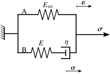
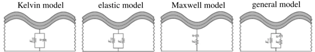
Since we are only interested in the onset of instabilities, unlike the computational approach to this problem, the analytical solution is derived based on small strains instead of finite deformations. In the computational approach, it would be impossible to capture instabilities if geometrical nonlinearities were precluded. Nonetheless, the geometrical instabilities in the analytical approach are implicitly accounted for via a buckling analysis of the film. To study the viscoelastic behavior of the substrate at small strains, we choose a rheological model demonstrated inFigure 4representing the (general) standard solid model to recover a wide range of material behaviors; see[Holzapfel 2000;Simo and Hughes 1998]for further details. As it will be clarified, the (general) standard solid model captures both the Maxwell model and the Kelvin model. The rheological model inFigure 4consists of two spring elements with constants E and E1, which represent the elastic response of the solid. The spring with constant E is connected in series with a dashpot with viscosity ⌘. From a physical point of view, the constants E1, E, and ⌘ must be positive. The strains in both elements A and B are identical due to their parallel arrangement. The total stress prescribed inFigure 4can be recovered as addition of the stress in A and B as
= 1+ ⌫ with 1= E
1", (10)
where 1 is applied to the element B representing the stress of the rheological model as t ! 1 in a
relaxation test and ⌫represents the viscous stress acting on the dashpot. From a mechanical point of
view, the strain in the viscous element B is the addition of the elastic strain in the spring with constant E and the inelastic strain-like internal variable ↵ in the dashpot and thus
E1 E ⌘ " ↵ B A
Figure 4. Illustration of the kinematics of the viscoelastic material with (general) stan-dard solid element model. The rheological model is composed of two elements A and B. The subscript 1 denotes the elastic response of the solid for t ! 1 corresponding to the behavior of solid in a relaxation test after infinite time.
By considering the initial modulus E0 at t = 0 with no strain in the dashpot, the rheological model in Figure 4resembles a solid with two spring elements with constants E and E1 as instantaneous modulus E0= E1+ E and hence,(10)leads to
= E0" E↵, (12)
where the inelastic strain ↵ satisfies the evolution equation ˙↵ +1⌧↵= 1
⌧" with the condition t! 1lim ↵(t) = 0. (13)
Additionally, there exists an alternative formulation by introducing a stress-like variableq = E[" ↵] acting on the dashpot, so that(12)transforms to = E1"+ q and thus the evolution equation(13)can
be rewritten as
˙q +1⌧q = 1⌧E" with the condition lim
t! 1q(t) = 0. (14)
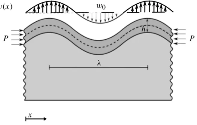
To determine the critical growth of an elastic film on a viscoelastic substrate, we compute the critical growth by analyzing the buckling of the film on the substrate,Figure 5. In doing so, first we assume the substrate to be elastic and then we replace the elastic behavior of the substrate by its equivalent viscoelas-tic one. The whole analysis here is two-dimensional and corresponding to a plane-strain scenario. Let wdenote the deflection of the film. The governing differential equation of a film adhered to an infinite half-space reads 1 12Efh3 d4w dx4 + h d2w dx2 = fs, (15)
where is the stress in the film, Ef is the film elastic modulus and h is the film thickness. The transverse
force on the film from the substrate fsreads[Allen 1969]
fs= 2Es
w(x) w0
P P
x
h
Figure 5. Analytical model of growing elastic film on a viscoelastic substrate. The film thickness is denoted h and is the wavelength. The amplitude of the sinusoidal wave on the substrate is denoted w0. The lateral force P relates to the stress in the film via
P = hb with b being the width of the domain in the direction normal to the plane.
where ⌫sis the Poisson’s ratio of the substrate, with sinusoid w with the wavenumber n on its surface.
By substituting fs in(15)and solving for , we have
=121 Efh2n2+ 2Es
[3 ⌫s][1 + ⌫s]hn, (17)
from which the critical wavenumber can be computed by minimizing with respect to as nc= 3
s
12Es
Ef[3 ⌫s][1 + ⌫s]h3, (18)
from which the critical wavelength can be readily calculated. Inserting the critical wavenumber nc into
the stress equation(17)results in the critical stress c and eventually the critical growth gc is obtained
as gc⇡ "c= c/Ef for sufficiently small values of "c. A more accurate approximation for the critical
growth reads gc= "c/[1 "c]. Nonetheless, the validity of this linear approach is questionable for larger
"ccorresponding to film-to-substrate stiffness ratios less than 10; see[Cao and Hutchinson 2012b].
Now, we generalize the elastic model to a viscoelastic one to study the effect of the viscoelastic material properties of the substrate on the critical growth of the film. To do so, by regarding Esand ⌫s
as the material constants of the substrate, the viscoelastic substrate model can be expressed solely by modifying the material constants of an elastic substrate model. First, by solving the internal variable in
(14)in the linear viscoelastic regime, we have for the elastic modulus of the viscoelastic substrate Es= E1+ E exp
⇣ 1t ⌧
⌘
. (19)
It can be observed that for a large relaxation time ⌧ compared to the growth time 1t, the substrate elastic modulus results in Es= E1+ E, where the substrate can be viewed as an elastic substrate. On the other
hand, for relatively slowly growing film or alternatively small relaxation time, the exponential term tends to 0 resulting in the effective elastic modulus in substrate Es= E1. To formulate this in the governing
Kelvin model elastic model Maxwell model general model
Figure 6. Illustration of four models for the substrate behavior. The standard solid model can recover Maxwell, Kelvin, and elastic models as three special cases.
equations of a growing film on a viscoelastic substrate, we introduce the effective substrate stiffness Eeff s = E1+ [Es E1] exp ⇣ 1t ⌧ ⌘ , (20)
and then by substituting(20)in(16)we obtain the viscoelastic substrate transverse force as
fs= 2 [3 ⌫s][1+⌫s] h E1+ [Es E1] exp ⇣ 1t ⌧ ⌘i nw(x), (21)
and after substituting in(15)and solving for we have =121 Efh2n2+ 2 [3 ⌫s][1+⌫s]hn h E1+ [Es E1] exp⇣ 1t ⌧ ⌘i , (22)
and consequently, the minimization with respect to yields the critical wavenumber nc= 3
s
12[E1+ [Es E1] exp( 1t/⌧)]
Efh3[3 ⌫s][1 + ⌫s] , (23)
from which the critical stress c and eventually the critical growth gc can be calculated, as before.
Obviously, the standard solid model in viscoelastic material modeling can simplify to the Maxwell, Kelvin, and elastic models, as schematically illustrated inFigure 6. For instance, fromFigure 6it is obvious that a standard solid model reduces to the Maxwell model if E1! 0, and thus the effective
stiffness of the substrate in this case reads
Es= E exp ⇣ 1t ⌧ ⌘ , (24) and consequently fs= 2 [3 ⌫s][1+⌫s][Esexp ⇣ 1t ⌧ ⌘ ]nw(x). (25) 4. Numerical examples
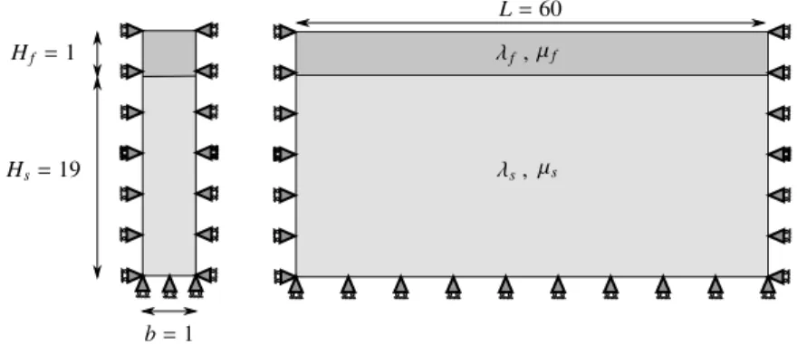
The purpose of this section is to illustrate the growth-induced instabilities in a bilayer system composed of a thin growing film on top of a viscoelastic substrate as shown inFigure 7. In particular, we study the influence of a viscoelastic substrate on the critical wavelength due to growth-induced buckling patterns as well as the critical growth. More importantly, the numerical results obtained from the computational simulations using the finite element method are compared against the proposed analytical solution.
For all examples, to omit further complexities in interpreting the results, it is assumed that the critical growth is reached at the same 1t independent of the stiffness ratio. Therefore, the relaxation time ⌧
f , µf s, µs L = 60 b = 1 Hs=19 Hf =1
Figure 7. Geometry and dimensions of an elastic growing film on a viscoelastic substrate. remains as the only independent parameter to study its effect instead of the ratio 1t/⌧. In order to extend the observations to a more general case with varying 1t, the dimensionless parameter = 1t/⌧ is defined, thereby is essentially the ratio of the time for the film to reach the critical growth over the substrate relaxation time. For the problem of interest here, the neo-Hookean potential
e=12µ[Fe: Fe 2 2 ln Je] +12 ⇥12[Je2 1] ln Je⇤ with Je= det Fe (26)
is used for the elastic response of the film and the substrate where µ and are Lamé parameters. Fur-thermore, it is assumed that the film grows only along its length but not in the vertical direction. The film over substrate stiffness ratio is defined as µf/µs and the Poisson’s ratio for both media is assumed
as ⌫f = ⌫s= 0.45. Thus the larger the stiffness ratio, the more compliant is the substrate compared to
the film. For the numerical simulations, the domain is discretized using biquadratic finite elements to achieve a better accuracy[Javili et al. 2015]. To compute critical growth of the film and folding pattern, the numerical approach based on the large deformation must be calculated. To this aim, first we weigh the strong form of the balance equations(1)with the test function ' 2H10(B0)with the definition ' = 0
on B0'and integrate overB0, yielding the following global weak form:
r'('(x, t)) = Z B0 Grad X ' : P dV Z B0 '· b0dV Z @B0 '· t0dA = 0. (27)
In the frame of finite element analysis, the goal is to solve(27)by vanishing the residual r'('(x, t)). To
obtain this, and find ' such that the residuum vanishes, the Newton–Raphson scheme can be used: r('m+1)= r('m)+ @r
@'· 1', (28)
where index m denotes the iteration number. The derivative of the residual with respect to ' can be described as the stiffness matrix K = @r@': the eigenvalue representation for diagonalizable matrices
[Javili et al. 2015]of a stiffness matrix for a system with n degrees of freedom is Kn⇥n= K1 1⌦ 1+ K2 2⌦ 2+ · · · + Ki i⌦ i+ · · · + Kn n⌦ n=
n
X
i=1
(a) (b) (c)
(d)relaxation
time exp( 1t/t)
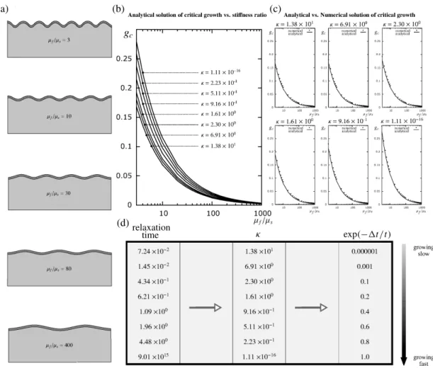
Figure 8. Instability study of growing elastic film with thickness 1 on a viscoelastic substrate by using various relaxation times to examine the viscous substrate effects on the critical growth of the elastic film. The standard solid model is chosen to capture viscoelastic effects. The relation of growth time to relaxation time is = 1t/⌧. The stiffness ratio is µf/µs and the Poisson’s ratio for both the film and substrate is ⌫f =
⌫s = 0.45. The variation of relaxation times occurs by changing the viscosity ⌘ of
the material. This effect could have identical results by holding viscosity constant and changing growth time. The right growing time line shows this parallel impact.
in which Ki represents the eigenvalue and i the associated unit eigenvector for i = 1, . . . , n. In the
sense of studying growth instability, the negative eigenvalue of stiffness matrices represents the growth instability and the associated unit eigenvector represents the folding pattern. To obtain the critical value of growth, the growth is increased until one of the eigenvalues becomes negative. Then, the associated growth is the critical growth of the system. More computational details are explained in theAppendix.
Figure 8gathers the analytical results and numerical simulations using eigenvalue analysis. The critical growth gc inFigure 8, b and c, and corresponding folding pattern inFigure 8a are illustrated for different
c= 17.1 c= 15.0 c= 13.3 = 1.38 ⇥ 101 exp( 1t/t) = 0.000001 = 1.61 ⇥ 100 exp( 1t/t) = 0.2 = 1.11 ⇥ 10 16 exp( 1t/t) = 1.0
Figure 9. Folding of growing film with thickness 1 on a viscoelastic substrate for some = 1t/⌧ with stiffness ratio µf/µs = 40. The Poisson’s ratio for both the film and
substrate is ⌫f = ⌫s= 0.45. The critical wavelength is denoted c= 2⇡/nc, where the
critical wavenumber nc can be calculated from(23).
stiffness ratios µf/µs for various inFigure 8d to study the effect of relaxation time on the critical
growth gc and wavelength. First, we see that for a given ⌧ inFigure 8b, the critical growth decreases by
increasing the stiffness ratio. Second, it is observed that the critical growth gc increases by decreasing
or alternatively increasing the relaxation time ⌧. This can be justified by the first observation. That is, for a given µf/µs, a larger relaxation time ⌧ leads to an increased effective stiffness of the substrate
and hence resembles an overall smaller film-to-substrate stiffness ratio which in turn results in a larger critical growth. Third, there is excellent agreement between the numerical results inFigure 8c using the finite element method via eigenvalue analysis and the proposed analytical solution. So much so that the points corresponding to the numerical results are shown on separate graphs for a better visualization. The numerical results from the finite element method consistently overestimate the analytical solution only and provide an overall stiffer response, as expected. Furthermore, for a given relaxation time, e.g., ⌧ = 0.0724, the deformation is illustrated for various stiffness ratios on the left. Increasing the stiffness ratio results in a larger wavelength and thus less waves for a given length of the domain according to(23). Finally, the folding patterns for a given stiffness ratio of µf/µs= 40 but for varying relaxation time ⌧
are illustrated inFigure 9and it is obvious that increasing the relaxation time decreases the wavelength. This can again be justified by the fact that increasing the relaxation time is effectively decreasing the stiffness ratio and hence the wavelength.
5. Conclusion
Biological growth in living systems can lead to geometric instabilities in the form of folding and wrin-kling, thus understanding these phenomenon is of crucial importance. Growth-induced instabilities are often studied in bilayer systems where both the thin film and the underlying compliant substrate behave elastically. Nonetheless, due to its relevance for living tissues, the substrate in this contribution is con-sidered to be viscoelastic. This problem is carefully analyzed using both an analytical approach as well as computational simulations using the finite element method whereby eigenvalue analysis is utilized to capture the instabilities. The results obtained from both methods are compared for a wide range of parameters and show an excellent agreement between the computational simulations and the proposed analytical solution. It is observed that the viscoelastic influence of the substrate can be interpreted and eventually replaced by an “effective” elastic model. Our next immediate extension of this contribution is to replace the perfect bonding between the substrate and the film by a general interface model[Javili et al. 2017;Javili 2018]and study its implications.
read data: geometrical data, material parameters, and boundary conditions initialization: set degrees of freedom, quadrature points, and shape functions while eigenvalues > 0 do
calculate Neumann, Dirichlet, and loads for this time step while Newton loop do
initialize global tangent stiffness matrix, residuum, volume, surface, and internal forces for element loop do
determine DOFs, displacement, and coordinates belonging to the current element for integration loop do
evaluate shape function and its gradient at the current quadrature point calculate deformation gradient F
if film element then
elasticity material box(F, state variables) else
viscoelasticity material box(F, state variables) end
for node loop do
assemble element stiffness matrix K end
end
assemble global stiffness matrix, volume, surface, and internal forces end calculate residualr'('(X, t)) end eigenvalue analysis if eigenvalue < 0 then g = gcr calculate eigenvector break while loop else
growth increment gnew= gold+ 1g
end end
Algorithm 1. The incremental nonlinear finite element method with eigenvalue analysis to capture geometrical instabilities.
Appendix: Computational aspects
The geometry inFigure 7consists of a rectangular domain which is meshed with 560 quadratic quadrilat-eral elements with 3578 DOFs. Computations are carried out using our in-house nonlinear finite element code; to have a proper numerical solution we use the finite element method algorithm1, which explains the finite element structure using eigenvalue analysis. Algorithm 2is an elastic material box used to model growth of elastic film andAlgorithm 3is a viscoelastic material box to model the substrate behavior.
Input: deformation gradient (F), state variables
Update configurations Jn+1:= det[Fn+1], Cn+1= Fn+1t Fn+1
Decompose F to FeandFg
Calculate growth part Fg
Compute P,C
Output: Piola stress and algorithmic tangent moduli
Algorithm 2. Elastic material box to calculate growth in living materials. Input: deformation gradient (F), state variables
Update configurations Jn+1:= det[Fn+1], Cn+1= Fn+1t Fn+1, Fn+1= Jn+11/3Fn+1,Cn+1= Jn+12/3Cn+1
calculate the second Piola–Kirchhoff stress Sn+1and internal variable Qn+1
Compute P,C
Output: Piola stress, algorithmic tangent moduli
Algorithm 3. Viscoelasticity material box to calculate viscoelastic effects of substrate. References
[Allen 1969] H. G. Allen,Analysis and design of structural sandwich panels, Pergamon, Oxford, 1969.
[Balbi and Ciarletta 2013] V. Balbi and P. Ciarletta,“Morpho-elasticity of intestinal villi”, J. R. Soc. Interface10:82 (2013), art. id. 20130109.
[Ben Amar and Goriely 2005] M. Ben Amar and A. Goriely,“Growth and instability in elastic tissues”, J. Mech. Phys. Solids 53:10 (2005), 2284–2319.
[Budday and Steinmann 2018] S. Budday and P. Steinmann,“On the influence of inhomogeneous stiffness and growth on mechanical instabilities in the developing brain”, Int. J. Solids Struct.132-133 (2018), 31–41.
[Budday et al. 2014] S. Budday, P. Steinmann, and E. Kuhl,“The role of mechanics during brain development”, J. Mech. Phys. Solids72 (2014), 75–92.
[Budday et al. 2015] S. Budday, E. Kuhl, and J. W. Hutchinson,“Period-doubling and period-tripling in growing bilayered systems”, Philos. Mag.95:28-30 (2015), 3208–3224.
[Cao and Hutchinson 2012a] Y. Cao and J. W. Hutchinson, “From wrinkles to creases in elastomers: the instability and imperfection-sensitivity of wrinkling”, Proc. R. Soc. Lond. A468:2137 (2012), 94–115.
[Cao and Hutchinson 2012b] Y. Cao and J. W. Hutchinson,“Wrinkling phenomena in neo-Hookean film/substrate bilayers”, J. Appl. Mech.79:3 (2012), art. id. 031019.
[Ciarletta and Ben Amar 2012] P. Ciarletta and M. Ben Amar,“Growth instabilities and folding in tubular organs: a variational method in non-linear elasticity”, Int. J. Non-Linear Mech.47:2 (2012), 248–257.
[Ciarletta and Maugin 2011] P. Ciarletta and G. A. Maugin,“Elements of a finite strain-gradient thermomechanical theory for material growth and remodeling”, Int. J. Non-Linear Mech.46:10 (2011), 1341–1346.
[Ciarletta et al. 2013] P. Ciarletta, L. Preziosi, and G. A. Maugin,“Mechanobiology of interfacial growth”, J. Mech. Phys. Solids61:3 (2013), 852–872.
[Cowin and Hegedus 1976] S. C. Cowin and D. H. Hegedus,“Bone remodeling, I: Theory of adaptive elasticity”, J. Elasticity 6:3 (1976), 313–326.
[Dervaux and Ben Amar 2011] J. Dervaux and M. Ben Amar,“Buckling condensation in constrained growth”, J. Mech. Phys. Solids59:3 (2011), 538–560.
[Dunlop et al. 2010] J. W. C. Dunlop, F. D. Fischer, E. Gamsjäger, and P. Fratzl,“A theoretical model for tissue growth in confined geometries”, J. Mech. Phys. Solids58:8 (2010), 1073–1087.
[Epstein and Maugin 2000] M. Epstein and G. A. Maugin,“Thermomechanics of volumetric growth in uniform bodies”, Int. J. Plast.16:7-8 (2000), 951–978.
[Garikipati et al. 2004] K. Garikipati, E. M. Arruda, K. Grosh, H. Narayanan, and S. Calve,“A continuum treatment of growth in biological tissue: the coupling of mass transport and mechanics”, J. Mech. Phys. Solids52:7 (2004), 1595–1625.
[Goriely et al. 2008] A. Goriely, M. Robertson-Tessi, M. Tabor, and R. Vandiver,“Elastic growth models”, pp. 1–44 in Mathe-matical modelling of biosystems, edited by R. P. Mondaini and P. M. Pardalos, Appl. Optim.102, Springer, 2008.
[Holzapfel 2000] G. A. Holzapfel, Nonlinear solid mechanics: a continuum approach for engineering, Wiley, Chichester, England, 2000.
[Hong et al. 2009] W. Hong, X. Zhao, and Z. Suo,“Formation of creases on the surfaces of elastomers and gels”, Appl. Phys. Lett.95:11 (2009), art. id. 111901.
[Huang 2005] R. Huang,“Kinetic wrinkling of an elastic film on a viscoelastic substrate”, J. Mech. Phys. Solids53:1 (2005), 63–89.
[Huang and Suo 2002] R. Huang and Z. Suo,“Instability of a compressed elastic film on a viscous layer”, Int. J. Solids Struct. 39:7 (2002), 1791–1802.
[Huang et al. 2005] Z. Y. Huang, W. Hong, and Z. Suo,“Nonlinear analyses of wrinkles in a film bonded to a compliant substrate”, J. Mech. Phys. Solids53:9 (2005), 2101–2118.
[Hutchinson 2013] J. W. Hutchinson,“The role of nonlinear substrate elasticity in the wrinkling of thin films”, Phil. Trans. R. Soc. A371:1993 (2013), art. id. 20120422.
[Javili 2018] A. Javili,“Variational formulation of generalized interfaces for finite deformation elasticity”, Math. Mech. Solids 23:9 (2018), 1303–1322.
[Javili et al. 2013] A. Javili, A. McBride, and P. Steinmann,“Thermomechanics of solids with lower-dimensional energetics: on the importance of surface, interface, and curve structures at the nanoscale”, Appl. Mech. Rev.65:1 (2013), art. id. 010802. [Javili et al. 2014] A. Javili, P. Steinmann, and E. Kuhl,“A novel strategy to identify the critical conditions for growth-induced
instabilities”, J. Mech. Behav. Biomed. Mater.29 (2014), 20–32.
[Javili et al. 2015] A. Javili, B. Dortdivanlioglu, E. Kuhl, and C. Linder,“Computational aspects of growth-induced instabilities through eigenvalue analysis”, Comput. Mech.56:3 (2015), 405–420.
[Javili et al. 2017] A. Javili, P. Steinmann, and J. Mosler,“Micro-to-macro transition accounting for general imperfect inter-faces”, Comput. Methods Appl. Mech. Eng.317 (2017), 274–317.
[Jin et al. 2011] L. Jin, S. Cai, and Z. Suo,“Creases in soft tissues generated by growth”, Europhys. Lett.95:6 (2011), art. id. 64002.
[Jin et al. 2015] L. Jin, A. Auguste, R. C. Hayward, and Z. Suo,“Bifurcation diagrams for the formation of wrinkles or creases in soft bilayers”, J. Appl. Mech.82:6 (2015), art. id. 061008.
[Kuhl 2014] E. Kuhl,“Growing matter: a review of growth in living systems”, J. Mech. Behav. Biomed. Mater.29 (2014), 529–543.
[Kuhl and Steinmann 2003] E. Kuhl and P. Steinmann,“Mass- and volume-specific views on thermodynamics for open sys-tems”, Proc. R. Soc. Lond. A459:2038 (2003), 2547–2568.
[Kuhl et al. 2003] E. Kuhl, A. Menzel, and P. Steinmann,“Computational modeling of growth”, Comput. Mech.32:1-2 (2003), 71–88.
[Li et al. 2011] B. Li, Y.-P. Cao, X.-Q. Feng, and H. Gao,“Surface wrinkling of mucosa induced by volumetric growth: theory, simulation and experiment”, J. Mech. Phys. Solids59:4 (2011), 758–774.
[Moulton and Goriely 2011] D. E. Moulton and A. Goriely,“Circumferential buckling instability of a growing cylindrical tube”, J. Mech. Phys. Solids59:3 (2011), 525–537.
[Podio-Guidugli 2000] P. Podio-Guidugli,“A primer in elasticity”, J. Elasticity58:1 (2000), 1–104.
[Rodriguez et al. 1994] E. K. Rodriguez, A. Hoger, and A. D. McCulloch,“Stress-dependent finite growth in soft elastic tissues”, J. Biomech.27:4 (1994), 455–467.
[Simo and Hughes 1998] J. C. Simo and T. J. R. Hughes,Computational inelasticity, Interdisc. Applied Math.7, Springer, 1998.
[Sultan and Boudaoud 2008] E. Sultan and A. Boudaoud,“The buckling of a swollen thin gel layer bound to a compliant substrate”, J. Appl. Mech.75:5 (2008), art. id. 051002.
[Sun et al. 2012] J.-Y. Sun, S. Xia, M.-W. Moon, K. H. Oh, and K.-S. Kim,“Folding wrinkles of a thin stiff layer on a soft substrate”, Proc. R. Soc. Lond. A468:2140 (2012), 932–953.
[Taber 1995] L. A. Taber,“Biomechanics of growth, remodeling, and morphogenesis”, Appl. Mech. Rev.48:8 (1995), 487–545. [Tepole et al. 2011] A. B. Tepole, C. J. Ploch, J. Wong, A. K. Gosain, and E. Kuhl,“Growing skin: a computational model for
skin expansion in reconstructive surgery”, J. Mech. Phys. Solids59:10 (2011), 2177–2190.
[Wiggs et al. 1997] B. R. Wiggs, C. A. Hrousis, J. M. Drazen, and R. D. Kamm,“On the mechanism of mucosal folding in normal and asthmatic airways”, J. Appl. Physiol.83:6 (1997), 1814–1821.
[Wyczalkowski et al. 2012] M. A. Wyczalkowski, Z. Chen, B. A. Filas, V. D. Varner, and L. A. Taber,“Computational models for mechanics of morphogenesis”, Birth Defects Res. C Embryo Today96:2 (2012), 132–152.
[Xie et al. 2014] W.-H. Xie, B. Li, Y.-P. Cao, and X.-Q. Feng,“Effects of internal pressure and surface tension on the growth-induced wrinkling of mucosae”, J. Mech. Behav. Biomed. Mater.29 (2014), 594–601.
[Xu et al. 2010] G. Xu, A. K. Knutsen, K. Dikranian, C. D. Kroenke, P. V. Bayly, and L. A. Taber,“Axons pull on the brain, but tension does not drive cortical folding”, J. Biomech. Eng. (ASME)132:7 (2010), art. id. 071013.
[Xu et al. 2014] F. Xu, M. Potier-Ferry, S. Belouettar, and Y. Cong,“3D finite element modeling for instabilities in thin films on soft substrates”, Int. J. Solids Struct.51:21-22 (2014), 3619–3632.
[Yavari 2010] A. Yavari,“A geometric theory of growth mechanics”, J. Nonlinear Sci.20:6 (2010), 781–830. Received 3 Aug 2018. Revised 2 Sep 2018. Accepted 9 Sep 2018.
IMANVALIZADEH: [email protected]
Department of Mechanical Engineering, TU-Dortmund, Dortmund, Germany
PAULSTEINMANN: [email protected]
Chair of Applied Mechanics, Universität Erlangen-Nürnberg, Erlangen, Germany and
Glasgow Computational Engineering Centre, School of Engineering, University of Glasgow, Glasgow, UK
ALIJAVILI: [email protected]
Department of Mechanical Engineering, Bilkent University, Ankara, Turkey