Gibbs random field model based 3-D motion estimation from video sequences
Tam metin
Şekil
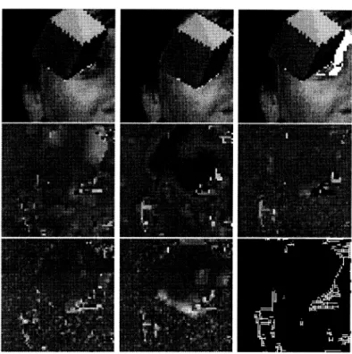
![Figure 5. Estimated w, w aild W2 parameter values of the motion. [up row: left to right]](https://thumb-eu.123doks.com/thumbv2/9libnet/5766635.116819/11.928.252.645.122.386/figure-estimated-aild-parameter-values-motion-left-right.webp)
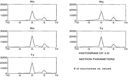
![Figure 9. Estimated w, w and w parameter values of the motion. [up row: left to right]](https://thumb-eu.123doks.com/thumbv2/9libnet/5766635.116819/13.927.254.646.129.389/figure-estimated-parameter-values-motion-row-left-right.webp)
Benzer Belgeler
Our results provide closed from expressions describing the change of the energy-optimum operating point of CSMA networks as a function of the number of nodes (for single-hop
Another low-complexity UWB range estimation algorithm is ‘serial backward search’ (SBS), which estimates the range by searching energy samples in the back- ward direction (i.e., in
Finally this study has assisted us to understand how women blurred the boundaries between public and private realms in the case of the Saturday Mothers and to
Figure 5b shows the average NRET rate for a CdTe D −A pair as a function of the distance, when the donor is an NW and the acceptor is a QW.. In this computation, we made
“Destan” türünün tek tip bir edebiyat alanını imlemiyor olması, gezgin- ci destancılığın sözlü, yazılı/matbu ve elektronik sözlü kültür ortamları içindeki
While we find no obvious candidates in human low and mid-level visual cortex for an explicit representation of specular reflectance from motion, we do find several areas with
We studied human-in-the-loop physical systems with uncertainties due to failures and/or modeling inac- curacies, a set-theoretic model reference adaptive control law at the inner
However, before the I(m)Press, my other project ideas were not actually corresponding to typography. Therefore, I received a suggestion to make an artist’s book with an efficient
