Generalized filtering configurations with applications in digital and optical signal and image processing

i й fe ? ê fe à T ^ *1 ч "*■

_{r III'® i »"blö I«.}

í fi î u i T â ! Ä ^ li ii 'ş i i i i к I“' ^ îÎ ■

_{B ^ t í b ñ i .}

_Λκΰ

_{' ϋί η υ ^ 4 · ^}

i-1'·

_л...

I f O i f

• K 8 &

GENERALIZED FILTERING CONFIGURATIONS WITH

APPLICATIONS IN DIGITAL AND OPTICAL SIGNAL AND

IMAGE PROCESSING

A DISSERTATION

SUBMITTED TO THE DEPARTMENT OF ELECTRICAL AND ELECTRONICS ENGINEERING

AND THE INSTITUTE OF ENGINEERING AND SCIENCES OF BILKENT UNIVERSITY

IN PARTIAL FULFILLMENT OF THE REQUIREMENTS FOR THE DEGREE OF

DOCTOR OF PHILOSOPHY

By

Mehmet Alper Kutay

ЫН

4 0 4 ■ness І93Э

I certify that I have read this thesis and that in my opinion it is fully adequate, in scope and in quality, as a thesis for the degree o f Doctor o f Philosophy.

Haldun M. Özaktaş, PKD. (Supervisor)

I certify that I have read this thesis and that in my opinion it is fully adequate, in scope and in quality, as a thesis for the degree o f Doctor of Philosophy.

Enis Çetin, Ph.D.

I certify that I have read this thesis and that in my opinion it is fully adequate, in scope and in quality, as a thesis for the degree o f Doctor o f Philosophy.

I certify that I have read this thesis and that in my opinion it is fully adequate, in scope and in quality, as a thesis for the degree o f Doctor o f Philosophy.

Mefharet Kocatepe, Ph.D.

I certify that I have read this thesis and that in my opinion it is fully adequate, in scope and in quality, as a thesis for the degree o f Doctor o f Philosophy.

^ ' ^ - 0 h r \

Gozde Bozda^, Ph.D.

Approved for the Institute of Engineering and Sciences:

lehmet Baray,

ABSTRACT

GENERALIZED FILTERING CONFIGURATIONS W iTH

APPLICATIONS IN DIGITAL AND OPTICAL SIGNAL AND

IMAGE PROCESSING

Mehmet Alper Kutay

Ph. D. in Electrical and Electronics Engineering Supervisor: Dr. Haldun M . Ozakta§

February 24, 1999

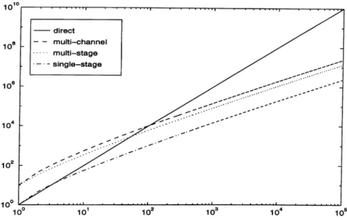
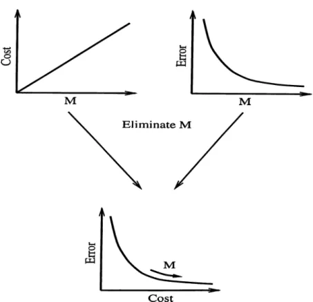
In this thesis, we first give a brief summary o f the fractional Fourier transform which is the generalization o f the ordinary Fourier transform, discuss its importance in optical and digital signal processing and its relation to time-frequency representations. We then introduce the concept o f filtering circuits in fractional Fourier domains. This concept unifies the multi-stage (repeated) and multi-channel (parallel) filtering configurations which are in turn generalizations o f single domain filtering in fractional Fourier domains. We show that these filtering configurations allow a cost-accuracy trade­ off by adjusting the number of stages or channels. We then consider the application of these configurations to three important problems, namely system synthesis, signal synthesis, and signal recovery, in optical and digital signal processing. In the system and signal synthesis problems, we try to synthesize a desired system characterized by its kernel, or a desired signal characterized by its second order statistics by using fractional Fourier domain filtering circuits. In the signal recovery problem, we try to recover or estimate a desired signal from its degraded version. In all of the examples we give, significant improvements in performance are obtained with respect to single domain filtering methods with only modest increases in optical or digital implementation costs. Similarly, when the proposed method is compared with the direct implementation of general linear systems, we see that significant computational savings are obtained with acceptable decreases in performance.

Keywords:

Fractional Fourier transforms, optical signal processing, signal and system synthesis, signal recovery, time- or space-varying filtering

ÖZET

G E N E L L E N M İŞ S Ü Z G E Ç L E M E K O N F İG U R A S Y O N L A R I V E B U N L A R IN S A Y IS A L V E O P T İK S E L İŞ A R E T V E G Ö R Ü N T Ü

İŞL E M E D E K İ U Y G U L A M A L A R I

Mehmet Alper Kutay

Elektrik ve Elektronik Mühendisliği Doktora Tez Yöneticisi: Dr. Haldun M . Özaktaş

24 Şubat 1999

Bu tezde ilk olarak bilinen Fourier dönüşümünün bir genellemesi olan kesirli Fourier dönüşümünün kısa bir özeti verildi ve bu dönüşümün optiksel ve sayısal işaret işlemedeki önemi ve zaman-frekans gösterimleri ile olan bağlantısı üzerinde duruldu. Daha sonra kesirli Fourier dümenlerinde süzgeçleme devreleri kavramı ortaya konuldu. Bu kavram tek aşamalı süzgeçleme yönteminin genellemesi olan çokaşamalı ve cokkanallı süzgeçleme konfigürasyonlarmı bir çatı altında birleştirmekte ve herhangi bir uygulamada doğruluk maliyet değiş-tokuşu yapma olanağı sağlamaktadır. Bu süzgeçleme devre konfigürasy- onlarmm optiksel ve sayısal işaret işlemedeki çok önemli üç problem olan sistem sentezi, işaret sentezi ve işaret iyileştirmedeki uygulamaları üzerinde duruldu. Sistem ve işaret sentezi uygulamalarında çekirdek fonksiyonu ile tanımlanan istenen bir sistem, veya ikinci-derece istatistiksel özellikleri ile tasvir edilen istenen bir işaret kesirli Fourier domeni süzgeçleme devresi kullanılarak sentezlenmeye çalışılmıştır, işaret elde edimi veya iyileştirilmesi uygulamasında ise bozulmuş istenen bir işaret iyileştirilmeye veya kestirilmeye çalışılmıştır. Bütün bu örneklerde, süzgeçleme devresi metodumuz tek bir bölgecikte uygulanan filtreleme metodları ile karşılaştırıldığında, optik veya nümerik uygulama konusundaki masrafları fazla artırmadan sistem performansının cok daha fazla geliştirilebileceği gösterilmiştir. Benzer olarak, önerdiğimiz metod genel doğrusal sistemler ile karşılaştırıldığında, yeterli olabilecek sistem performanslarının çok daha düşük masraf karşılığı bizim metodumuzla elde edilebileceği anlaşılmıştır.

Anahtar Kelimeler: Kesirli Fourier dönüşümü, optiksel işaret işleme, işaret ve sistem

sentezi, işaret iyileştirilmesi, zaman veya mekan ile değişen süzgeçleme

AC K N O W LED G M EN TS

Many people have contributed to the development o f this thesis. But above all, I would like to express my deepest gratitude to Dr. Haldun M. Ozaktaş for his supervision, constructive suggestions, and encouragement throughout the development o f this work. It is also my pleasure to thank our research group members Dr. Fatih Erden, Ayşegül Şahin, Çağatay Candan and Özgür Güleryüz for their valuable input and many useful discussions.

Special thanks should go to Dr. Orhan Arikan for many useful suggestions and discussions throughout Ph.D. study.

I would like to thank Dr. Enis Çetin, Dr. Mefharet Kocatepe, and Dr. Gözde Bozdağı for reading the manuscript and commenting on the thesis.

The graduate students at the EE department provided me great support. I would also like to thank all o f my friends for their suggestions and encouragement.

Finally, I want to express my sincere thanks to my dearest Bahar for her love, generosity and patience, and also to our families for their encouragement, help, and support.

Contents

1 Introduction 1

2 The Fractional Fourier Transform 5

2.1 Introduction and H isto ry ... 5

2.2 Definition and P roperties... 7

2.2.1 Eigenvalues and Spectral Expansion... 10

2.2.2 Operational p r o p e r tie s ... 12

2.2.3 Relation to the Wigner d istribu tion ... 12

2.2.4 Fractional Fourier D o m a i n s ... 15

2.3 Optical And Digital Implementation ... 16

2.4 Discrete Fractional Fourier Transform ... 18

2.5 Generalization to Two-Dimensional S y s t e m s ... 19

2.5.1 Separable Two-Dimensional Fractional Fourier Transformation . . 19

2.5.2 Non-separable Two-Dimensional Fractional Fourier Transformation 20 3 Generalized Filtering Configurations Based on Fractional Fourier Transforms 22 3.1 Single-stage Filtering in Fractional Fourier D om a in s... 23

3.2 Multi-Stage Filtering in Fractional Fourier D o m a in s... 27

3.3 Multi-Channel Filtering in Fractional Fourier D o m a in s ... 29

3.4 Filtering C ir c u i t s ... 31

3.5 Discrete F orm u la tion ... 32

3.5.1 Extension to the Rectangular C a s e ... 34

3.5.2 Complexity A n a ly s is ... 35

3.6 D iscu ssion ... 38

4 Applications in System Synthesis 43 4.1 General Linear System Synthesis ... 46

4.1.1 Solution o f the System Synthesis P r o b l e m ... 50

4.1.2 E xtensions... 53

4.2 Examples ... 54

5 Applications in Signal Synthesis 58 5.1 Signal Synthesis... 58

5.2 E x a m p le s ... 66

6 Applications in Signal Recovery 73 6.1 Signal Recovery and Restoration... 73

6.2 E x a m p le s ... 82

7 Conclusions and Future W ork 89

List of Figures

1.1 Filtering configurations... 2

2.1 Oblique integral projections o f the Wigner distribution... 15

3.1 Filtering in a transform d o m a in ... 24

3.2 Filtering in a fractional Fourier d o m a in ... 26

3.3 Filtering in multiple fractional Fourier d o m a i n s ... 28

3.4 Multi-stage filtering in fractional Fourier d o m a in s ... 28

3.5 Multi-channel filtering in fractional Fourier d om a in s... 30

3.6 Fractional Fourier domain filtering circuit... 31

3.7 Cost comparison o f exact and approximate implementations o f linear systems... 37

3.8 Cost-accuracy trade-off. ... 39

3.9 Short-time fractional Fourier filte r ... 42

4.1 Reverse perfect shuffle interconnection architecture. (After [ 1 3 ] ) ... 56

5.1 Mutual intensity synthesis p r o b le m ... 60

5.2 The expansion coefficients in GSM beam and corresponding mutual intensity fu n c tio n ... 68

5.4 Normalized error versus number o f filte r s ... 70

5.5 The expansion coefficients o f the desired GSM beam and corresponding mutual intensity fu n ction ... 71

5.6 The expansion coefficients o f the given and desired GSM b e a m s ... 71

5.7 The mutual intensity functions o f the desired and synthesized GSM beams 72 6.1 Observation model for the degraded s i g n a l ... 74

6.2 Pre-compensation filter configuration... 75

6.3 Post-compensation filter configuration... 75

6.4 Image restoration with pre-compensation filter co n fig u ra tio n ... 83

6.5 Image restoration with post-compensation filter configuration... 84

6.6 Normalized error versus number o f filte r s ... 85

6.7 The filtering circuit used in image r e s t o r a t io n ... 85

6.8 Restoration o f a signal corrupted by additive chirp n o i s e ... 86

6.9 Denoising e x a m p l e ... 87

6.10 Wigner distribution o f a signal with quadratic instantaneous frequency . 88 6.11 Denoising o f a signal with quadratic instantaneous freq u en cy ... 88

Chapter 1

Introduction

In many applications in signal processing and optical information processing, it is desired to implement linear systems. Linear systems are easy to handle and can describe many phenomenon in real life to a good approximation. A general linear system is characterized by the relation,

g{u)

= j

H{u,u')f{u')du\

(1.1) where

H{u,u')

is called the kernel o f the system. Equation 1.1 can be discretized as

N - l

9k

Hknfn·

n=0

(

1

.

2

)

The last equation, which is simply a matrix-vector multiplication, may either represent a system which is inherently discrete or may constitute an approximation o f its continuous version. Digital implementation o f such general linear systems takes

O(N^)

time. Common single-stage optical implementations, such as optical matrix-vector multiplier architectures or multi-facet architectures [1, 2] require an optical system whose space- bandwidth product is

O(N^).

A widely known sub-class o f general linear systems is linear shift-invariant or convolution type systems which are characterized by kernels o f the special form

H{u,u')

=

h{u — u')

or

Hkn

=

hk-n·

Ordinary Fourier transformation is a very important operator in the analysis of such systems because these systems correspond to multiplication with a filter function in the Fourier domain. Their digital implementation takes

0{N \ogN )

time (by using the FFT algorithm) and their optical implementation

requires an optical system whose space-bandwidth product is

0 (N ).

This efficiency in the implementation o f such systems leads them to play an important role in digital signal processing and optical information processing. In most o f the signal restoration (deblurring, denoising), reconstruction and enhancement problems the operators involved are approximated by shift-invariant systems [3, 4, 5]. These approximations are sometimes justified and the use of convolution type systems is fully adequate. However in other cases, their use is either totally inappropriate or at best a crude approximation which is employed only because o f their significantly lower digital or optical implementation cost. This is not surprising given the fact that shift-invariant systems are a much more restrictive class than general linear systems, which is evident upon noting that general linear systems have degrees o f freedom whereas shift- invariant systems have only

N.

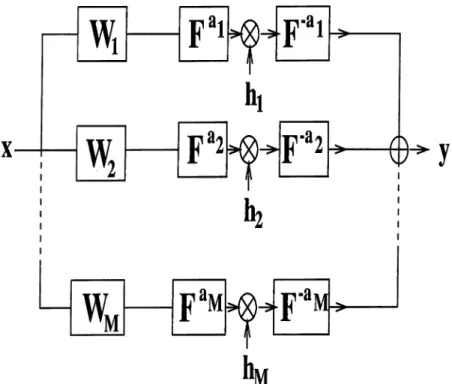
(a)

h

1 - 1

g

f

(b)

h

1-a

g

(C) F F ^ h . F ' “ M i-^ g *M

id)

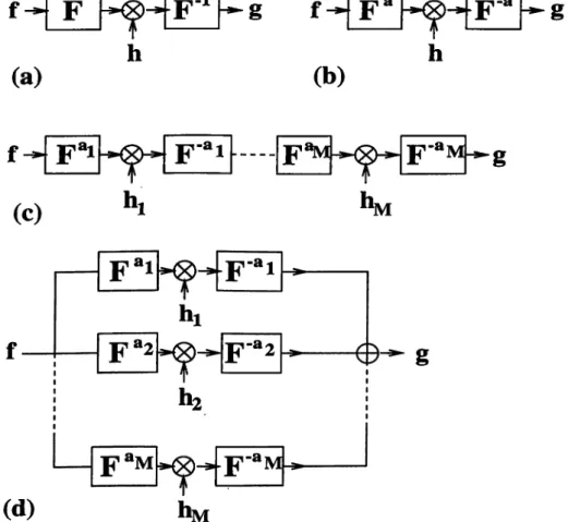
_{‘ M}

Figure 1.1: Single-stage filtering in the Fourier domain (a), and the ath order fractional Fourier domain (b). Repeated (multi-stage or series) filtering in fractional Fourier domains (c). Multi-channel (parallel) filtering in fractional Fourier domains (d).

We may think o f shift-invariant systems and general linear systems as representing two extremes in a cost-accuracy tradeoff: the general systems have O(iV^) degrees of freedom and can be implemented with O(iV^) cost and, shift-invariant systems have

0 {N )

degrees o f freedom and can be implemented with

0 {N log N)

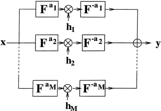
cost. Sometimes use o f shift-invariant systems may be inadequate, but at the same time use o f general linear systems may be overkill and prohibitively costly. In such situations where both extremes are unacceptable, or simply when we desire greater flexibility in trading off between cost and accuracy, it would be desirable to be able to interpolate between these two extremes. There may be many ways of achieving this. One such way is the use o f filtering in fractional Fourier domains [6]. Common single-stage Fourier-domain filtering is shown in Fig. 1.1 (a). Fig. 1.1 (b) depicts single-stage filtering in the ath order fractional Fourier domain. In this configuration the Fourier transform blocks in Fig. 1.1 (a) are simply replaced by the fractional Fourier transform blocks. It has been shown that in some cases this configuration enables significant improvements. More detailed discussion with applications are given in [7, 8, 9, 10, 11, 12]. A generalization o f the single-stage fractional Fourier domain filtering is the repeated or multi-stage filtering in fractional Fourier domains and this configuration is shown in Fig. 1.1 (c). In this configuration

M

single stage fractional Fourier domain filters (Fig. 1.1 (b)) are combined in series so that the output o f this configuration is obtained by applying

M

single fractional Fourier domain filters consecutively to the input. The input is first transformed into the aith domain where it is multiplied by a filter

hi(u).

The result is then transformed back into the original domain. This process is repeated

M

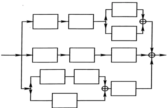
times. This configuration was first proposed in [6] and explored in detail in [13, 14, 15, 16]. A dual configuration is the multi-channel filtering in fractional Fourier domains which is shown in Fig. 1.1 (d). This configuration was first suggested by Orhan Arikan. In this thesis, the multi-channel filtering configuration will be discussed in detail and a further generalization, filtering circuits in fractional Fourier domains will be introduced. Applications o f these filtering circuits in digital signal and optical information processing will be given.

The fractional Fourier transform is the generalization o f the ordinary Fourier transform. Given this, every property and application o f the common Fourier transform becomes a special case o f that o f the fractional transform. A comprehensive discussion with some properties and its relation to well-known physical, optical and signal processing concepts are summarized in a chapter [17] and in more detail in a forthcoming book [18].

We here summarize what is eichieved in this thesis. One of the most important property of the fractional Fourier transform is its relation to the Wigner distribution and ambiguity function. We have shown that this property generalizes to certain other time-frequency distributions belonging to the so-called Cohen class [19].

In order to successfully apply the transform to digital signal processing applications, we need to calculate the transform digitally. We have developed an efficient algorithm

{0 {N

log

N))

for the computation o f the fractional Fourier transform [20]. This algorithm also leads to a definition for the discrete fractional Fourier transform. However, this definition does not satisfy exactly some o f the essential properties o f the discrete transform. Thus we have proposed a discrete fractional definition by finding the oth power of the discrete Fourier transform (DFT) matrix and showed that this definition is fully analogous to the continuous definition [21, 22, 23].

As a main application o f the transform in signal processing, we have first introduced the concept of filtering in a single fractional Fourier domain [7, 8, 10]. We then applied the algorithm to image restoration problems and discussed some o f the issues that do not exist for one-dimensional signals [12]. We improved the performance o f the image restoration algorithm by using the non-separable definition of the transform [24].

The idea o f single-domain filtering has been further generalized to multi-stage (repeated) filtering in fractional domains [13, 14, 15]. Recently we have proposed a dual configuration which is the multi-channel filtering [25, 26, 27, 28]. In this thesis we unify all these filtering configurations and discuss their applications under three main headings: system synthesis, signal synthesis and signal recovery.

The outline of the thesis is as follows. In chapter 2, we introduce the fractional Fourier transformation. We define it mathematically, discuss some o f its properties including its relationship with the Wigner distribution and quadratic-phase systems, and generalize its definition to two-dimensions. We will also discuss the discrete fractional Fourier transformation. Then in chapter 3, we introduce the concept o f filtering circuits in fractional Fourier domains. We first overview the single and multi-stage (repeated) fractional Fourier domain filtering configurations and then discuss in detail multi-channel (parallel) filtering configuration and unify all these configurations under the concept of filtering circuits in fractional Fourier domains. In chapters 4 , 5 and 6 we will give applications o f filtering circuits in fractional Fourier domains with some simulation examples. Finally, conclusions and future work in this field are discussed in Chapter 7.

Chapter 2

The Fractional Fourier Transform

The filtering circuits concept introduced in this thesis depends mainly on the fractional Fourier transformation. In this chapter we introduce this transform and discuss some of its properties that motivate the applications in signal processing. We will also discuss the discrete fractional Fourier transform. Most o f the material in this chapter is adopted from [17].

2.1

Introduction and History

The fractional Fourier transform is a generalization o f the ordinary Fourier transform with an order parameter

a.

Mathematically, the ath order fractional Fourier transform is the ath power o f the Fourier transform operator. The

a

= 1st order fractional transform is the ordinary Fourier transform. The ordinary frequency domain is merely a special case of a continuum o f fractional Fourier domains that will be introduced later. Every property and application o f the common Fourier transform becomes a special case of that o f the fractional transform. In every area in which Fourier transforms and frequency domain concepts are used, there exists the potential for generalization and improvement by using the fractional transform. For instance, the theory of optimal Wiener filtering in the ordinary Fourier domain can be generalized to optimal filtering in fractional domains, resulting in smaller mean-square errors at practically no additional cost [8, 11, 12].

f{u )

and its Fourier transform F (//). The 0th order transform is simply the function itself, whereas the 1st order transform is its Fourier transform. The 0.5th transform is something in between, such that the same operation that takes us from the original function to its 0.5th transform will take us from its 0.5th transform to its ordinary Fourier transform. More generally, index additivity is satisfied; The a

2

th transform of the oith transform is equal to the (a

2

+

ai)th transform. The —1th transform is the inverse Fourier transform, and the —oth transform is the inverse o f the ath transform.

Early papers related to the fractional Fourier transform include [29, 30, 31, 32]. O f importance are two separate streams of mathematical papers which appeared throughout the eighties [33, 34, 35, 36]. However, the number o f publications exploded only after the introduction o f the transform to the optics and signal processing communities [37, 38, 39, 40, 42]. Not all o f these authors were aware o f each other or building on the work of those preceding them, nor is the transform always immediately recognizable in some o f these works.

The fractional Fourier transform (or essentially equivalent transforms) appear in many contexts, although it has not always been recognized as being the fractional power of the Fourier transform and thus referred to as the fractional Fourier transform. For instance, the Green’s function of the quantum-mechanical harmonic oscillator is the kernel o f the fractional Fourier transform. Also, the fractional Fourier transform is a special case o f the more general linear canonical transform [43]. This transform has been studied in many contexts, but again the particular special case which is the fractional Fourier transform has usually not been recognized as such.

The above does not represent a complete list o f known historical references. For a more complete list and also a more comprehensive treatment o f the fractional Fourier transform and its relation to phase-space distributions, we refer the reader to [17] and a forthcoming book [18].

Given the widespread use o f the ordinary Fourier transform in science and engineering, it is important to recognize this integral transform as the generalization of the Fourier transform. Indeed, it has been this recognition which has inspired most of the many recent applications. Replacing the ordinary Fourier transform with the fractional Fourier transform (which is more general and includes the ordinary Fourier transform as its special case) adds an additional degree o f freedom to the problem, represented by the order parameter

a.

This in turn may allow either a more general formulation o f the problem (as in the optical propagation) or improvements based on

the possibility o f optimizing over a (as in the optimal Wiener filtering example).

The fractional Fourier transform has been found to have several applications in the area known as

analog optical information processing,

or

Fourier optics.

This transform allows a reformulation o f this area in a way much more general than that found in standard texts on the subject. It has also led to generalizations of the notions o f space (or time) and frequency domains, which are central concepts in

signal processing,

leading to many applications in this area.

More specifically, some applications which have already been investigated or suggested include diffraction theory [41, 44, 45, 46, 47], optical beam propagation and spherical mirror resonators (lasers) [48, 49], propagation in graded index media [37, 38, 39, 50, 51, 52], Fourier optics [45, 53, 54, 55, 56], statistical optics [57, 58], optical systems design [59, 60], quantum optics[61, 62], radar, phase retrieval [63], tomography [64, 65, 66], signal detection, correlation and pattern recognition [51, 67, 68, 69, 70], space- or time-variant filtering [6, 8, 11, 12, 13, 15, 25, 71, 72, 73, 74], signal recovery, restoration and enhancement [8, 14, 15, 16, 26, 27, 28, 75], multiplexing and data compression [6], study o f space- or time-frequency distributions [19, 42, 65, 76], and solution of differential equations [33, 34]. These are only a fraction of the possible applications.

2.2

Definition and Properties

The ath order fractional Fourier transform of the function

f{u )

will most often be denoted by

fa{u)

or equivalently

F^f{u).

The transform is defined as a linear integral transform with kernel

Ka(u,u')\

fa(u)

=

= f K,(u,u')f(u')du'.

(

2

.

1

)

The kernel will be given explicitly below. All integrals are from minus to plus infinity unless otherwise stated. We prefer to use the same dummy variable

u

both for the original function in the space (or time) domain, and its fractional Fourier transform. This is in contrast to the conventional practice associated with the ordinary Fourier transform, where a different symbol, say

p,,

denotes the argument o f the Fourier transform

F{p)·.

/ ( « ) = I

(2.3)

When it is desirable to distinguish the argument o f the transformed function from that of the original function, we will let

Ua

denote the argument o f the ath order fractional Fourier transform: /«(wo) = (•^“ [/(^)])(w o)· With this convention, uq corresponds to

u,

the space (or time) coordinate,

ui

corresponds to the spatial (or temporal) frequency coordinate

fx,

and

U

2

=

—

uq

, U

3

=

—Ui.

We will refer to or simply as the oth order fractional Fourier transform operator. This operator transforms a function

f{u )

into its fractional Fourier transform

fa{u)·

/ is a finite energy signal and

f{u )

is a finite energy function which are well behaved in the sense usually presumed in physical applications.

After introducing the notation, we now define the ath order fractional Fourier transform

fa{u)

through the following linear integral transform:

fa{u) =

j

Ka{u,u')f{u')du\

Ka{u, u')

=

Atj,

exp [¿7r(cot

— 2

CSC (f>

uv!

+ cot

(j)

u '^ )],

(2.4) where UTT =

\/\ — i

cot

(f

) . (2.5)

(

2

.

6

)

The square root is defined such that the argument o f the result lies in the interval ( —

7

t/

2

,

7

t/

2

]. The kernel is not strictly defined when

a

is an even integer. However, it is possible to show that as

a

approaches an even integer, the kernel behaves like a delta function under the integral sign. Thus, consistent with the limiting behavior o f the above kernel for values o f

a

approaching even integers, we define

K^j{u, u') = S{u — u')

and

K^j±

2

{u,u')

= J(u + u'), where

j

is an arbitrary integer. Generally speaking, the fractional Fourier transform o f

f{u )

exists under the same conditions under which its Fourier transform exists [34, 42].

We first examine the case when

a

is equal to an integer

j.

We note that by definition and correspond to the identity operator

I

and the parity operator

V

respectively (that is,

f

4

j{u)

=

f{u )

and

f

4

j±

2

{u)

= / ( - « ) ) · For a = 1 we find

<j> =

7t/2 ,

A^

= 1, and

We see that

fi{u)

is equal to the ordinary Fourier transform o f

f{u ),

which was previously denoted by the conventional upper case

F{u).

Likewise, it is possible to see that

f-i{u )

is the ordinary inverse Fourier transform o f

f(u ).

Our definition o f the fractional Fourier transform is consistent with defining integer powers o f the Fourier transform through repeated application (that is, =

T F ,

and so on). Since

cj)

= aTr/2 appears in equation 2.4 only in the argument o f trigonometric functions, the definition is periodic in

a

(or

<f))

with period 4 (or 27t). Thus it is sufficient to limit attention to the interval

a

G [—2,2). These facts can be restated in operator notation:

= X ,

where

j, f

are arbitrary integers.

Let us now examine the behavior o f the kernel for small |a| > 0:

g-i7rsgn(</>)/4

Ka(u,

u')

= — — exp[i7r(u -

u ' f /(!)].

Now, using the well known limit

6

{u)

= lime-*'/·* (

2

.

8

) (2.9) (

2

.

10

) (

2

.

11

) (

2

.

12

) (2.13) (2.14) (2.15) the kernel is seen to approach

5{u — u') os a

approaches 0. Thus defining the kernel

Ka{ u,u')

to be precisely

5{u — u')

at a = 0 maintains continuity o f the transform with respect to a. A similar discussion is possible when

a

approaches other integer multiples of 2. A more rigorous discussion o f continuity with respect to

a

may be found in [34].

We now discuss the index additivity property:

or in operator notation

J^ai ^a2 — ^01+^2 _ jrO>2

(2.16)

This can be proved by repeated application o f equation 2.4, and amounts to showing

I Ka-i

(u,

u")Ka^ {u", v!) du" =

ifoi+az (^,

u')

(

2

.

18

)

by direct integration, which can be accomplished by using standard Gaussian integrals [17].

The index additivity property is of central importance. Indeed, without it, would not actually be the ath power of

T.

For instance, the 0.2nd fractional Fourier transform o f the 0.5th transform is the 0.7th Fourier transform. Repeated application leads to statements such as, for instance, the 1.3th transform o f the 2.1st transform of the 1.4th transform is the 4.8th transform (which is the same as the 0.8th transform). Transforms o f different orders commute with each other so that their order can be freely interchanged. From the index additivity property, we deduce that the inverse o f the oth order fractional Fourier transform operator is simply equal to the operator

T~°·

(because = X). This can also be shown by directly demonstrating that

^ Ka{u, u ")K -a W 1 u') du = 5{u — u'), (2.19)

so that

Kg^ ^{u,u')

=

K-a{u,u').

Thus we see that we can freely manipulate the order parameter

a

as if it denoted a power of the Fourier transform operator

T.

Fractional Fourier transforms constitute a one-parameter family o f transforms. This family is a subfamily of the more general family o f linear canonical transforms which have three parameters [43]. As all linear canonical transforms do, fractional Fourier transforms satisfy the associativity property and they are unitary, as we can directly see by examining the kernel of the inverse transform obtained by replacing a with - a ;

Kg '■{u,u') = K.a(u,u') = Kg{u,u') = K*{u\u).

(

2

.

20

)

The kernel

Ka{u,u')

is symmetric and unitary, but not Hermitian. Unitarity implies that the fractional Fourier transform can be interpreted as a transformation from one orthogonal basis to another, and that inner products and norms are not changed under the transformation.

2 .2 .1 E ig e n v a lu e s a n d S p e c tr a l E x p a n s io n

The eigenvalues and eigenfunctions of the ordinary Fourier transform are well known and they are the Hermite-Gaussian functions V’n(^)· The eigenvalues may be expressed

as exp(—mTr/2) and are given by 1,

- i ,

- 1 ,

i,

1, - e , . . . for n = 0 ,1 ,2 ,3 ,4 ,5 ,.... Thus the eigenvalue equation for the ordinary Fourier transform may be written as

where the Hermite-Gaussian functions are more explicitly given by

ipn{u) = AnHn{\/^

,

(2.21)

(

2

.

22

)

(2.23) for n = 0 ,1 ,2 ,3 ,4 ,5 , — Here

Hn{u)

are the Hermite polynomials. The particular scale factors which appear in this equation are a direct consequence o f the way we have defined the Fourier transform with 27t in the exponent.

The ath order fractional Fourier transform shares the same eigenfunctions as the Fourier transform, but its eigenvalues are the oth power o f the eigenvalues o f the ordinary Fourier transform:

jF“^„(w) = (2.24) This result can be established directly from equation 2.4.

Function

F N (A )

o f an operator (or matrix)

A

with eigenvalues A„ will have the same eigenfunctions as

A

and that its eigenvalues will be F7V(A„). The above eigenvalue equation is particularly satisfying in this light since .F“ as we have defined it, is indeed seen to correspond to the ath power of the Fourier transform operator

(FN(·) =

(·)“ ). However, it should be noted that the definition o f the oth power function is ambiguous, and our definition of the fractional Fourier transform through equation 2.4 is associated with a particular way o f resolving the ambiguity associated with the ath power function (equation 2.24). Other definitions o f the transform also deserving to be called the fractional power of the Fourier transform are possible. The particular definition we are considering is the one that has been most studied and that has led to the greatest number o f interesting applications.

Knowledge o f the complete set o f eigenvalues and eigenfunctions o f a linear operator is sufficient to completely characterize the operator. In fact, in some works, the fractional Fourier transform has been defined through its eigenvalue equation [33, 37, 38, 39]. It is possible to show that the kernel of the fractional Fourier transform

Ka(u, u') ca.n

be decomposed as

OO

K.(u, u’) =

(2.25)

This is the spectral decomposition o f the kernel of the fractional Fourier transform. The kernel given in equation 2.25 can be shown to be identical to that given in equation 2.4 directly by using an identity known as Mehler’s formula:

y

Hn(u)Hn{u') =

1

—

exp{

2

i(f>)

exp

2

uu'e^ —

+

u'^)

_

^

2

i(p

.

(2.26)

Several properties of the fractional Fourier transform immediately follow from equation 2.24. In particular the special cases a = 0, a = 1, and the index additivity property are deduced easily.

2 .2 .2 O p e r a t io n a l p r o p e r tie s

Various operational properties o f the transform are given below [33, 34, 38, 42]. Most o f these are most readily derived or verified by using equation 2.4 or the symmetry properties o f the kernel.

^ V i u -

0

](u) =

J^°'[uf{u)]{u)

=

coscf) uT°'[f {u)]{u) —

sin(/» (¿27t)

T°‘[{i2'K) ^df {u)/ dvi]{u)

= sin^ u JF“[/(u)](u) + cos^ (

z

27

t

)

du

du

f{u')du']{u)

= sec.^e-*’^“'*^"^

L^г¿o J J y>o

In the above f is an arbitrary real number. A: is a real number

{k

0, ± o o ), and

n

is an integer,

(j)'

= arctan(A:^ tan<^), where

(¡)'

is taken to be in the same quadrant as

cj).

2 .2 .3 R e la t io n t o th e W i g n e r d is tr ib u tio n

The direct and simple relationship of the fractional Fourier transform to the Wigner distribution, as well as to certain other phase-space distributions is perhaps its most important and elegant property [81, 40, 42, 6].

Неге we will define and briefiy discuss some o f the most important properties o f the Wigner distribution. The Wigner distribution

Wf{u,ii)

o f a function

f{u )

is defined as

Wf{u, ix) = I f{u

+

u'/

2

)f*{u

-

du'.

_(2.27)

Wf{u, fj,)

can also be expressed in terms o f F (//), or indeed as a function o f any fractional transform o f

f(u ).

Some o f its most important properties are

|/(u

) | 2

=

|F(//)p =

lw {u ,fi)d u ,

E n [/(u )] =

j W(u,/j,) du dfj,,

(2.28) (2.29) (2.30) E n [/(u )] is the total energy o f the signal

f(u ).

Roughly speaking, can be interpreted as a function that indicates the distribution o f the signal energy over space and frequency. The Wigner distribution o f

F{u)

(the Fourier transform o f / ( « ) ) , is a ninety degree rotated version o f the Wigner distribution o f

f(u ).

More on the Wigner distribution and other such distributions and representations may be found in [77, 78, 79, 80].

Now, if

Wf(u,iJ,)

denotes the Wigner distribution o f

f{u ),

then the Wigner distribution o f the ath fractional Fourier transform o f

f{u ),

denoted by

Wf^{u,/j.),

is given by

Wf^{u, fi)

=

W f{ucos^ —

/Ltsin<^, usin(^ +

fj,cos<f>),

(2.31) so that the Wigner distribution of

Wf^{u,fi)

is obtained from

Wf{u,iJ,)

by rotating it clockwise by an angle

(j).

Let us define 72·^ to be the operator which rotates a function o f (u,

¡i)

by angle

(¡)

in the conventional counterclockwise direction. Then we can write

(2.32) This elegant and fundamental property underlies an important number of the applications o f the fractional Fourier transform. In fact, some authors have defined the transform as that operation which corresponds to rotation o f the Wigner distribution of a function [40].

A corollary of the above result follows easily [81, 65, 6]. Let us recall equations 2.28 and 2.29 which state that the integral projection o f

Wf{u,/j,)

onto the

u

axis is the magnitude square of the u-domain representation o f the signal and that the integral

projection o f //) onto the // axis is the magnitude square o f the yti-domain representation o f the signal. Now, let us rewrite the first of these equations for

fa{u),

the ath order fractional Fourier transform o f

f{u):

I

W,,{u,|x)d^¡=\Uu)\^‘ .

(2.33) Since

Wf^{u,iJ,)

is simply

Wf(u,iJ,)

clockwise rotated by angle (/>, the integral projection o f

Wf^(u,!i)

onto the

u

axis is identical to the integral projection o f

Wf{u,ix)

onto an axis making angle

<p

with the

u

axis. This new axis making angle </> =

air

/ 2

with the

u

axis is referred to as the

Ua

axis. Let

TZAV^

denote the

Radon transform

operator, which maps a two-dimensional function of to its integral projection onto an axis making angle

4>

with the

u

axis. Thus the above can be written as

nAV^Wf{u,^i) =

|/α(г¿) (2.34) In conclusion, the integral projection of the Wigner distribution o f a function onto the

Ua

axis is equal to the magnitude square o f the ath order fractional Fourier transform of the function (Fig. 2.1). Equations 2.28 and 2.29 are special cases with a = 0 and a = 1. W ood and Barry discussed what they referred to as the “Radon-Wigner transform” without realizing its relation to the fractional Fourier transform (W ood and Barry 1994a, b). The above discussion demonstrates that the Radon-Wigner transform is simply the magnitude squared o f the fractional Fourier transform.

The Wigner distribution is not the only time-frequency representation satisfying the rotation property (equation 2.32). The ambiguity function also satisfies this property because the ambiguity function is the two-dimensional Fourier transform of the Wigner distribution, and the two-dimensional Fourier transform o f the rotated version of a function is the rotated version of the two-dimensional Fourier transform of the original function [6, 42]. Almeida (1994) showed that the rotation property also holds for the spectrogram. We have further shown that the rotation property generalizes to certain other time-frequency distributions belonging to the so-called Cohen class, whose members can be obtained from the Wigner distribution by convolving it with a kernel characterizing that distribution. The distributions for which the rotation property holds are those which have a rotationally symmetric kernel [19].

Thus, fractional Fourier transformation corresponds to rotation o f many phase-space representations. This not only confirms the important role this transform plays in the study o f such representations, but also supports the notion of referring to the axis making

angle

(f> — aiT¡2

with the

u

axis as the

ath fractional Fourier domain

[82]. Despite this generalization, the only distribution which satisfies a relation o f the form o f equation 2.34 is the Wigner distribution [81].

2 .2 .4 F r a c tio n a l F o u rier D o m a in s

Equations 2.32 and 2.34 immediately lead to the interpretation o f oblique axes in phase space as fractional Fourier domains. Just as the projection o f the Wigner distribution onto the space domain gives the magnitude square o f the space-domain representation o f the signal, and the projection o f the Wigner distribution onto the frequency domain gives the magnitude square of the frequency-domain representation of the signal (equations 2.28 and 2.29), the projection on the axis making angle

<f) = an/2

with the

u

axis gives the magnitude square of the ath fractional Fourier-domain representation o f the signal (equation 2.34). When we need to be explicit we will use the variable

Ua

as the coordinate variable in the ath domain, so that the representation

o f the signal / in the ath order fractional Fourier domain will be written as

fa{ua).

We immediately recognize that the 0th and 1st domains are the ordinary space and frequency domains and that the 2nd and 3rd domains correspond to the negated space and frequency domains

{

uq

=

u

, ui =

/x,

U

2

= -u , uz = -fx).

The representation o f the signal in the a'th domain is related to its representation in the ath domain through an

{a' —

a)th order fractional Fourier transformation:

yia'i^a')

J ^a'—

ai^a'>'^a)fa(,'^a) dUd-

(2.35) When

(a' — a)

is an integer, this corresponds to a forward or inverse Fourier integral.

2.3

Optical And Digital Implementation

Fractional Fourier transformation can easily be realized optically [40, 83, 84, 85], which leads to many applications in optical signal processing as given in section 2.1. In addition to this, the digital implementation of fractional Fourier transformation also exists. In [20], we have presented a fast algorithm that calculates fractional Fourier transform in O(A^logTV) time. Here we briefly discuss this algorithm.

The deflning equation (equation 2.4) can be put in the form

fa(u) =

j

d

u

'

.

(2.36)

We assume that the representations

fa{ua,)

o f the signal / in all fractional Fourier domains are approximately confined to the interval [—A u /2 ,

Au/

2

]

(that is, a sufficiently large percentage of the signal energy is confined to these intervals). This assumption is equivalent to assuming that the Wigner distribution o f

f{u )

is approximately confined within a circle o f diameter

Au

(by virtue o f equation 2.34). Again, this means that a suflftciently large percentage o f the energy o f the signal is contained in that circle. We can ensure that this assumption is valid for any signal by choosing

Au

sufficiently large. Under this assumption, and initially limiting the order

a

to the interval 0.5 < [a] < 1.5, the modulated function assumed to be approximately band-limited to

± A u

in the frequency domain. Thus e*’^“ “'* /(u ') can be represented by Shannon’s interpolation formula

' V M = J ^ ‘- « * > V ( 5 ^ ) S in e 2 A u f u' —_{— 11}

where

N =

(Au)^. The summation goes from

- N to N

- 1

since

f{u')

is assumed to be zero outside [ - A u /2 , A u /2]. By using equation 2.37 and equation 2.36, and changing the order o f integration and summation we obtain

N - i __ A AnCOi(pu‘^ ^ Z7TC O t(

fa{u) = A^e

_{E ·=·}

n = - N e - * 2 ’rcsc^ u u 'g .jj^ 2 A u ( ·

2A'u/J

du'.

(2.38) By recognizing the integral to be equal to

(l/2Au)e~^‘^'"^^^2^rect{csc(f)u/2Au),

we can write

A N —1

f (u) = ---1 . incot^u^ -i2n CSC cot r f ^ ggS

^ 2 A u „ f ^ ^ •^V2Au7’

^

’

since rect(cscu /2 A u ) = 1 in the interval |u| <

Au/

2

.

Then, the samples of / „ ( « ) are given by

(

2

^ ) = ^ ( ¿ _ ) , ( ,4 0 ) which is a finite summation allowing us to obtain the samples o f the fractional transform

fa{u)

in terms o f the samples o f the original function

f{u ).

Direct computation of equation 2.40 would require

0{N'^)

operations. A fast

{0{N \ogN ))

algorithm can be obtained by putting equation 2.40 into the following form:

f f = J^eMcOt<l>-CSC<i>)(-^f i7r(cOt<^-CSC^)(2^)2 i

\

2

AuJ

2

Au

^ \

2

AuJ '

(2.41) We now recognize that the summation is the convolution of and the chirp modulated function / ( · ) . The convolution can be computed in

0 {N log N)

time by using the fast Fourier transform (F F T ). The output samples are then obtained by a final chirp modulation. Hence the overall complexity is

O (N logN ).

We had limited ourselves to 0.5 < |a| < 1.5 in deriving the above algorithm. Using the index additivity property o f the fractional Fourier transform we can extend this range to all values o f

a

easily. For instance, for the range 0 < a < 0.5, we can write

a _ 77a—1 + 1 __ jzo>—\

T°· = r (2.42)

Since 0.5 < |a —1| < 1, we can use the above algorithm in conjunction with the ordinary Fourier transform to compute /a(u ). The overall complexity remains at

0

{N\ogN).

In the above algorithm, given the input vector (which is assumed to correspond to the samples o f a continuous signal taken at the Nyquist rate), we first interpolate the vector

by two. To preserve duality and symmetry between the time and frequency domains, we also pad zeros to increase the length by an additional factor o f two. This step not only increases the robustness o f the algorithm by further oversampling the signal in the frequency domain, but also allows to obtain symmetric signals both in time and frequency domains. (Interpolation by two in the time domain results in zero-padding in the frequency domain, while zero padding in the time domain results in interpolation by two in the frequency domain. Thus if we both pad zeros and interpolate, we also get an interpolated and zero-padded signal in the frequency domain.)

2.4

Discrete Fractional Fourier Transform

The digital computation algorithm proposed in [20] suggests a definition for the discrete fractional Fourier transform (matrix) since it maps the samples of input function to the samples o f the fractional Fourier transform of the function:

fa = F “f (2.43) Here fa and f are the x 1 vectors whose elements are the samples o f

fa{u)

and

f{u )

respectively, and F “ is the

N x N

discrete fractional Fourier transform matrix. The elements o f F “ can be easily found from this algorithm using equation 2.40. Although this matrix approximately calculates the fractional Fourier transform, it fails to satisfy exactly some basic requirements of the consistent discrete fractional Fourier transformation, such as unitarity, index additivity and reducing to DFT (discrete Fourier Transform) matrix for a = 1. On the other hand, in most of the digital signal processing applications we use these properties in formulating and solving the problems. Thus, we need a consistent discrete fractional Fourier transform matrix.

In section 2.2.1, we show how the continuous fractional Fourier transform kernel may be decomposed in terms of the eigenvalues and eigenfunctions o f the ordinary Fourier transform (equation 2.25). A dual equation can be used to define the discrete fractional Fourier transformation if the eigenvectors o f DFT matrix corresponding to Hermite-Gaussian functions are known (the eigenvalues of the DFT matrix are same as the eigenvalues o f the ordinary Fourier transform). In [21, 22], this idea has been discussed throughly and a discrete fractional Fourier transform is defined. This definition satisfies all the requirements for the discrete fractional Fourier transform, but its efficient implementation is not known yet and it is an open problem.

In the next chapters where we introduce the concept o f filtering circuits in fractional Fourier domains, we will use this definition o f the fractional Fourier transform while formulating and solving the problems because it satisfies exactly the unitarity and index additivity. On the other hand, since it is shown that for most o f the digital signals, the output o f this definition deviates only slightly from the output o f the digital computation algorithm o f [20], this algorithm will be used in order to implement efficiently those filtering circuits in a given application.

2.5

Generalization to Two-Dimensional Systems

Up to here, we considered only the one-dimensional definition of the fractional Fourier transformation. Here, we will generalize the definition of the fractional Fourier transform to two-dimensions. The following subsections explain two ways o f generalizing the definition to two-dimensional systems.

2 .5 .1 S e p a r a b le T w o -D im e n s io n a l IV a c tio n a l F o u rier T r a n s fo r ­

m a t io n

The natural extension o f the fractional Fourier transform to two and higher dimensions is

/a (q ) = /a„.a.(M, w) = ^ V ( q ) =

f (u, v)

=

j j

^')

du' dv',

Kau,a.

{U , V,

u',

V') =

Ka^

(u,

u')Ka„

{ v , v ' ) (2.44)

for two dimensions and similarly for higher dimensions. Here q = uû -1- uv and a = a„û -I- a „v where û and v are unit vectors in the

u

and

v

directions.

Ka{u,u')

is the one-dimensional kernel defined in equation 2.4. A comprehensive discussion of the separable 2-D fractional Fourier transformation may be found in [86]. Notice that different transform orders o„ and o„ are allowed in the two dimensions, although some authors have defined higher dimensional transforms with only a single order parameter. The effect o f a one-dimensional fractional Fourier transform (say in the

u

direction) on a two-dimensional function is interpreted in the obvious manner by treating the other

dimension (in this case

v)

as a parameter. Denoting such one-dimensional transforms as JF“““ and it becomes possible to write

j:av^

_

j^av'v j^auU

(2.45) constituting a concise statement of the separability of the two-dimensional transform. Notice that the notation we have introduced makes these equations compatible with the index additivity property, so that it is possible to deduce identities such as

j«.7uj-o.5u-o.3vjpo.2vj^o.8u+o.iv ^ jp2.0u ^ .^^j^ere

Vu IS

the parity operator in the

u

dimension.

Most o f the results and properties presented for the one-dimensional case are easily generalized to two and higher dimensions by virtue o f separability as embodied by equation 2.45.

2 .5 .2 N o n -s e p a r a b le T w o -D im e n s io n a l F r a c tio n a l F o u rie r

T r a n s fo r m a tio n

When the definition o f Fourier transformation is generalized to two-dimensional systems, new properties like affine property also starts to be observed. The affine property is stated in [100] as a theorem which says that; If

f{u , v)

has two-dimensional Fourier transform

F(u, v),

then

f{au

-I-

bv, cu + dv)

has two-dimensional Fourier transform .

1

„ [ d u — cv -hu-\-av^

(2.46) where

A = ad — be.

We may also look for a similar property for the two-dimensional fractional Fourier transformation. The separable fractional Fourier transformation in equation 2.44 does not have such a property. Starting with this motivation, in [86] a new two-dimensional fractional Fourier transformation definition which satisfies the affine property is introduced. In [86] the non-separable fractional Fourier transform is given as

where

J — oo

(q. q") = K, explrnCq^Aq + 2q’'Bq" + q"’'Cq")|

(2.47)

with

Kq

—

^

— - T r 1 U V , q = г¿" v ” A = cot

(j)y^t

0

0

cot

(j^yf

C = B = cos 02 CSC (¡> t cos(0i -02; sin 62 CSC (¡) ,/ C0S(¿?1 —02) cos^^^i- V₀₂₎t _{^ CO}r.os2'ro, -fl,1 s2((?i-02) 4>v' in g; cos g2

cnf fh ,

4

-

Sing2COSgl i. J

03'^(el-

02

)

W ^

003^(01-02)

W Sin cos' sin ^1 CSC 0 / COS(

0

i-^

2

) cos CSC (j) ! cos(01 -02} -COS^^*^i%

2

) COS*'(gl-g

2

)

In [

86

] a thorough analysis o f optical realization of both separable and non-separable two-dimensional fractional Fourier transformation is also presented.

W ith this non-separable two-dimensional fractional Fourier transform definition, we have generalized single stage fractional Fourier domain filtering to obtain further improvements in image restoration applications. The results o f this work are reported in [24].

Chapter 3

Generalized Filtering Configurations

Based on Fractional Fourier

Transforms

In this chapter, we introduce the concept of filtering circuits in fractional Fourier domains. This configuration includes the multi-stage (repeated) and multi-channel (parallel) filtering configurations which are generalizations of the single domain filtering configuration.

Single-stage and multi-stage filtering in fractional Fourier domains have been discussed in detail in [7, 10, 11, 12, 13, 14, 15]. In this chapter, we will introduce and discuss in detail the multi-channel filtering configuration, propose some possible extensions for all o f the configurations and unify all these configurations under the concept o f filtering circuits.

In the next sections, we will first review single-stage and multi-stage filtering configurations. Then we will introduce the multi-channel configuration.

3.1

Single-stage Filtering in Fractional Fourier Do­

mains

In chapter

1

, we discussed time-invariant systems as the subclass o f the general linear systems. Time-invariant systems (Fig.

1.1

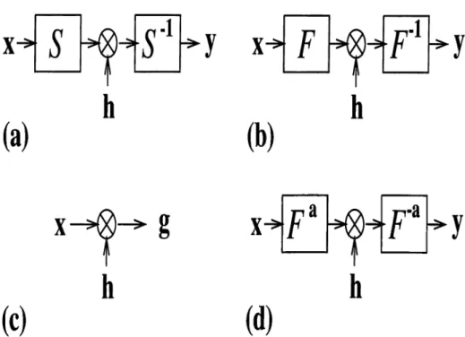
(a)) may also be interpreted as a special case o f single-stage transform domain filtering which is in turn a sub-class o f general linear systems. General single-stage transform domain filtering configuration is shown in Fig. 3.1 (a). According to this configuration, the output is obtained by multiplying the input with a filter function

h

in the transform domain. The overall system is characterized by:

r = S~^AS

(3.1)

where <S is a transform and A corresponds to a multiplication with the filter function

h. T

can be implemented efficiently if the transform

S

has efficient implementation. The time-invariant system is a special case with the transform <S equals to the ordinary Fourier transform (Fig. 3.1 (b)). Other special case may be obtained by using the identity transform (<S = X) and in this case we have the time or space domain filtering for which the output is obtained by simply masking the input with a window function

h

(Fig. 3.1 (c)).

If we choose the transform in (3.1) as the fractional Fourier transform (<S = X"“ ), we obtain the single-stage fractional Fourier domain filter (Fig. 3.1 (d)). In this case the overall system is given by;

Tss

= X " “A X “ (3.2) This configuration interpolates between the time-domain and frequency domain filtering configurations and enables significant improvements in signal restoration and denoising as discussed below [7, 10,

12

].

As a simple application of the single-stage fractional Fourier domain filtering we consider the signal or image restoration problem. In many signal processing applications, signals which we wish to recover are degraded by a known distortion and/or by noise. Then the problem is to reduce or eliminate these degradations. Appropriate solutions to such problems depend on the observation model and the objectives, as well as the prior knowledge available about the desired signal, degradation process and noise. A commonly used observation model is

(a)

(b)

y

h

(c)

g

(d)

F "i

y

Figure

3

.

1

: (a) Single-stage transform domain filtering, (b) Fourier domain filtering, (c) time (space) domain filtering, (d) fractional Fourier domain filtering.

where

Q

is the linear system that degrades the desired signal (may be an image) .x·, and

n

is an additive noise term. The problem is to find an estimation operator represented by the kernel

Ti,

such that the estimated signal

^est — ^^obs minimizes the mean square error defined as:

(3.4)

(3.5) where || · |p denotes a norm and

E[·]

denotes an ensemble average. The classical Wiener filter provides the solution to the above problem when the degradation is time-invariant and the input and noise processes are stationary. The Wiener filter is time-invariant, and can thus be implemented effectively with a multiplicative filter in the conventional Fourier domain with the fast Fourier transform algorithm. For an arbitrary degradation model or non-stationary processes, the classical Wiener filter cannot often provide a satisfactory result. In this case, the optimum recovery operator is in general time-varying and has no fast implementation. However we can use the single-stage fractional Fourier domain filter to improve the performance. This filtering configuration has been studied in detail in [

8

, 10] for

1

-D signals and in [

12

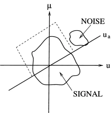
] for 2-D signals and images.

To understand the basic motivation for filtering in fractional Fourier domains, consider Fig.

3

.

2

, where the Wigner distributions of a desired signal and an undesired distortion are superimposed. We observe that they overlap in both the

0

th and

1

st domains, but they do not overlap in the

0

.

5

th domain (consider the projections onto the

«0

= w, ui =

n,

and uo

.5

axes). Although we cannot eliminate the distortions in the space or frequency domains, we can eliminate them easily by using a simple amplitude mask in the

0

.

5

th domain.

We now discuss the optimal filtering problem mathematically. The estimated (filtered) signal a;est is expressed as

^est — (3·^)

=

(3.7)

According to equation 3.7, we first take the ath order fractional Fourier transform of the observed signal Xobs» then multiply the transformed signal with the filter

h

and take the inverse ath order fractional Fourier transform o f the resulting signal to obtain our estimate. Since the fractional Fourier transform has efficient digital and optical implementations, the cost of fractional Fourier domain filtering is approximately the same as the cost o f ordinary Fourier domain filtering. With the above form of the estimation operator, the problem is to find the optimum multiplicative filter function hopt that minimizes the mean-square error defined in equation 3.5.

For a given transform order a, hopt can be found analytically using the orthogonality principle or the calculus of variations [

8

,

10

,

12

]:

.f f

^)A^_a(Uo,

U

U

)

du du

fiopt(w) =

S I

A^o(’^tt) ^)AT_a(U(i, W^).Rioi,globs(^>

^0

(3.8) where the stochastic auto- and cross-correlation functions

u')

and

Rxx^^Xu, u')

can be computed from the correlation functions

Rxx(u,u')

and

Rnn{%u')

(which are assumed to be known).

Th above formulation gives the solution for

1

-D signals. The problem and the solution can be generalized to 2-D signals and images by using both separable and non-separable definitions o f the fractional Fourier transform [12, 24]. When applied to

2

-D signals and images, some form of windowing is necessary before the fractional Fourier transform stages to reduce the boundary artifacts [

12

].

Fractional Fourier domain filtering is particularly advantageous when the distortion or noise is o f a chirped nature. Such situations are encountered in many real-life