Contents lists available atScienceDirect
Performance Evaluation
journal homepage:www.elsevier.com/locate/peva
Markov fluid queue model of an energy harvesting IoT device
with adaptive sensing
C. Tunc
a,
N. Akar
b,*
aNYU Tandon School of Engineering, Department of Electrical and Computer Engineering, Brooklyn, NY, USA bElectrical and Electronics Engineering Department, Bilkent University, Ankara, Turkey
a r t i c l e i n f o
Article history: Received 3 August 2016
Received in revised form 2 December 2016 Accepted 19 March 2017
Available online 31 March 2017 Keywords:
Wireless sensor networks Internet of things Energy harvesting Adaptive sensing Markov fluid queues Risk theory
a b s t r a c t
Energy management is key in prolonging the lifetime of an energy harvesting Internet of Things (IoT) device with rechargeable batteries. Such an IoT device is required to fulfill its main functionalities, i.e., information sensing and dissemination at an acceptable rate, while keeping the probability that the node first becomes non-operational, i.e., the battery level hits zero the first time within a given finite time horizon, below a desired level. Assum-ing a finite-state Continuous-Time Markov Chain (CTMC) model for the Energy HarvestAssum-ing Process (EHP), we propose a risk-theoretic Markov fluid queue model for the computation of first battery outage probabilities in a given finite time horizon. The proposed model enables the performance evaluation of a wide spectrum of energy management policies including those with sensing rates depending on the instantaneous battery level and/or the state of the energy harvesting process. Moreover, an engineering methodology is proposed by which optimal threshold-based adaptive sensing policies are obtained that maximize the information sensing rate of the IoT device while meeting a Quality of Service (QoS) constraint given in terms of first battery outage probabilities. Numerical results are presented for the validation of the analytical model and also the proposed engineering methodology, using a two-state CTMC-based EHP.
© 2017 Elsevier B.V. All rights reserved.
1. Introduction
Wireless Sensor Networks (WSNs) refer to an interconnection of a number of Sensor Nodes (SN) each of which is deployed for the purpose of gathering the sensory information regarding the located environment and disseminating this information across the WSN [1,2]. WSNs target a wide spectrum of applications including indoor/outdoor environment monitoring, target tracking, logistics support, robotics, etc. [3]. WSNs are typically battery-operated and energy management of WSNs is therefore of utmost importance. Most WSNs explored in the literature are short-range multi-hop (mesh) networks where most of the existing research is directed towards networking, routing, and energy efficiency aspects of WSNs [1,2,4]. For relatively longer ranges, mesh architectures are not battery efficient since the nodes need to continuously receive, repeat, and route their neighbors’ Radio Frequency (RF) signals which makes it quite difficult to efficiently manage the energy consumption of SNs [5].
An alternative long-range technology is Low-Power Wide Area Networks (LPWANs) with star topologies, i.e., single-hop connectivity. LPWANs employ sub-GHz unlicensed frequency bands for long-range and low-power communications [6]. LPWANs are promising for IoT (Internet of Things) environments which refer to a network of interconnected things or
*
Corresponding author. Fax: +90 312 2664192.E-mail addresses:[email protected](C. Tunc),[email protected](N. Akar).
http://dx.doi.org/10.1016/j.peva.2017.03.004
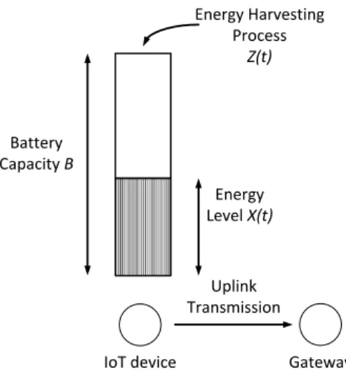
Fig. 1. Illustration of an energy harvesting IoT device.
devices equipped with sensors and/or actuators with wireless communication interfaces [6]. In LPWANs, the IoT devices are one hop away from a unique sink node, named as the gateway, which provides bridging to the IP-based Internet [6]. We refer the reader to [5–8] for various LPWAN technologies including IEEE 802.11ah, LoRa, SigFox, Ingenu, etc. Although there are similarities between WSNs and IoTs, the Internet connectivity requirements of IoTs, strict energy consumption requirements on IoTs, and additionally the size of the population (far larger in IoTs than typical WSNs) appear to be the key differences between them. Although bi-directional communication is possible in most IoT technologies, the mandatory scenario is uplink communications via which end devices occasionally send data to the gateway; this latter scenario being the focus of this paper.
One of the main concerns regarding WSNs has been energy efficiency using various methods aiming at prolonging the lifetime of the individual SNs of the WSN [4,9]. Similarly, there has been recent interest in energy efficiency for IoTs; see [10,11] and the references therein. Deployment of energy harvesting sources on end devices including solar, thermal, electromagnetic, kinetic, or indoor lighting-based sources, has been proposed to address this concern [12–14]. The focus of this paper will be on the energy management of energy harvesting end systems in the LPWAN setting with the end system having direct uplink connectivity to the gateway. The end system in IoTs will be called an IoT device or simply device throughout the paper.
In the current paper, we consider an energy harvesting IoT device illustrated inFig. 1with its rechargeable battery modeled by a single buffer for energy storage. The energy harvesting process Z (t) dictates the instantaneous rate at time t at which the battery is charged/discharged. Positive (negative) values for this rate are representative of energy harvesting (leakage). We assume that Z (t) is governed by a general finite-state CTMC with initial probability vector
α
at time zero. In the device model ofFig. 1, the battery energy process X (t)∈ [
0,
B]
denotes the stored energy at the battery at time t and the capacity limit B represents the maximum amount of energy that the battery can hold. The initial battery level is denoted by u, i.e., X (0)=
u. Similar to the system model envisioned in [15] and [16], when the IoT device decides to sense the environment, it samples the physical quantities of interest, processes this information, forms a data packet, and immediately transmits towards the gateway using the IoT environment. Since the sensing, processing, packetization, and transmission sub-steps are combined into one single step in this model, the system we envision does not need to possess a data buffer to store data packets. For convenience, we call this combined step as sensing. The count process related to the sensing epochs (or the data packet arrival process) is modeled by a non-homogeneous Poisson process with rateλ
(X (t),
Z (t)), also called the adaptive sensing rate, which is allowed to depend on the instantaneous battery level and the state of the harvester process. For the purpose of analytical tractability, we ignore transmission errors and MAC (Medium Access Control) layer retransmissions, or equivalently, we assume that when a data packet is transmitted, it is successfully received by the gateway. The impact of the MAC layer and transmission errors are left for future research. In our model, the energy dissipated for one single data packet transmission (denoted by S) is assumed to be exponentially distributed with mean E[
S]
. We assume that this quantity captures the energy dissipated for all the four sub-steps. Since the time scales of operation for the slower EHP and the relatively rapid packet transmission process are quite different, we assume without loss of generality that the packet transmission takes place instantaneously resulting in an abrupt energy drop by an amount of S each time a data packet gets to be transmitted. Temporary battery outage is said to occur at time t when the buffer is first depleted, i.e, X (t)=
0, after which the device would not be able to fulfill its functionalities, i.e., temporary IoT service interruption, until the device finds a chance again to harvest energy. As the QoS constraint, we propose in this paper to use the finite-horizon outage probability which is defined as the probability of first battery outage within a given time horizon H.The main goal of this paper is to first analytically obtain the finite-horizon battery outage probability as a function of all system model parameters. Note that this probability depends on the initial buffer level u, initial probability vector
α
ofthe EHP, and the time horizon H. For this purpose, we propose to construct a Multi-Regime Markov Fluid Queue (MRMFQ) model for the energy harvesting IoT device; see [17] and [18] for a detailed study of MRMFQs. We note that numerically stable and computationally efficient algorithms are available in the literature for the steady-state solution of MRMFQs [18]. The reference [19] proposes a method to compute the finite-horizon ruin probabilities for a risk problem with surplus-dependent premiums, claim arrivals modeled by a Markovian arrival process, and PH-type claim sizes with a matrix-analytical algorithm. Such ruin probabilities are given in terms of the steady-state probability mass accumulations of an associated MRMFQ at certain levels [19]. Similar to the findings of [19], we express in this paper the finite-horizon battery outage probabilities as the ratio of certain steady-state probability mass accumulations of our proposed MRMFQ model. The second goal of this paper is to use this analytical method as an instrument to find the optimum transmission policies regarding the choice of the sensing rate function
λ
(X (t),
Z (t)) meeting the QoS constraint with the purpose of maximizing the average long-term sensing rate. Towards the second goal and for tractability purposes, we focus our attention to the commonly used two-state CTMC model for the EHP and threshold-based transmission policies in which the instantaneous sensing rateλ
(X (t),
Z (t)) is eitherλ
minorλ
max> λ
min, depending on whether X (t) is above or below a given thresholdwhich is allowed to depend on the current state of the EHP. This generality in analysis allows us to compare various non-adaptive/adaptive sensing policies. MRMFQs have already been used to model the energy process of a rechargeable battery in a few studies. In the most related work of [20] and [21], a two-regime two-state Markov fluid queue model for a rechargeable battery is studied with a single battery level threshold. Below the threshold, a power-save mode is entered and the rate of discharge is decreased in [20,21]. The main contributions of the current paper are:
•
The power discharge is modeled more explicitly in our work (than the model presented in [20] and [21]) by abrupt drops stemming from sensing events which is more realistic in IoT environments.•
A threshold is defined for each state of the EHP, i.e., state-dependent threshold policy, enabling the model to be more general than the one studied in [20] and [21]. This generalization will be shown to be advantageous especially for short time horizons or slower EHPs through numerical examples.•
The mathematical formulation developed in this paper allows the EHP to be modeled with a CTMC with arbitrary number of states and with arbitrary number of thresholds.•
In [20,21], an expression for the Laplace transform of the battery life’s probability density function is first obtained which is then inverted numerically for particular instances. However, obtaining this Laplace transform as in [20] requires symbolic mathematical operations (the equations were implemented in the symbolic math package Math-ematica in [20]), which does not scale well to large systems. In the current paper, we provide a matrix-analytical approach that saves one from obtaining Laplace transforms and their inversion altogether. This allows one to very rapidly obtain battery outage probabilities for a given set of design parameters and subsequently repeat the analysis as a function of these parameters for the purpose of parameter optimization.•
In terms of the numerical method to solve the arising MRMFQ, we use the method described in [18] but the proposed MRMFQ model for energy harvesting is unique to the current paper but has commonalities with the MRMFQ model described in [19] for computing ruin probabilities. In our work, the inter-event times are exponentially distributed with parameter dynamically adjusted on the battery level whereas the premiums collected by an insurance company is dynamically adjusted in [19] according to the instantaneous surplus. Moreover, we propose an expression for the average sensing rate in the current paper, the counterpart of which is not studied in [19].The paper is organized as follows. In Section2, related work on energy management of energy harvesting SNs and IoTs are given as well as a brief introduction to MRMFQs and their applications to modeling energy harvesting devices. The computational procedure for finding the battery outage probabilities for the system ofFig. 1is presented in Section3. In Section 4, the proposed analytical technique is validated using simulations and moreover the proposed engineering methodology to find the optimum sensing rate function is presented for a wide range of system parameters. Finally, we conclude.
2. Related work
We now present the related work on energy management of energy harvesting devices. Then, we provide a brief overview of fluid queues and MRMFQs as well as the related work on their applications to modeling energy harvesting devices. 2.1. Energy management in energy harvesting devices
There have been quite a few recent studies on the energy management problem in energy harvesting devices; see [22] for a recent review. A subset of these studies concentrate on an optimization problem on the basis of the availability of the off-line knowledge of energy and data arrivals at the device, which is most commonly referred to as the off-off-line problem in the literature. As a representative example, the reference [23] studies the offline problem in a SN with one data queue storing data arrivals, and another queue storing energy harvested from the environment, and obtains a globally optimal offline scheduling policy with the purpose of minimizing transmission completion time for several data packet arrival scenarios. On the other hand, problems involving systems with both data and energy arrivals modeled by a random process are referred to as on-line problems. On-line problems are more realistic since it is not appropriate to have a deterministic a-priori known
model for the Energy Harvesting Process (EHP) in most IoT settings. For the particular example of solar sources, the amount of harvested solar energy may vary depending on daily conditions such as temperature, amount and size of clouds, etc. The EHP is often characterized with stationary discrete-time Markovian models stemming from their amenability to analysis [24–26]. The reference [27] investigates how well six types of discrete distributions, namely discrete uniform, geometric, transformed geometric, Poisson, transformed Poisson, and two-state discrete Markovian, fit to the real-world solar data. Alternative CTMC models of EHPs are proposed in [28] and [29]. We focus in this paper on the on-line problem and in particular CTMC-based EHP models due to the natural asynchronous operation of the IoT devices.
The existing work related to the on-line problem involves the development of energy management policies for SNs or IoT devices so as to improve the performance of the device in a certain statistical sense. In [15], the authors model the ambient energy supply as a two-state discrete-time Markov chain comprising a good and a bad state, and assume a finite capacity constraint on the basis of which they propose near-optimal transmission policies in terms of the average long-term importance of the reported data. The reference [30] seeks to maximize the long-term average transmission rate while considering an additional data queue and the entire system is modeled with a two-dimensional discrete-time Markov chain whose states correspond to the joint energy and data queue levels. The work in [31] formulates an optimization problem to obtain sensing and transmission policies with the problem constraints being the probabilities that the data buffer gets full or the battery depletes. A related work [32] obtains energy management policies which minimize a linear combination of the mean queue length and the mean data loss rate. In [33], a two-dimensional random walk is proposed for modeling a device for which the data and energy arrivals are modeled by random processes. In particular, when the device stores a given number of energy packets, then it can send a data packet [33]. Adapting the sensing rate (the rate at which the IoT device gathers data from the environment), also known as adaptive duty cycling, is one of the on-line strategies to enhance the throughput performance and the lifetime of an IoT device [34]. The reference [35] studies a model-free approach to adaptive duty cycling using techniques from adaptive control theory whereas [34] presents a method in which the statistical model is available. In [36], the authors formulate an optimization problem to obtain the optimal duty cycle by taking into account the harvested energy with the constraints being the latency and loss probability of the packets that are queued in a finite buffer before being transmitted. The work in [37] compares two policies that adjust sensing epochs and make sensing decisions in order to increase the long term average sensing performance. In the first policy, sensing events are periodic and take place if there is enough energy in the battery or otherwise skipped, which is the optimal policy for an infinite-size battery whereas in the second policy, time between two consecutive sensing events also depends on the battery level and is adjustable. The scope of the current paper is the on-line problem, and in particular the adaptive sensing mechanism using a CTMC-based stochastic model for the EHP.
2.2. Multi-regime Markov fluid queues
In fluid queue models, a fluid acts as the input to and output of a buffer. In particular, Markov Fluid Queues (MFQ) of first-order are described by a joint Markovian process (X (t)
,
Z (t)) where X (t) represents the buffer level and Z (t) is an underlying finite state-space continuous-time Markov chain that determines the drift, i.e., the rate at which the buffer content X (t) changes. The process Z (t) is called the background (or modulating) process of the MFQ. The reference [38] studies MFQs with infinite queue sizes using a spectral expansion approach whereas [39] extends this analysis to finite queue sizes. Second-order MFQs (also known as Markov modulated diffusion processes) generalize first-order MFQs by using Brownian motion modulated by a CTMC [40]. In the absence of modulation, this process is called a diffusion process which has many applications in the analysis of computer systems [41].MRMFQs are generalizations of MFQs by partitioning the buffer space into a finite number of non-overlapping intervals called the regimes (or layers) of the MRMFQ [17,18,42,43]. MRMFQs are also called threshold, level-dependent, multi-layer, or feedback MFQs, in the literature. In MRMFQs, the infinitesimal generator of the background CTMC as well as the drift into the buffer depend on the regime at which the buffer level resides. The material below for the brief description of MRMFQs and their notation is based on [18]. For an MRMFQ, a buffer with finite size B
< ∞
is partitioned into K>
1 regimes with the boundaries 0=
T(0)<
T(1)< · · · <
T(K−1)<
T(K )=
B. If T(k−1)<
X (t)<
T(k), the system is said to bein regime k at time t. Let X (t)
∈ [
0,
B]
and Z (t)∈ {
0,
1, . . . ,
N−
1}
denote the buffer content and the background process, respectively, at time t as in ordinary MFQs. We denote the infinitesimal generator and drift matrices associated with regime k by Q(k)and R(k), respectively, for 1≤
k≤
K . The regime-k drift matrix R(k)is the diagonal matrixR(k)
=
diag(r0(k),
r1(k), . . . ,
rN(k)−1),
where ri(k)is the net drift of the buffer at state i and regime k. Note that Q(k)and R(k)are fixed within a given regime. Similar to Q(k)and R(k), we defineQ
˜
(k)andR˜
(k)as the infinitesimal generator and drift matrices associated with the boundary T(k)for0
≤
k≤
K , where the drift of state i at the boundary T(k)is denoted byr˜
(k)i . We define the joint probability density function
(pdf) vector f(k)(x) for regime k when T(k−1)
<
x<
T(k)as follows:fi(k)(x)
=
lim t→∞ d dxPr{
X (t)≤
x,
Z (t)=
i}
,
(1) f(k)(x)=
[
f0(k)(x) f1(k)(x). . .
fN(k)−1(x)]
.
(2)Similarly, the steady-state probability mass accumulation vector c(k)is defined for each boundary point T(k)as follows: ci(k)
=
lim t→∞Pr{
X (t)=
T (k),
Z (t)=
i}
,
(3) c(k)=
[
c0(k) c1(k). . .
cN(k)−1]
.
(4)Based on [18], the following set of differential equations holds for the joint pdf vector: d
dxf
(k)(x)R(k)
=
f(k)(x)Q(k),
(5)with a set of boundary conditions to be satisfied also given in [18] which proposes a numerically stable and efficient algorithm to find the per-regime joint pdf vector f(k)(x) and the per-boundary mass accumulation vector c(k). This algorithm requires an
ordered Schur decomposition and a pair of Sylvester equations for each regime, and the solution of a linear matrix equation of at most size N(2K
+
1). The computational complexity of the proposed algorithm can be reduced toO(N3K ) on the basisof the observation that the linear matrix equation is in block tridiagonal form [44].
There have been a number of studies that use diffusion and/or MFQ-based queuing models for energy harvesting sensor nodes. A two-regime two-state Markov fluid queue model for a rechargeable battery with a power save mode is studied in [20,21]. The reference [45] investigates a wireless node powered by multiple batteries each of which is modeled by a MRMFQ but the focus has been on the mean node lifetime rather than the battery outage probability. The reference [46] presents a diffusion model for a battery-operated SN to take into account the fluctuations in the amount of energy extracted from the environment. In [47], the energy buffer of a node is modeled as a G/G/1 queue which is then analyzed by the diffusion approximation for the time-dependent behavior of the buffer. An MFQ model is proposed in [48] which captures data transmission together with energy expenditure/replenishment processes in the context of a home gateway system serving a number of IoT devices using Bluetooth low energy with wireless energy transfer capability.
3. Risk-theoretic MRMFQ model
For mathematical analysis, a connection is established in this section between ruin probabilities in risk theory and battery outage probabilities in energy harvesting IoT devices. In risk theory, the ruin problem is described through an insurance company which is exposed to an incoming cash flow in the form of premiums and an outgoing cash flow in the form of claims, the arrival epochs and sizes of claims being modeled by various stochastic processes in the literature; see [49] and the references therein. For an insurer with initial surplus, the ultimate ruin probability is the probability that the insurer’s surplus level eventually falls below zero, i.e., the insurance company goes bankrupt [49]. In most practical scenarios, it is crucial to know about the probability of the surplus level falling below zero within a given finite time horizon, called the finite-horizon ruin probability [50]. The role of premiums (claims) in risk theory will be shown in this paper to be played by energy harvesting (sensing) in energy harvesting IoT devices. Consequently, the counterpart of ruin probabilities turns out to be battery outage probabilities, both within a given time horizon. Recently, [19] proposed a Multi-Regime Markov Fluid Queue (MRMFQ) model to find the finite-horizon ruin probabilities for an insurance company with surplus-dependent premiums, claim arrivals modeled by a Markovian arrival process, and PH-type claim sizes with a matrix-analytical algorithm. With the proposed technique of [19], one can express the finite-horizon ruin probability in terms of the steady-state probability mass accumulations of the associated MRMFQ at certain levels. On the other hand, steady-state distribution of an MRMFQ can be obtained using computationally efficient and numerically stable matrix-analytical algorithms proposed in [18]. In this section, we extend the method proposed in [19] to compute the finite-horizon battery outage probabilities of the system depicted inFig. 1for a specific choice of the sensing rate function
λ
(X (t),
Z (t)). Subsequently, an expression will be derived for the average sensing rate which will be essential in the engineering methodology we introduce so as to obtain the optimum sensing rate function meeting the QoS requirement detailed in Section1. For notation, In, 1n×m, and 0n×mdenote an identity matrix of size n, a matrix of ones of size n×
m, and a matrix of zeros of size n×
m, respectively.3.1. System model
The Energy Harvesting Process (EHP) Z (t)
∈ {
0,
1, . . . ,
N−
1}
is governed by an N-state CTMC with infinitesimal generator denoted by Q . We refer to the states of the energy harvesting process as the harvester states. When the EHP resides in state i, the harvester output power level is denoted by pi, for 0≤
i≤
N−
1. Accordingly, we define the matrixP
=
diag(p0,
p1, . . . ,
pN−1). A fixed leakage rate from the battery is assumed and denoted by lb. Subsequently, we define thenet power matrix D
=
P−
lbIN=
diag(d0,
d1, . . . ,
dN−1), where di=
pi−
lbdenotes the net rate of change of the storedenergy in the battery when the EHP resides in state i.
We focus on the particular case when the sensing rate function
λ
(X (t),
Z (t)) is a piece-wise constant function of the instantaneous battery level X (t), i.e., the sensing rate depends only on Z (t) when X (t) resides between two boundaries. For this purpose, we define the regime boundaries 0=
T(0)<
T(1)< · · · <
T(J)=
u< · · · <
T(K )=
B, where u andB are the initial battery level and battery capacity, respectively. The battery is said to reside in regime k at time t when T(k−1)
<
X (t)<
T(k). We denote the sensing rate in harvester state i and regime k byλ
i(k) for 0
≤
i≤
N−
1 and 1≤
k≤
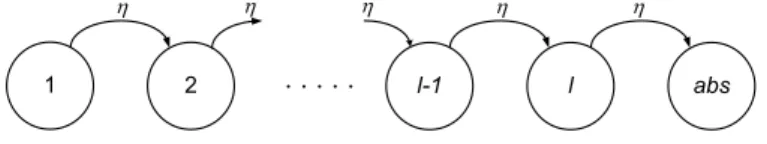
K .Fig. 2. l-level Erlangization of the horizon H.
The system starts to operate with initial battery level u and in an harvester state according to a given initial probability vector
α = [α
0α
1. . . α
N−1]
whereα
i=
Pr{
Z (0)=
i}
. Whenever Z (t) is in state i, the energy in the battery changes withrate di
=
pi−
lb. When pi<
lb, the energy buffer is drained at rate lb−
pi. When T(k−1)<
X (t)≤
T(k), a sensing eventoccurs in the interval (t
,
t+
∆t) with probabilityλ
i(k)∆(t)+
O(∆t) whereo(∆∆tt)→
0 as∆t→
0. A sensing event leads toan immediate battery energy drop with amount S which is exponentially distributed with mean E
[
S]
. Obviously, the battery level X (t) can not be negative. The time of battery outage denoted byτ
(u, α
) is given byτ
(u, α
)=
inf{
t>
0:
X (t)=
0}
,
(6)and the finite-horizon battery outage probability before the so-called horizon value H denoted by
ψ
(u, α,
H) is then given byψ
(u, α,
H)=
Pr{
τ
(u, α
)<
H}
.
(7)The average sensing rate
λ
avgrepresents the average number of transmitted data packets (i) in the time interval[
0,
H]
if nooutage occurs within H, or (ii) in the interval
[
0, τ
(u, α
)]
in caseτ
(u, α
)<
H. 3.2. MRMFQ modelIn order to model the deterministic time horizon H in our MRMFQ model, we use Erlangization which refers to approximating a deterministic quantity by an Erlang distribution of sufficiently high order for analytical tractability; see for example [50] that employs Erlangization to approximate the deterministic time horizon in the risk theory context. In this paper, we employ l-stage Erlangization to model the deterministic horizon H as depicted inFig. 2for various values of the parameter l. The state labeled as abs refers to the absorbing state representing the horizon expiration and
η =
l/
H is the transition rate from one Erlang stage to the next one. Starting operation at the first stage at time zero, the time to reach the abs stage is then Erlang-l distributed with mean H. Clearly, as l→ ∞
, the Erlang-l distribution converges to a Dirac delta function located at H. We define the following Erlang-l sub-generator THand the vector TH0to be used in the MRMFQ modelwe propose: TH
=
⎡
⎢
⎢
⎢
⎢
⎣
−
η
η
−
η
η
... ...
−
η
η
−
η
⎤
⎥
⎥
⎥
⎥
⎦
,
T0 H= −
TH1l×1.The state-space of our MRMFQ model is now described. First, we need l replicas of each harvester state, which are represented by the pair (i
,
j) for 0≤
i≤
N−
1 and 1≤
j≤
l, resulting in a total number of Nl so-called idle states, since there is no data transmission in these states. As packets being transmitted, there should be a reduction in the battery level. For this purpose, we need a transmission-mode replica of the idle state (i,
j) denoted by (i,
j)* and these Nl replicas will be referred as the transmitting states. A sensing event forces the system to move from state (i,
j) to state (i,
j)*. On the other hand, we move from (i,
j)* to (i,
j) upon the completion of a transmission unless battery outage occurs. These two sets of states are indeed sufficient to describe the long-term evolution of the battery energy process X (t). However, as far as the battery outage probabilities are concerned, the evolution of X (t) beyond the horizon, i.e., t>
H is not needed at all. Therefore, when the time horizon H is reached, we propose to bring the battery energy to its initial value u and the EHP process to its initial state according to the initial probability vectorα
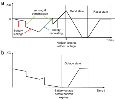
and let the battery energy process evolve again. When this process repeats itself, we obtain an em-bedding of the whole sequence of battery energy processes into one single trajectory of a specially constructed MRMFQ. With the aim of constructing this MRMFQ, we propose to use three additional states, namely Outage (O), Reset (R), and Good (G) states. We describe the use of these states inFig. 3which depicts two sample paths for the battery energy process which is re-set to its initial values each time the horizon is reached. Note that within the horizon H, either of the two events would occur:•
No battery outage: For this event, time expires before the horizon without the battery level hitting zero. We introduce the G and R states to describe the behavior of the battery level in this case. As the horizon expires, the battery level is decreased down to zero (during the G state) and then increased up to the initial level u (in the R state); seeFig. 3(a).•
Battery outage: The battery level hits zero before the horizon. In this case, the O state is used to initialize the batteryFig. 3. Sample paths for (a) no battery outage, (b) battery outage, within a finite horizon H.
In either case, with the battery level set to u, the system transits into one of the first Erlang states (i
,
1), 0≤
i≤
N−
1, according to the initial probability vectorα
and the cycle starts over. Note that inFig. 3, abrupt falls of the battery level represent data transmission and battery leakage (energy harvesting) is shown by a negative (positive) slope.The trajectories inFig. 3can not be described by an MRMFQ yet due to the discontinuities. Therefore, we propose to reduce the energy level at a finite rate of pT as opposed to abrupt drops. For this purpose, we choose scalar parameters pT and
β
such that the mean dissipated energy for one packet transmission E
[
S]
equals the product pT/β
. Consequently, each time apacket gets to be transmitted, the battery level is allowed to reduce at a rate of pTfor an exponentially distributed amount of
time with parameter
β
leading to an exponentially distributed eventual energy drop with mean E[
S]
. With this modification (does not lead to any inaccuracy as will be shown in the sequel), the trajectories inFig. 3can be expressed as an MRMFQ for which we order the states as (i) O state, (ii) R state, (iii) G state, (iv) Nl idle states enumerated lexicographically, (v) Nl transmission states enumerated lexicographically. With this state space, we are now ready to describe the MRMFQ model which is a translation of the sample paths provided inFig. 3into an MRMFQ that uses the regime boundaries T(k),
0≤
k≤
K . Therefore, in the proposed MRMFQ model, the regime-k generator matrix is expressed asQ(k)
=
⎡
⎢
⎢
⎢
⎣
0 0 0 01×Nl 01×Nl 0 0 0 01×Nl 01×Nl 0 0 0 01×Nl 01×Nl 0Nl×1 0Nl×1 1N×1⊗
TH0 IN⊗
TH+
(
Q−
Λ(k)) ⊗
Il Λ(k)⊗
Il 0Nl×1 0Nl×1 0Nl×1β
INl−
β
INl⎤
⎥
⎥
⎥
⎦
.
The boundary-k generator matrixQ
˜
(k)=
Q(k)for k∈ {
1,
2, . . . ,
J−
1,
J+
1, . . . ,
K}
. The boundary-J generator is slightlydifferent as given below:
˜
Q(J)=
⎡
⎢
⎢
⎢
⎣
−
1 0 0α ⊗
e1 01×Nl 0−
1 0α ⊗
e1 01×Nl 0 0 0 01×Nl 01×Nl 0Nl×1 0Nl×1 1N×1⊗
TH0 IN⊗
TH+
(
Q−
Λ(J)) ⊗
Il Λ(J)⊗
Il 0Nl×1 0Nl×1 0Nl×1β
INl−
β
INl⎤
⎥
⎥
⎥
⎦
,
where e1denotes a row vector of zeros of size l except for a one in the first position. The boundary-0 generator is given
below:
˜
Q(0)=
⎡
⎢
⎢
⎢
⎣
0 0 0 01×Nl 01×Nl 0 0 0 01×Nl 01×Nl 0 1−
1 01×Nl 01×Nl 1Nl×1 0Nl×1 0Nl×1−
INl 0Nl×Nl 1Nl×1 0Nl×1 0Nl×1 0Nl×Nl−
INl⎤
⎥
⎥
⎥
⎦
.
The regime-k and boundary-k drift matrices of the proposed MRMFQ are given as follows: R(k)
=
{
diag(1,
1, −
1,
D⊗
Il, −pTINl),
1≤
k≤
J,
diag(−
1, −
1, −
1,
D⊗
Il, −pTINl),
J<
k≤
K.
(8)˜
R(k)=
⎧
⎪
⎪
⎨
⎪
⎪
⎩
R(k),
k̸∈ {
0,
J,
K}
,
max(0,
R(1)),
k=
0,
diag(0,
0, −
1,
D⊗
Il, −pTINl),
k=
J,
min(0,
R(K )),
k=
K,
(9)where the max and min are element-wise operators. With the way the MRMFQ is constructed, note that the amount of time spent in the O and R states during each visit to these two states possess the same distribution. This observation holds also for the time spent in these two states restricted to x
=
u. Consequently, the finite-horizon battery outage probabilityψ
(u, α,
H) can be written asψ
(u, α,
H)=
c (J) O cO(J)+
c(J)R,
(10)where cR(J) and cO(J) as the probability mass accumulations of the proposed MRMFQ at the boundary J in states R and O, respectively. Subsequently, we propose to use the method described in [18] to solve for the steady-state distribution (in particular the quantity given in(10)) of the specially constructed MRMFQ with 2Nl
+
3 states and K regimes. Note that the computational complexity of the entire process isO(N3l3K ) [51].3.3. Engineering methodology
By solving the mathematical model described above, we now derive an expression to calculate the average sensing rate
λ
avg. Subsequently, we study various adaptive sensing rate policies to maximize the average sensing rate where the systemrequirement is the finite-horizon outage probability given in(10)being less than a given desired probability
ψ
T. For thepurpose of reducing the number of decision variables for computational tractability, the sensing rate
λ
i(k) is allowed to takeeither a minimum or a maximum value, denoted by
λ
minandλ
max, respectively. The optimization problem we deal with canbe written as:
maximize
λ
avgsubject to
ψ
(u, α,
H)< ψ
T,
λ
i(k)=
λ
minorλ
max(11)
for 1
≤
k≤
K . Intuitively, when the battery level is close to zero, the rate should be set toλ
minto avoid battery outage.Similarly, the IoT device should sense the environment with rate
λ
maxwhen the battery is almost fully charged to provideenough space in the battery for new energy arrivals. This leads us to investigate a threshold-based structure for
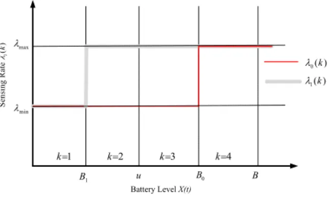
λ
i(k). In thisstudy, we assume a two-state EHP with two harvester states 0 and 1 and the thresholds for these states are denoted by B0
and B1, respectively. Since we let each state have its own threshold, we refer to this policy as the State-Dependent Threshold
Policy (SDTP). SDTP being employed for a two-state energy harvesting process results in a 4-regime MFQ. Together with the boundary points at T(0)
=
0, T(J)=
u and T(K )=
T(4)=
B, we have two more boundary points each of which correspondsto the threshold of one harvester state. For instance, if B1
<
u<
B0, we have T(1)=
B1, T(2)=
u and T(3)=
B0. Similarly, ifB1
<
B0<
u, the boundary points can be written as T(1)=
B1, T(2)=
B0and T(3)=
u, and so on. As an example, the SDTPpolicy for the case B1
<
u<
B0<
B is illustrated inFig. 4. Note that two or more boundary points may coincide, which willnot have any adverse effect on the solution methodology. Similar to the power-save mode proposed in [20], we also define the Single Threshold Policy (STP) for which there is a single threshold for the battery level regardless of the harvester state, i.e., B0
=
B1. Clearly, STP can be modeled with a 3-regime MRMFQ. We denote the steady-state joint pdf and probability massaccumulations of the idle state (i
,
m) in regime k by f(i(k),m)(x) and at boundary point T(k)by c(k)(i,m), respectively. To calculate the
average sensing rate
λ
avg, we also denote the normalized steady-state joint pdf and probability mass accumulationsˆ
f(i(k),m)(x)andc
ˆ
(i(k),m)for idle states. Since O, R, and G are auxiliary states which are defined to calculate the outage probability, we censor these states towards the calculation of the average sensing rate. Transmitting states also need to be censored since transmissions are modeled as abrupt falls of the instantaneous battery level. Finally, since probability mass accumulations at zero occur due to battery outage, we also censor them. Subsequently, we write the normalized the steady-state joint pdfˆ
f(i(k),m)(x) as:ˆ
f(i(k),m)(x)=
f (k) (i,m)(x)∑
1 i=0∑
l m=1(
∑
K k=1∫
T(k)− T(k−1)+f (k) (i,m)(x)dx+
∑
K k=1c (k) (i,m))
·
(12)Fig. 4. Sensing rateλi(k) for the case B1<u<B0<B.
The quantitiesc
ˆ
(k)(i,m)can be obtained similarly. The generalization of these equations to N-state EHPs is straightforward. With these normalized quantities, one can calculate the average sensing rate as follows:λ
avg=
1∑
i=0λ
minPr{
Z (t)=
i,
X (t)≤
Bi} +
λ
maxPr{
Z (t)=
i,
X (t)>
Bi}
=
1∑
i=0 l∑
m=1⎡
⎣
λ
min Ki∑
k=1(
∫
T(k)− T(k−1)+ˆ
f(i(k),m)(x)dx+ ˆ
c(k)(i,m))
⎤
⎦
+
1∑
i=0 l∑
m=1⎡
⎣
λ
max K∑
k=Ki(
∫
T(k)− T(k−1)+ˆ
f(i(k),m)(x)dx+ ˆ
c(i(k),m))
⎤
⎦
(13)where Ki(Ki) is the value of k such that T(k)
=
Bi(T(k−1)=
Bi). With the expressions derived for the battery outage probabilityand average sensing rate in terms of the steady-state solution of a certain MRMFQ with 2Nl
+
3 states, one can solve for the outage probabilities as a function of the pair (B0,
B1). The particular values of this pair that yield the largest average sensingrate among those that yield
ψ
(u, α,
H)< ψ
Tare to be chosen as the optimum pair of threshold parameters.4. Numerical examples
4.1. Model parameters
Throughout this section, the units of power and energy are to be taken as mW and mWh, respectively. The time unit is set to hours; however the unit for the horizon parameter H is set to months for convenience. In [13], properties of various rechargeable battery technologies are investigated including two commonly used Nickel Metal Hydride (NiMH) and Lithium-based batteries. Although Lithium-based batteries outperform NiMH batteries in several aspects such as energy and power densities, charging efficiency and self-discharge rate, recharging Li-based batteries requires relatively sophisticated circuits. In numerical examples, we use a NiMH battery model whose self discharge rate, charging efficiency, and capacity are 30%/month, 66% and 3000 mWh, respectively, yielding the choice lb
=
1.
25 in our stochastic model. We use the firstorder radio model given in [52] assuming a d4energy loss as a function of distance d. According to this model, the IoT device
consumes
ETx(k
,
d)=
k(Eelec+
ϵ
ampd4) (14)of energy to transmit a k-bit packet over a distance d. Eelecand
ϵ
ampare the amounts of energy that the transmitter circuitryand amplifier consume per bit, respectively. In the examples, we set Eelec
=
50 nJ/bit,ϵ
amp=
100 pJ/bit/m4, d=
100 mand we assume exponentially distributed packet sizes with mean 1000 bytes giving rise to E
[
S] ≈
22.
222 mWh to transmit one packet on the average. We also set pT=
10 andβ =
0.
45. We assume that the IoT device is equipped with a solar cellof size 37
×
33 mm2as in [53,54]. As discussed in [13], we assume 100 mW/cm2of available energy and 15% conversionefficiency. With 66% charging efficiency of the NiMH battery, 120 mWh of energy can be stored in one hour. According to the data records of solar irradiance reported in [55], the average daily stored energy is 483 mWh for the solar cell model used in that study. Motivated by the studies including [25] and [56], we employ a two-state EHP (1 for harvesting and 0 for no harvesting). Energy is stored in the battery with a power of 120 mW (p1) and 0 mW (p0) for exponentially distributed time
(a) u=750. (d) u=750.
(b) u=2000. (e) u=2000.
(c) u=2750. (f) u=2750.
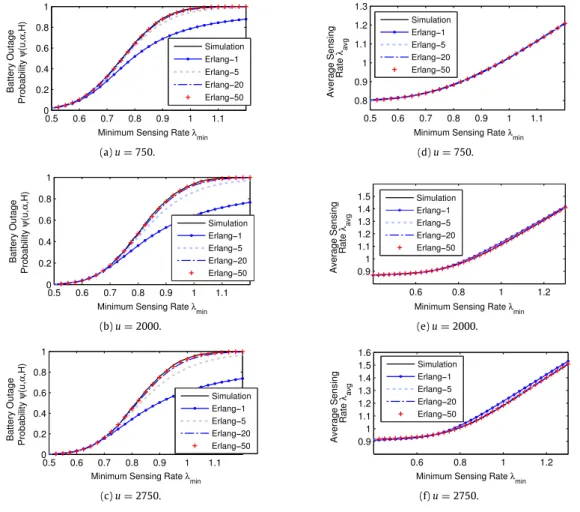
Fig. 5. Battery outage probabilityψ(u, α,H) and average sensing rateλavgin (a), (b), (c) and (d), (e), (f), respectively, as functions ofλminfor H=1,λmax=4,
B1=1500, B0=2500 and u=750,2000 and 2750.
intervals with means 1 and 5 h, respectively. This results in a daily stored energy of 480 mWh which is consistent with the measurements in [55]. For this model, one can write the Q , P, and D matrices as:
Q
=
[−
1/
5 1/
51
−
1]
,
P=
diag(0,
120),
and D
=
P−
lbIN=
diag(−
1.
25,
118.
75). Note that the steady-state probability vector of Q is given byπ = [
5/
6 1/
6]
satisfyingπ
Q=
0.4.2. Example I - Validation
In the first example, we verify the accuracy of the outage probability and average sensing rate expressions derived in Section3. For this purpose, the system is simulated for 105time cycles where a time cycle refers to a single horizon for each
of which we keep track of whether outage has occurred or not, and additionally the number of overall transmitted packets. As the system parameters, we set H
=
1,λ
max=
4, B1=
1500, and B0=
2500, and varyλ
minand compare the resultingoutage probabilities and average sensing rates with the simulation results inFig. 5(a), (b), (c) and (d), (e), (f), respectively, for u
=
750,
2000,
2750. For all of the following examples, we setα = [
5/
6 1/
6]
unless otherwise stated. We observe that as the number of Erlangization levels l increases, the analytical results for
ψ
(u, α,
H) converge to the simulation results, while the average sensing rate seems to be less sensitive to the particular choice of l. A remarkable accuracy is obtained with the choice of l=
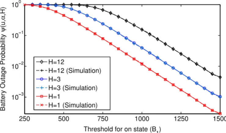
50 (requires a computation time of approximately 0.6 sec. with MATLAB running on a notebook using an Intel Core i5-3210M Processor and a RAM of 8 GB for one problem instance) for both performance metrics. Therefore, we set l to 50 for the remaining examples.InFig. 6, the outage probability is depicted as a function of B1when B0is fixed to 1500 and H
=
1,
3,
12. The otherFig. 6. Battery outage probability as a function of B1for H=1,3,12 and u=3000,λmin=0.4,λmax=10,α = [5/6 1/6].
Fig. 7. Battery outage probability as a function ofα = [(1−α1)α1]for u=100,200,300,400,500 andλmin=0.5,λmax=4, H=1, B0=2000, B1=1000. The notation (S) is used to indicate simulation results, others being analytical results.
overlap with the simulation results. We also compare the analytical results with simulations for various values of the initial probability vector
α
and u=
100,
200,
300,
400,
500. We setλ
min=
0.
5,λ
max=
4, H=
1, B0=
2000, B1=
1000 andα = [
(1−
α
1)α
1]
and varyα
1from 0 to 1. As illustrated inFig. 7, the initial harvester state is more important for relativelylower values of the initial battery level u. Again, we observe that the analytical results are in line with simulations.
For validation purposes, we also investigate the case in which a third moderate sensing rate
λ
modsatisfyingλ
min< λ
mod<
λ
maxis introduced which results in two thresholds for each state and four thresholds in total. We denote the thresholds ofstate i by Bi,1and Bi,2for i
=
1,
2 such that the sensing rateλ
i(k) is given by the following expression:λ
i(k)=
{
λ
min
,
X (t)≤
Bi,1,
λ
mod,
Bi,1<
X (t)≤
Bi,2,
λ
max,
X (t)>
Bi,2.
As the other system parameters, we set
λ
min=
0.
4,λ
mod=
2,λ
max=
10, B0,1=
1500, B0,2=
2250, B1,1=
500,B1,2
=
1250, u=
B=
3000,α = [
5/
6 1/
6]
and tabulate the analytical and simulation results for the finite-horizonbattery outage probability
ψ
(u, α,
H) and average sensing rateλ
avg for H=
1,
3,
6,
9,
12 inTable 1. We also provide 98%confidence intervals for
ψ
(u, α,
H) in the simulation results. We observe that the simulation and analytical results match for this four-threshold model as well.4.3. Example II - Fixed Sensing Rate Policy (FSRP)
Let us now assume a Fixed Sensing Rate Policy (FSRP) for which the sensing rate
λ
(X (t),
Z (t)) does not depend on X (t) or Z (t) and equalsλ
. For a given desired outage probabilityψ
T, we define the maximum attainable fixed sensing rateλ
*calledthe limit-sensing rate which meets the outage probability constraint. In this case, the MRMFQ possesses two regimes with T(0)
=
0<
T(1)=
u≤
T(2)=
B . For this example, we assume that the battery is initially fully charged, i.e., u=
B=
3000, andthe horizon H is varied from 1 to 24 months. For other parameters being fixed, one can easily obtain the value of
λ
*by binarysearch. The limit sensing rate
λ
*is depicted inFig. 8as a function of the horizon H for four different values ofψ
Table 1
Comparison of analytical and simulation results forλmin=0.4,λmod=2,λmax=10, B0,1=1500, B0,2=2250, B1,1=500, B1,2=1250, u=B=3000, α = [5/6 1/6]and H=1,3,6,9,12.
H ψ(u, α,H) λavg
Analytical Simulation Analytical Simulation
Result Result 98% Conf. Int. Result Result
1 0.0135 0.0134 ±0.0007 0.9677 0.9677 3 0.0499 0.0503 ±0.0014 0.8867 0.8869 6 0.1019 0.1021 ±0.0019 0.8664 0.8665 9 0.1510 0.1514 ±0.0022 0.8597 0.8597 12 0.1974 0.1977 ±0.0025 0.8563 0.8565 Table 2
Execution time of the MATLAB code (in seconds) to obtain the dataset as in
Fig. 9with a granularity of 50 for B0and B1and for the Erlangization parame-ter l=1,5,20,50, on a laptop equipped with Intel Core i5-3210M processor and 8 GB of RAM.
Parameter l 1 5 20 50
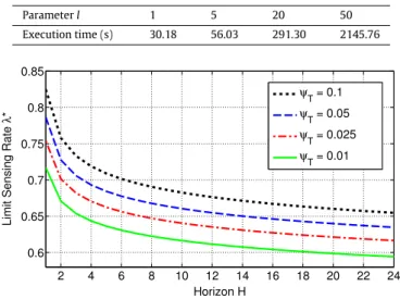
Execution time (s) 30.18 56.03 291.30 2145.76
Fig. 8. The limit sensing rateλ*as a function of the horizon H for four different values ofψ
T.
0.025, 0.05 and 0.1. We observe that
λ
*decreases as H increases. Moreover, as the outage probability constraint is relaxedand
ψ
Tis increased, higher sensing rates can be achieved while meeting the QoS constraint. For the threshold-based policies,one should make sure that
λ
min< λ
*so that the system is functional and the battery level remains positive throughout thespecified horizon for a given
ψ
T. Moreover,λ
maxmay be selected as large as the application requires in order to utilize theharvested energy.
4.4. Example III - State-Dependent Threshold Policy (SDTP)
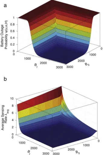
In this example, we set H
=
12,λ
min=
0.
4,λ
max=
10 and u=
3000, which means the battery is initially fully charged.We first show how
ψ
(u, α,
H) andλ
avg change as thresholds B0and B1vary between[
0,
3000]
inFig. 9from which onecan obtain the values of B0and B1that maximize
λ
avg while satisfyingψ
(u, α,
H)< ψ
Tfor a givenψ
T. We denote theseparticular values by B*0and B*1.
We also provide the execution time required to obtain the dataset ofFig. 9with a granularity of 50 for the threshold parameters B0and B1inTable 2. Obtaining the dataset ofFig. 9requires 612
=
3721 MRMFQ problem instances to solve.Also, recall thatFig. 9uses l
=
50 Erlangization levels only but the execution times inTable 2are obtained for varying values of the Erlangization parameter l. The average execution time per problem instance is less than a second even for the choice of a large Erlangization parameter, i.e., l=
50, but it can considerably be reduced to less than one tenth of a second with reduced l without sacrificing much from accuracy.InFig. 10, we demonstrate how the optimum thresholds B*
0and B*1behave as a function of H when
ψ
T=
0.
1, along withB*, the optimum threshold for the single threshold policy STP. For all values of H, B*appears to lie between B*
0and B*1but
for this example, all optimum thresholds appear to be close. For the same example, the average sensing rates
λ
avg obtainedby SDTP, and STP, and the limit sensing rate
λ
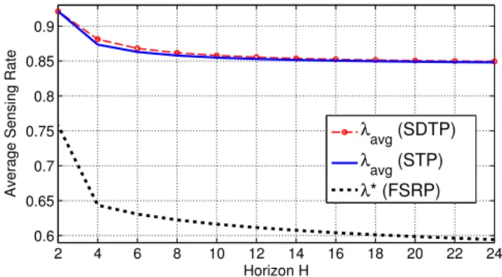
*is depicted inFig. 11as a function of the horizon parameter H. We observethat adaptive sensing increases substantially the average sensing rate if the adaptation is performed optimally. Moreover, the average sensing rate obtained by SDTP is slightly better than that of STP.
Fig. 9. (a) Battery outage probabilityψ(u, α,H) and (b) average sensing rateλavgas functions of B0and B1for u=3000, H=12,λmin=0.4 andλmax=10.
Fig. 10. Optimum thresholds B*
0, B*1, and B*as functions of the horizon H forψT=0.1, u=3000,α = [5/6 1/6],λmin=0.4 andλmax=10.
We now consider a 100-times slower EHP whose transition rates out of harvester states 1 and 0 are 1/500 and 1/100, respectively. For the following scenario, we set
α = [
1 0]
, which means that the initial harvester state is always 0. We also set
λ
min=
0.
9λ
*for all values of H. The other parameters are the same as in the previous scenario. We again plot theoptimum thresholds and average sensing rates inFigs. 12and13, respectively. B*still lies between B*
0and B*1which are quite
apart from each other. Moreover, STP is substantially outperformed by SDTP in terms of the average sensing rate. Similar to the relatively faster EHP, both SDTP and STP outperform FSRP for this example as well.
Fig. 11. Average sensing ratesλavgand limit sensing rateλ*as functions of the horizon H forψT =0.1, u=3000,α = [5/6 1/6],λmin =0.4 and
λmax=10.
Fig. 12. Optimum thresholds B*
0, B*1, and B*for 100-times slower process as functions of the horizon H forψT=,0.1, u=3000,α = [1 0],λmin=0.9λ*
andλmax=10.
Fig. 13. Average sensing ratesλavgand limit sensing rateλ*for 100-times slower process as functions of the horizon H forψT=0.1, u=3000,α = [1 0],
λmin=0.9λ*andλmax=10.
5. Conclusions
We propose in this paper a risk-theoretic multi-regime Markov fluid queue based method for computing finite-horizon battery outage probabilities in energy harvesting IoT devices. Subsequently, we use this method as the engine of an optimization framework by which we determine the optimum operational parameters of a so-called State-Dependent Threshold Policy (SDTP) which maximizes the average sensing rate while satisfying finite-horizon battery outage probability constraints. SDTP is compared and contrasted with numerical examples against other policies such as Fixed Sensing Rate Policy (FSRP) and Single Threshold Policy (STP). Threshold-based policies, namely SDTP and STP, outperform FSRP in terms of the average sensing rate in all the numerical examples we tried. We have also shown merit in using SDTP against STP for relatively slower EHPs. Future work will consist of more sophisticated models where sensing and packet transmission may
be uncoupled leading to two queues; one queue for energy and the other for data. Another future work will be related to obtaining optimum sensing rate policies that are more general than the double-valued policies extensively studied in this work.
Acknowledgment
The authors would like to thank the Science and Research Council of Turkey (TUBITAK) for supporting this study under project grant EEEAG-115E360.
References
[1] I. Akyildiz, W. Su, Y. Sankarasubramaniam, E. Cayirci, A survey on sensor networks, IEEE Commun. Mag. 40 (8) (2002) 102–114.
[2] J. Yick, B. Mukherjee, D. Ghosal, Wireless sensor network survey, Comput. Netw. 52 (12) (2008) 2292–2330.
[3] T. Arampatzis, J. Lygeros, S. Manesis, A survey of applications of wireless sensors and wireless sensor networks, in: Intelligent Control, 2005 Proceedings of the 2005 IEEE International Symposium on, Mediterranean Conference on Control and Automation, 2005, pp. 719–724.
[4] Y. Chen, Q. Zhao, On the lifetime of wireless sensor networks, IEEE Commun. Lett. 9 (11) (2005) 976–978.
[5] Ingenu, How RPMA Works:The Making of RPMA, Ebook by Ingenu, 2016.
[6] M. Centenaro, L. Vangelista, A. Zanella, M. Zorzi, Long-range communications in unlicensed bands: the rising stars in the IoT and smart city scenarios, IEEE Wirel. Commun. 23 (5) (2016) 60–67.
[7] K. Mikhaylov, J. Petaejaejaervi, T. Haenninen, Analysis of capacity and scalability of the LoRa low power wide area network technology, in: European Wireless 2016; 22th European Wireless Conference, 2016, pp. 119–124.
[8] G. Margelis, R. Piechocki, D. Kaleshi, P. Thomas, Low Throughput Networks for the IoT: Lessons learned from industrial implementations, in: Internet of Things (WF-IoT), 2015 IEEE 2nd World Forum on, 2015, pp. 181–186.
[9] S. Soro, W. Heinzelman, Prolonging the lifetime of wireless sensor networks via unequal clustering, in: Parallel and Distributed Processing Symposium, 2005 Proceedings. 19th IEEE International, 2005, pp. 236–244.
[10] N. Kaur, S.K. Sood, An energy-efficient architecture for the Internet of Things (IoT), IEEE Syst. J. (2015) in press.
[11] F.K. Shaikh, S. Zeadally, E. Exposito, Enabling technologies for green Internet of Things, IEEE Syst. J. (2015) in press.
[12] R. Vullers, R. Schaijk, H. Visser, J. Penders, C. Hoof, Energy harvesting for autonomous wireless sensor networks, IEEE Solid-State Circuit Mag. 2 (2) (2010) 29–38.
[13] S. Sudevalayam, P. Kulkarni, Energy harvesting sensor nodes: Survey and implications, IEEE Commun. Surv. Tutor. 13 (3) (2011) 443–461.
[14] M. Gorlatova, J. Sarik, G. Grebla, M. Cong, I. Kymissis, G. Zussman, Movers and shakers: Kinetic energy harvesting for the Internet of Things, in: The 2014 ACM International Conference on Measurement and Modeling of Computer Systems, SIGMETRICS ’14, ACM, New York, NY, USA, 2014, pp. 407–419.
[15] N. Michelusi, K. Stamatiou, M. Zorzi, Transmission policies for energy harvesting sensors with time-correlated energy supply, IEEE Trans. Commun. 61 (7) (2013) 2988–3001.
[16] J. Geng, L. Lai, Non-bayesian quickest change detection with stochastic sample right constraints, IEEE Trans. Signal Process. 61 (20) (2013) 5090–5102.
[17] M. Mandjes, D. Mitra, W. Scheinhardt, Models of network access using feedback fluid queues, Queueing Syst. 44 (4) (2003) 2989–3002.
[18] H.E. Kankaya, N. Akar, Solving multi-regime feedback fluid queues, Stoch. Models 24 (3) (2008) 425–450.
[19] M.A. Yazici, N. Akar, The finite/infinite horizon ruin problem with multi-threshold premiums: a Markov fluid queue approach, Ann. Oper. Res. (2016) in press.
[20] G. Jones, P. Harrison, U. Harder, T. Field, Fluid queue models of battery life, in: Modeling, Analysis Simulation of Computer and Telecommunication Systems, MASCOTS, 2011 IEEE 19th International Symposium on, 2011, pp. 278–285.
[21] G.L. Jones, Modelling Bursty Flows with Fluid Queues (Ph.D. thesis), Department of Computing, Imperial College London, 2014.
[22] S. Ulukus, A. Yener, E. Erkip, O. Simeone, M. Zorzi, P. Grover, K. Huang, Energy harvesting wireless communications: A review of recent advances, IEEE J. Sel. Areas Commun. 33 (3) (2015) 360–381.
[23] J. Yang, S. Ulukus, Optimal packet scheduling in an energy harvesting communication system, IEEE Trans. Commun. 60 (1) (2012) 220–230.
[24] V. Sharma, U. Mukherji, V. Joseph, S. Gupta, Optimal energy management policies for energy harvesting sensor nodes, IEEE Trans. Wirel. Commun. 9 (4) (2010) 1326–1336.
[25] C.K. Ho, P.D. Khoa, P.C. Ming, Markovian models for harvested energy in wireless communications, in: Communication Systems, ICCS, 2010 IEEE International Conference on, 2010, pp. 311–315.
[26] M.L. Ku, Y. Chen, K. Liu, Data-driven stochastic models and policies for energy harvesting sensor communications, IEEE J. Sel. Areas Commun. 33 (8) (2015) 1505–1520.
[27] P. Lee, Z.A. Eu, M. Han, H. Tan, Empirical modeling of a solar-powered energy harvesting wireless sensor node for time-slotted operation, in: Wireless Communications and Networking Conference, WCNC, 2011 IEEE, 2011, pp. 179–184.
[28] J. Lei, R. Yates, L. Greenstein, A generic model for optimizing single-hop transmission policy of replenishable sensors, IEEE Trans. Wirel. Commun. 8 (2) (2009) 547–551.
[29] H. Kantz, D. Holstein, M. Ragwitz, N.K. Vitanov, Markov chain model for turbulent wind speed data, Physica A 342 (12) (2004) 315–321. Proceedings of the VIII Latin American Workshop on Nonlinear Phenomena.
[30] A. Biason, M. Zorzi, Transmission policies for an energy harvesting device with a data queue, in: Computing, Networking and Communications, ICNC, 2015 International Conference on, 2015, pp. 189–195.
[31] N. Edalat, M. Motani, J. Walrand, L. Huang, A methodology for designing the control of energy harvesting sensor nodes, IEEE J. Sel. Areas Commun. 33 (3) (2015) 598–607.
[32] V. Joseph, V. Sharma, U. Mukherji, Optimal sleep-wake policies for an energy harvesting sensor node, in: Communications, 2009 ICC ’09 IEEE International Conference on, 2009, pp. 1–6.
[33] Y.M. Kadioglu, E. Gelenbe, Packet transmission with K energy packets in an energy harvesting sensor, in: Proceedings of the 2nd International Workshop on Energy-Aware Simulation, ENERGY-SIM ’16, ACM, New York, NY, USA, 2016, pp. 1:1–1:6.
[34] A. Kansal, J. Hsu, S. Zahedi, M.B. Srivastava, Power management in energy harvesting sensor networks, ACM Trans. Embed. Comput. Syst. 6 (4) (2007) 32.
[35] C. Vigorito, D. Ganesan, A. Barto, Adaptive control of duty cycling in energy-harvesting wireless sensor networks, in: Sensor, Mesh and Ad Hoc Communications and Networks, 2007 SECON ’07 4th Annual IEEE Communications Society Conference on, 2007, pp. 21–30.
[36] R. Chan, P. Zhang, W. Zhang, I. Nevat, A. Valera, H.-X. Tan, N. Gautam, Adaptive duty cycling in sensor networks via Continuous Time Markov Chain modelling, in: Communications ,ICC, 2015 IEEE International Conference on, 2015, pp. 6669–6674.