Mean-field theory for Bose-Hubbard model under a magnetic field
M. Ö. Oktel,1,*M. Niţă,2and B. Tanatar1
1Department of Physics, Bilkent University, 06800 Bilkent, Ankara, Turkey
2Institute of Physics and Technology of Materials, P.O. Box MG7, Bucharest-Magurele, Romania 共Received 25 April 2006; revised manuscript received 16 August 2006; published 31 January 2007兲 We consider the superfluid-insulator transition for cold bosons under an effective magnetic field. We inves-tigate how the applied magnetic field affects the Mott transition within mean-field theory and find that the critical hopping strength共t/U兲cincreases with the applied field. The increase in the critical hopping follows the bandwidth of the Hofstadter butterfly at the given value of the magnetic field. We also calculate the magneti-zation and superfluid density within mean-field theory.
DOI:10.1103/PhysRevB.75.045133 PACS number共s兲: 67.40.Db, 05.30.Jp, 05.70.Fh
I. INTRODUCTION
One of the most interesting developments in ultracold atom physics is the study of neutral atoms in optical lattices.1
An optical lattice is prepared by creating a periodic potential utilizing a standing wave of light, and optical lattices in one, two, and three dimensions have been realized experimen-tally.
The cooling, trapping, and coherent manipulation of the atomic motion by their interaction with light has been estab-lished by numerous investigations in the field of atom interferometers,2 matter-wave superradiance,3 matter-wave
parametric amplifiers,4,5 and others.6 One should mention
also the opportunities garnered by using the ultracold alkali atoms as quantum computers,7or by using the Mott
insulat-ing state of neutral bosonic atoms for detection of quantum entanglement.8–10The custom-made trapping potentials in the
optical lattice has also opened a venue to study many con-densed matter problems, such as the Mott insulator transition experimentally realized by Greiner et al.11
Although many different regimes exist for optical lattice experiments, one that is quite interesting from a theoretical point of view is that of a deep lattice with few particles per lattice site. If fermions are used instead of bosons, these ex-periments may lead to direct realization of many correlated electron model Hamiltonians such as the Hubbard model of high-temperature superconductivity or lattice Quantum Hall models.12
In this work, we concentrate on bosons, and assume that at each lattice site there is only one available state共that is equivalent to requiring the first excited state at each lattice site to be sufficiently high in energy兲. In this case the Hamil-tonian is13 H = − t
兺
具ij典共ai † aj+ aj † ai兲 + U 2兺
i 共ni− 1兲ni−兺
i ni, 共1兲where aiis the annihilation operator at site i and ni= ai†ai is
the number operator at site i. The first term corresponds to hopping between different lattice sites and for practical pur-poses only nearest-neighbor hopping is important, so the sum 具ij典 is carried over the nearest neighbors. The second term is the particle-particle interaction and the last term is the chemical potential. This is the widely studied Bose-Hubbard Hamiltonian.13–15
The strong tunneling limit between optical lattice sites 共U/tⰆ1兲 corresponds to the superfluid 共SF兲 phase. Changing the laser intensity with increasing depth of the optical poten-tial the atomic waves become more localized and the on-site interaction U increases at the same time with the reduction of the tunneling parameter t.15 The system is driven to a Mott
insulator 共MI兲 phase and loses long-range phase coherence. In general, if the interaction is strong enough the system prefers a particle number that is commensurate with the number of lattice sites and the system goes into the insulat-ing phase. The strength of interaction U needed for this tran-sition is roughly the bandwidth of the noninteracting system 2zt, where z is the number of nearest neighbors.
A much less studied problem is that of the Bose-Hubbard Hamiltonian under a magnetic field. Experimentally, of course, the bosons used in cold gas experiments are un-charged and would not be directly affected by an external magnetic field. However, recent studies have shown in detail how a magnetic Hamiltonian, or, in general, effective elec-tromagnetic fields, can be generated for atoms in optical lat-tices using an external time varying electric field16 by an
oscillating quadrupole potential together with a periodic modulation of the tunneling between lattice sites17 or using more complicated laser configurations.18 These
investiga-tions suggest that it may be possible to study such systems with reasonable improvements on already functioning ex-periments. An effective magnetic field can also be created by rotating the optical lattice, and cancelling the centrifugal force of the rotation by an external quadratic trap.19We also
note the two recent papers which study how the artificial external non-Abelian gauge potentials can be created for cold atom systems.20,21
In this work, we assume that we have a two-dimensional square lattice in the x-y plane, under a magnetic field in the z direction. We also consider that the “charged bosons” are interacting only when they are on the same lattice site and the temperature of the system is set to zero. In this case the Hamiltonian is H = − t
兺
n,m 关anm † a共n+1兲m+ ei2nanm † an共m+1兲+ H.c.兴 共2兲 +U 2兺
n,m共anm † a nm− 1兲anm† anm−兺
n,m anm† anm. 共3兲Here, we label every site of the lattice i , j by two integers i =共ni, mi兲=共n,m兲, one integer 共n兲 along the x axis, the other
共m兲 along the y axis, and choose the gauge to be Aជ= xyˆ. The first term is the usual hopping term, where hopping along the y axis gets a phase shift due to the presence of the magnetic field. Magnetic field affects the system through the parameter
with
= Bl2/
0, 共4兲
where l is the lattice spacing and 0 is the flux quantum. Thus, the parameter measures the magnetic flux per unit cell of the lattice in units of flux quantum. The second and third terms are interactions and chemical potential, respec-tively. Even at U = 0, the noninteracting limit of this Hamil-tonian shows interesting results; the energy spectrum at U = 0 is known as the Hofstadter butterfly.22 The most
impor-tant aspect of the noninteracting problem is that the band-width depends critically on, and gaps open up or close in a self-similar manner. With such a complicated single particle spectrum, it is not at all clear how the presence of the mag-netic field will change the Mott transition, or whether more exotic phases can be found.
We believe that with the possibility of experimental real-ization, it is of importance to study this model more closely and understand its rich phase diagram. In this work, we con-centrate on the superfluid-insulator transition and investigate the effect of the external magnetic field on the phase bound-ary. Our mean-field approach is not capable of capturing pos-sible correlated phases, however it may serve as a basis for more detailed investigation of the model.
We find that the Mott insulating phases become more stable under the applied magnetic field, an expected effect as one of the most important effects of the magnetic field would be to localize particles further. More importantly, we find that the critical hopping to interaction ratio t / U roughly fol-lows the bandwidth of the Hofstadter butterfly. We also cal-culate the magnetization and the superfluid density within mean-field theory.
In the rest of this paper we first outline our calculational scheme of solving the Bose-Hubbard model under a mag-netic field within the mean-field approach. We then present our results on the phase diagram identifying the superfluid and insulating regions. We conclude with a brief summary of our main results.
II. MEAN-FIELD APPROACH
Our calculations are based on the mean-field approach of the Bose-Hubbard Hamiltonian,23by considering the
follow-ing decouplfollow-ing formula for the product of the two Bose field operators:
anm† a共n+1兲m=具anm† 典a共n+1兲m+ anm† 具a共n+1兲m典 − 具anm† 典具a共n+1兲m典.
共5兲 The average value具anm† 典 represents the order parameter ⌿nm
that accounts for the insulator-superfluid transition. It is equal to zero on the insulator side of the transition when the ground state of the system has a definite particle number on
every site of the lattice, and has a nonzero value for the superfluid state when there are large quantum fluctuations of the atom number in the optical lattice. In this case 兩⌿nm兩2
represents the local density of the atoms in the condensate state.
Using Eq.共5兲 the Bose-Hubbard Hamiltonian given in Eq.
共2兲 turns into a sum of the following single-site terms:
Hnm MF= − t关⌿ 共n+1兲m * a nm † +⌿ 共n−1兲m * a nm † + ei2n⌿ n共m+1兲 * a nm † + e−i2n⌿n*共m−1兲anm† + H.c.兴 + U共nnm− 1兲nnm−nnm + Cnm, 共6兲
where nnmis the single-site density operator anm† anmand Cnm
is a constant energy term.
The matrix elements of the mean-field HamiltonianHnm MF
in the occupation number base兩Nnm典 are given by
具Nnm兩Hnm MF兩N nm典 = 1 2UNnm共Nnm− 1兲 −Nnm+ Cnm, 共7兲 具Nnm+ 1兩Hnm MF兩N nm典 = − t
冑
Nnm+ 1关⌿共n+1兲m* +⌿共n−1兲m* + ei2n⌿ n共m+1兲 * + e−i2n⌿ n共m−1兲 * 兴, 共8兲 where we used the property of the Bose field operators c兩N + 1典=冑
N + 1兩N典 and c†兩N典=冑
N + 1兩N+1典. All other matrix el-ements are zero, except the conjugate elel-ements of Eq. 共8兲.We note that the occupation number Nnmabove varies from 0
to ⬁ and they are referred to the site 共nm兲 of the optical lattice. We diagonalize the Hamiltonian equation 共6兲 in a
truncated basis 兩Nnm典 with Nnm= 0 . . . Nmax and calculate the
ground state of the mean-field Hamiltonian,
兩Gnm典 =
兺
N=0 Nmax ␣N nm兩N nm典, 共9兲with the coefficients␣N nm
corresponding to the lowest eigen-value of the matrix of Eq.共6兲 in the truncated base.
The order parameter corresponding to the ground state given by Eq.共9兲 will be
⌿nm=具Gnm兩anm † 兩Gnm典 =
兺
N=0 Nmax−1 ␣N nm*␣ N+1 nm冑
N + 1. 共10兲 For a given truncated basis the equations of the finite Hermitian matrix in Eq.共7兲 and Eq. 共8兲 and the formula forthe SF order parameter, Eq. 共10兲, represent a set of
self-consistent equations that give the solution of the ground state of the single site Hamiltonian, Eq.共6兲, and the order
param-eters⌿nmin the mean-field approximation.
The numerical calculations are repeated with increasing values of the dimension Nmax of the truncated basis to attain
convergence of the solution. In the mean-field approxima-tion, the ground state of the Bose-Hubbard Hamiltonian, Eq. 共2兲, is given by the direct product of the single site ground
states of Eq.共9兲,
兩G典 =
兿
nm
For a given ground state, Eq.共9兲, the probability for the
single site operator nnmto take the value N will be given by
the square of the corresponding developing coefficient␣N nm
. The average single site occupation number denoted with
共nm兲 is equal to 共nm兲 = 具nnm典 =
兺
N=1 Nmax 兩␣N nm兩2N, 共12兲and the condensate component of the superfluid density, within mean-field theory, on the site nm is
s共nm兲 = 兩⌿nm兩2. 共13兲
We denote by andsthe surface average of 共nm兲 and
s共nm兲, respectively. For a noninteracting system at zero
temperature all of the bosons are in the condensate, i.e., in the lowest single particle state of the lattice, and we have =s. When the interaction increases关nonzero values of U in
Eq. 共2兲兴 only a significant fraction of the bosons will
con-dense in the same single particle quantum state, and we have
s⬍. The competition between the kinetic energy of the
system t and interaction U gives rise to interesting successive transitions between a superfluid and a Mott insulator.
The mean-field solution of the nonmagnetic system and the phase diagram are calculated by Sheshadri et al.23 See
also the Mott insulator lobes in Figs.1 and2. For the mag-netic Hamiltonian, perturbative techniques are used by Ni-emeyer et al.,24where the MI lobes are calculated for small
values of the magnetic flux= 0 , . . . , 0.125.
Introducing the magnetic field in the hopping term of the Hamiltonian of Eq.共2兲 breaks the temporal invariance of the
Hamiltonian and gives rise to persistent current flow of the “charged bosons.” For any bond connecting neighboring sites共i;k兲=共n,m;n±1,m兲 关or 共i;k兲=共n,m;n,m±1兲兴 of the lattice, we define tik= t for hopping along x共or tik= tei2nfor
hopping along y兲. We calculate the local bond current of the superfluid phase using the following formula:
vik= 1 iប关tikai † ak− tkiak † ai兴, 共14兲 by substituting 具ai † ak典 with 具⌿i⌿k *典. Another parameter of interest is the magnetic momentum. In the mean-field decou-pling we can define the single site magnetization by the fol-lowing formula: Mnm= n¯vx共nm兲 − mv¯y共nm兲 = − 1 ប d⍀nm d , 共15兲 where ⍀nm is the average value of the mean-field
Hamil-tonian of Eq. 共6兲 with respect to the ground state, Eq. 共9兲,
and represents the single site energy of the Bose gas. The averaged site velocities¯vx,y共nm兲 are equal to the average of
the bond currents of Eq.共14兲 connecting the site n,m to its
neighbors along x or y accordingly. The magnetic momen-tum denoted with M is equal to the surface average of Eq.共15兲.
For zero magnetic field the two-dimensional共2D兲 lattice has the translational invariance along both axes and the order parameter⌿nmdoes not depend on the site index共nm兲.
In our case, for nonzero magnetic field in the chosen Lan-dau gauge the system preserves only the invariance along the y axis of the lattice. Therefore, the order parameter is chosen as ⌿nm=⌿n. In this case, we calculate the mean-field
solu-tion for a given ratio of the magnetic flux= p / q. From the equation of the matrix elements of the mean-field equation 共8兲, it can be noted that the periodicity of the solution is
⌿n=⌿n+q. The same periodicity condition is verified by the
the density that also shows the translational invariance along the y axis: 共nm兲=共n兲 and 共n兲=共n+q兲. To solve the mean-field equations we choose a finite sequence of the lattice of dimension q in x direction and impose periodic boundary conditions. In the Landau gauge, the system is pe-riodic with lattice pepe-riodicity in the y direction, thus our calculations are carried out on a 1⫻q supercell with periodic boundary conditions. We measure the energy in units of U 共i.e., U=1兲.
III. RESULTS AND DISCUSSION
Based on our calculations outlined in the preceding sec-tion, we now present our numerical results. The two possible states of the 2D Bose system are selected as follows: in the MI phase, the on-site occupation number has integer values and the variance of is zero; in the SF phase the on-site occupation number has noninteger values and the variance
共兲⫽0. The main features of our results are illustrated in Figs.1–6.
The phase diagram in the, t plane is depicted in Fig.1, which is calculated for= 0 and= 0.1. For the Mott insu-lator state the site occupation number共nm兲 is equal toand has integer values 共see Mott lobes in Fig. 1 for = 1 , 2 , 3兲. The variance of is equal to zero for the MI state and has large fluctuations for the SF state 共see the variance of in Fig.2兲.
The Bose-Hubbard model under a magnetic field has also been considered by Niemeyer, Freericks, and Monien,24
us-ing strong couplus-ing expansion. Strong couplus-ing expansion utilizes a perturbative expansion in t / U, and is valid within the Mott insulating regime for small t / U and small values of the flux . The mean-field approach of this paper, on the other hand, is a self-consistent but uncontrolled approxima-tion, which makes it possible to calculate physical quantities for both the insulating and the superfluid regimes. Although the two approximation methods have very different charac-ter, they generally yield qualitatively similar results. Very similar phase diagrams have been obtained by these two dif-ferent approaches for the pure Bose-Hubbard model 共Refs.
23and25兲, and the superlattice Bose-Hubbard model 共Refs. 26 and 27兲. Indeed, we find that our mean-field treatment
produces a qualitatively similar result to the strong coupling expansion for the Bose-Hubbard model under a magnetic field. However, our method allows us to extend the calcula-tion to the full range of magnetic flux 0⬍⬍1, and calcu-late the superfluid density and magnetization in the super-fluid phase.
We note that the transition point at zero magnetic flux is located at tc= 0.043 for= 0.5共c.f. Fig.1兲. This corresponds
to U / 4t = 5.8 which is equal to the transition point deter-mined by van Oosten et al.28
The magnetic flux breaks the temporal invariance of the system and destroys the coherence of the wave function in a 2D fermion system after a “flight” time proportional29 to
1 / B. For a Bose system, the magnetic flux can have the same effect over the SF coherent wave function, destroying the stability of the superfluid solution in the proximity of the transition point and leading to the SF-MI transition when is bigger than a critical valuec. This is consistent with the
increased area of the Mott lobes when the magnetic field is present as shown in Figs. 1 and 2. For all values of the magnetic flux we depicted the phase diagram in the t ,plane for the different values of the chemical potential in Fig.3.
We note the above MI-SF transition for a constant t value, increasing the magnetic fluxfrom zero to the critical tran-sition pointc. For smallthe optical lattice approximates a
continuous system of charged bosons under the magnetic field and the superfluid-insulator transition is similar to the disappearance of the superconductivity when the external magnetic flux in a superconductor exceeds a critical value.30
However, for the Bose-Hubbard Hamiltonian the discrete-ness of the lattice brings about other interesting features. The noninteracting spectrum22 is periodic in with ⌬= 1 and symmetric around the value = 0.5. We recover the same feature of the phase diagram in Fig.3.
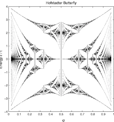
One of the most important results of our calculation is displayed in Fig. 3. The oscillations of the critical hopping strength with changing magnetic field follow the oscillations of the bandwidth of the Hofstadter butterfly22 共see Fig. 4兲.
For instance, increasing causes the bandwidth of the
Hof-stadter butterfly system22 to shrink, meaning that the
super-fluid order appears at a smaller value of U共or higher value of t兲. For →0.5 the bandwidth of the Hofstadter butterfly is increased again and the critical value tc of the transition is
increased. This suggests that in the phase diagram of Fig.3
共calculated for U=1兲, the critical point 共U/t兲cof the SF-MI
transition is proportional to the bandwidth of the Hofstadter butterfly.22
The loss of translational invariance of the charged bosons under a magnetic field is correlated with the appearance of the surface oscillations of the particle density in the super-fluid phase. Although one expects a spontaneous breaking of the translational invariance in the superfluid phase, such as vortex states, in our mean-field approach this symmetry is explicitly broken by our gauge choice. Physically measur-able quantities should be independent of the choice of the gauge, however our mean-field treatment yields spatially de-pendent parameters such as 兩⌿n兩2, which depend on the
gauge choice. Still, it is not unreasonable to expect that spa-tially averaged quantities such assand magnetization to be
correctly captured by our approach. For certain values of the magnetic field we verified this expectation by using the sym-metric gauge and corresponding square supercell. Also, as the insulator side of the transition is spatially uniform, ex-plicit determination of the gauge should not strongly affect the MI-superfluid phase boundaries. In Fig. 5 we show the variance of the on-site SF order parameter⌿nwhen the
hop-ping parameter t is increased, for different points of the lat-tice n. Even all the SF order parameters⌿nexhibit the
dis-appearance of the insulator order at the same critical value, FIG. 1.共Color online兲 Phase diagram of Bose atoms confined in
a 2D optical lattice for the magnetic flux=0 共left panel兲 and 0.1 共right panel兲. In the figure the first three Mott lobes are depicted, for on-site particle numbers 1, 2, and 3.
FIG. 2. 共Color online兲 Phase diagram for the magnetic flux = 0共right panel兲 and 0.4 共left panel兲. On the z axis the variance共兲 of the Bose density is plotted. For the MI phase the variance of the 2D density is zero, and the Bose charge has no fluctuation.
t = tc, the rate of increase of ⌿n for t⬎tc is different for
different points of the lattice. There are points in the lattice that show a very low rate of increase of ⌿n. The figure
clearly shows the surface oscillations of the “charge” density in the optical lattice. It means that, for t⬎tc, there are
re-gions in the lattice with small SF order parameter and small density fluctuations. It is possible to interpret these as the superfluid density oscillations due to the presence of vorti-ces. However, close to the Mott transition where these gions are most pronounced, correlations between such re-gions may develop, causing a phase transition which would not be captured by our mean-field treatment.
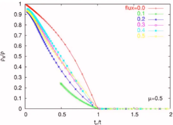
The lower rate of increase of the superfluid order param-eter vs t, for t⬎tc, is also suggested in the scaled curves in
Fig.6 that show the ratio/s versus tc/ t. For tc/ tⱗ1, the
SF phase is strongly affected by the magnetic field presence, and we note the change of the curve slope in Fig.6 for ⫽0. For tc/ t→0, the magnetic field has no effect, and all
Bose particles tend to condense共/s→1 for allvalues in
Fig.6兲. We also notice that even a small magnetic field
= 0.1 affects the superfluid density rather strongly. For such small magnetic fields our approach is less reliable, as the cell size used in our calculations is inversely proportional to the flux. While similar discontinuous effects at zero field have
been discussed within the context of Josephson junction arrays,31we cannot clarify the behavior near zero field due to
the limitations of our numerical mean-field approach. Figure 7 shows the magnetization as a function of the hopping parameter t for different values of the magnetic flux
= 0.1, 0.2, 0.3, and 0.4 at the chemical potential= 0.5. We note that our approach is less reliable for the case of = 0.1, as the number of particles per site increase most quickly in this case. For t⬍tc, in the MI phase, the
magne-tization is equal to zero and the particle motion is frozen. For t⬎tc, in the SF phase, the curves exhibit negative values of
magnetization, meaning the existence of persistent current flow. We note that the sign of the magnetization is related to the slope of the energy curve vs magnetic flux in Hofstadter butterfly.32
The change of slope of the eigenstates as a function of in the Hofstadter butterfly gives rise to changes in the sign of the magnetization near the special values of the magnetic flux共for instance= 1 / q; see Ref.22兲. We do not expect this
fine effect to be observable in the lowlimit. In this case, the small fluctuations of thefor the real system gives rise to the smeared graph of the spectrum.22
For苸关0.45,0.5兴 the magnetization can have an oppo-site sign共compared with the values for苸关0,0.45兴兲 as the slope of the Hofstadter spectrum vs clearly changes 共see Ref.22or Fig.3兲.
IV. SUMMARY
We calculated the mean-field phase diagram of the 2D Bose-Hubbard Hamiltonian under a perpendicular magnetic FIG. 3.共Color online兲 Phase diagram of Bose atoms confined in
a 2D optical lattice in the t- plane for different values of the chemical potential, corresponding to the MI phase with=1 共top兲 and=2 共bottom兲. The curves correspond to the critical values tcof the SF-MI transition. For t⬎tcthe system is in the superfluid phase and for t⬍tcin the MI phase. The phase diagram is periodic in the magnetic flux with⌬=1 and symmetric around the flux value = 0.5.
FIG. 4. Single particle energy bands as a function of magnetic flux per plaquette, the Hofstadter butterfly共Ref.22兲.
field. The Mott insulator-superfluid transition is strongly af-fected, and the features around the transition point resemble the interesting property of the Hofstadter butterfly. The en-ergy spectrum for the noninteracting case exhibits periodicity with ⌬= 1, symmetry around the value = integer/ 2 and striking oscillations22 that lead to similar features of the
MI-SF transition when the magnetic field is varied共see the phase diagram in the t ,plane in Fig.3兲.
In the superfluid phase, at zero magnetic field the system has time translational invariance and the net local current of the Bose particles is zero because the reversed Bose paths are equally probable. Even for a small value of the time in-variance is suddenly broken and the reversal paths of the coherent Bose atoms are not equally probable anymore共in fact only one of the two reversal paths is permitted; the other one corresponds to change of the sign of the magnetic flux兲. The persistent currents of the Bose particles appear, leading to a nonzero value of the orbital magnetization. We note also the surface charge oscillations that are not present in the SF phase with translational invariance when the magnetic field is set to zero.
The surface charge oscillations are not present for the MI phase. At low values of the SF phase exhibit negative susceptibility when the magnetic field is applied and at a critical value the system is driven into the insulating phase. This is the continuous limit of the model and the behavior of the Bose system shows features resembling that of the Meissner effect in superconductors. For higher kinetic en-ergy共large values of t/U兲 this scenario is not valid anymore, the magnetic flux loses its effect over the quantum state of the Bose system and the system preserves its SF character-istics, albeit with spatial oscillations of its order paremeter. We hope our work stimulates further experimental and theo-retical interest in this model.
FIG. 5. 共Color online兲 SF order parameter ⌿nfor different lat-tice sites at MI-SF transition. The chemical potential is=0.5 cor-responding to MI with=1 and=1.5 corresponding to MI with =2. The blue line with crosses represents the surface average value⌿. For t⬎tcthe second derivative d2⌿/dt2changes sign for the points n = 4 , 5. The magnetic flux is=0.1 and the superfluid order parameter has the periodicity⌿n=⌿n+10. For the SF phase共at
t⬎tc兲 the lattice sites integer⫻10+4 and integer⫻10+5 exhibit
very low values of the SF order parameter and low variance of.
FIG. 6. 共Color online兲 s/ as a function of tc/ t for different values of the magnetic flux. For=0 our curve is similar to Fig. 1 of Ref.23. The change of slope at t⯝ ⬎tcfor⫽0 is related to the surface oscillations of the charged bosons. When the magnetic field is present, the superfluid phase exhibits surface region where the quantum fluctuations of SF density and the order parameter are small 共compared to nearby regions; see Fig.5兲 meaning that the
local phase is closer to an insulator. It exhibits a lower ratios/ compared with the case=0.
FIG. 7. 共Color online兲 Magnetization as a function of t for = 0.1, 0.2, 0.3, 0.4共from top to bottom兲. In the MI phase, for t⬍tc, the magnetization is zero. Our numerical approach is more reliable at lower values of t, and not too small, where our computational supercell size is small and the number fluctuations at each lattice site are limited. MI and superfluid phases and tc are identified for =0.1 on the figure. The value of tcfor other can be identified as the point where magnetization becomes nonzero on the correspond-ing curve.
ACKNOWLEDGMENTS
M. N. acknowledges the support from TUBITAK and CERES and thanks the Department of Physics, Bilkent
Uni-versity for hospitality during the time part of this work was performed. M.Ö.O is supported by TUBA-GEBIP Grant and TUBITAK-Kariyer Grant No. 104T165. B.T. gratefully ac-knowledges partial support from TUBITAK and TUBA.
*Electronic address: [email protected]
1G. Raithel, G. Birkl, A. Kastberg, W. D. Phillips, and S. L. Rolston, Phys. Rev. Lett. 78, 630共1997兲; S. E. Hamann, D. L. Haycock, G. Klose, P. H. Pax, I. H. Deutsch, and P. S. Jessen,
ibid. 80, 4149共1998兲; L. Guidoni, C. Triché, P. Verkerk, and G.
Grynberg, ibid. 79, 3363共1997兲; M. Raizen, C. Salomon, and Q. Niu, Phys. Today 50共7兲, 30 共1997兲.
2F. Burgbacher and J. Audretsch, Phys. Rev. A 60, R3385共1999兲. 3S. Inouye, A. P. Chikkatur, D. M. Stamper-Kurn, J. Stenger, D. E.
Pritchard, and W. Ketterle, Science 285, 571共1999兲.
4M. Kozuma, Y. Suzuki, Y. Torii, T. Sugiura, T. Kuga, E. W. Hagley, and L. Deng, Science 286, 2309共1999兲.
5S. Inouye, T. Pfau, S. Gupta, A. P. Chikkatur, A. Görlit, D. E. Pritchard, and W. Ketterle, Nature共London兲 402, 641 共1999兲. 6For a collection of review articles, see the special issue of Nature
共London兲 416, 206 共2002兲.
7E. Jane, G. Vidal, W. Dur, P. Zoller, and J. I. Cirac, Quantum Inf. Comput. 3, 15共2003兲.
8O. Mandel, M. Greiner, A. Widera, T. Rom, T. W. Hänsch, and I. Bloch, Nature共London兲 425, 937 共2003兲.
9W. K. Hensinger, H. Häffner, A. Browaeys, N. R. Heckenberg, K. Helmerson, C. McKenzie, G. J. Milburn, W. D. Phillips, S. L. Rolston, H. Rubinsztein-Dunlop, and B. Upcroft, Nature 共Lon-don兲 412, 52 共2001兲.
10C. M. Alves and D. Jaksch, Phys. Rev. Lett. 93, 110501共2004兲. 11M. Greiner, O. Mandel, T. Esslinger, T. W. Hänsch, and I. Bloch, Nature共London兲 415, 39 共2002兲; M. Greiner, O. Mandel, T. W. Hänsch and I. Bloch, ibid. 419, 51共2002兲.
12B. Paredes, P. Zoller, and J. I. Cirac, Phys. Rev. A 66, 033609 共2002兲; N. Regnault and Th. Jolicoeur, Phys. Rev. Lett. 91, 030402共2003兲.
13See for a recent review, D. Jaksch and P. Zoller, Ann. Phys. 315, 52共2005兲.
14M. P. A. Fisher, P. B. Weichman, G. Grinstein, and D. S. Fisher, Phys. Rev. B 40, 546共1998兲.
15D. Jaksch, C. Bruder, J. I. Cirac, C. W. Gardiner, and P. Zoller, Phys. Rev. Lett. 81, 3108共1998兲, and references therein. 16D. Jaksch and P. Zoller, New J. Phys. 5, 56共2003兲.
17A. S. Sorensen, E. Demler, and M. D. Lukin, Phys. Rev. Lett. 94, 086803共2005兲.
18E. J. Mueller, Phys. Rev. A 70, 041603共R兲 共2004兲.
19S. Tung, V. Schweikhard, and E. A. Cornell, Phys. Rev. Lett. 97, 240402共2006兲.
20K. Osterloh, M. Baig, L. Santos, P. Zoller, and M. Lewenstein, Phys. Rev. Lett. 95, 010403共2005兲.
21J. Ruseckas, G. Juzeliunas, P. Ohberg, and M. Fleischhauer, Phys. Rev. Lett. 95, 010404共2005兲.
22D. R. Hofstadter, Phys. Rev. B 14, 2239共1976兲.
23K. Sheshadri, H. R. Krishnamurthy, R. Pandit, and T. V. Ramakrishnan, Europhys. Lett. 22, 257共1993兲.
24M. Niemeyer, J. K. Freericks, and H. Monien, Phys. Rev. B 60, 2357共1999兲.
25J. K. Freericks, and H. Monien, Phys. Rev. B 53, 2691共1996兲. 26P. Buonsante and A. Vezzani, Phys. Rev. A 70, 033608共2004兲. 27P. Buonsante and A. Vezzani, Phys. Rev. A 72, 013614共2005兲. 28D. van Oosten, P. van der Straten, and H. T. C. Stoof, Phys. Rev.
A 63, 053601共2003兲.
29G. Bergmann, Phys. Rep. 207, 1共1984兲.
30M. Tinkham, Superconductivity共McGraw-Hill, New York, 1996兲. 31Q. Niu and F. Nori, Phys. Rev. B 39, 2134共1989兲.