PERFORMANCE IMPROVEMENT ON
LATENCY-BOUND PARALLEL HPC
APPLICATIONS BY MESSAGE SHARING
BETWEEN PROCESSORS
a thesis submitted to
the graduate school of engineering and science
of bilkent university
in partial fulfillment of the requirements for
the degree of
master of science
in
computer engineering
By
Mustafa Duymu¸s
February 2021
Performance improvement on latency-bound parallel HPC applications by message sharing between processors
By Mustafa Duymu§
February 2021
vVe certify that we have read this thesis and that in our opinion it is fully adequate, in scope and in quality, as a thesis for the degree of Master of Science.
Can Alkan
•
MuratM�
Approved for the Graduate School of Engineering and Science:
Director of the Graduate School 11
ABSTRACT
PERFORMANCE IMPROVEMENT ON
LATENCY-BOUND PARALLEL HPC APPLICATIONS
BY MESSAGE SHARING BETWEEN PROCESSORS
Mustafa Duymu¸s
M.S. in Computer Engineering Advisor: Cevdet Aykanat
February 2021
The performance of paralellized High Performance Computing (HPC) applica-tions is tied to the efficiency of the underlying processor-to-processor commu-nication. In latency-bound applications, the performance runs into bottleneck by the processor that is sending the maximum number of messages to the other processors. To reduce the latency overhead, we propose a two-phase message-sharing-based algorithm, where the bottleneck processor (the processor sending the maximum number of messages) is paired with another processor. In the first phase, the bottleneck processor is paired with the processor that has the maxi-mum number of common outgoing messages. In the second phase, the bottleneck processor is paired with the processor that has the minimum number of outgo-ing messages. In both phases, the processor pair share the common outgooutgo-ing messages between them, reducing their total number of outgoing messages, but especially the number of outgoing messages of the bottleneck processor. We use Sparse Matrix-Vector Multiplication as the kernel application and a 512-processor setting for the experiments. The proposed message-sharing algorithm achieves a reduction of 84% in the number of messages sent by the bottleneck processor and a reduction of 60% in the total number of messages in the system.
Keywords: High Performance Computing, Parallel applications, MPI, Store-and-Forward Algorithms.
¨
OZET
GEC˙IK˙IM-L˙IM˙ITL˙I PARALEL UYGULAMALARDA
˙IS¸LEMC˙ILER ARASI MESAJ PAYLAS¸IM
Y ¨
ONTEM˙IYLE PERFORMANS ˙IY˙ILES
¸T˙IRME
Mustafa Duymu¸s
Bilgisayar M¨uhendisli˘gi, Y¨uksek Lisans Tez Danı¸smanı: Cevdet Aykanat
February 2021
Paralelle¸stirilmi¸s Y¨uksek Performanslı Hesaplama (HPC) uygulamalarının ba¸sarımı, arka plandaki i¸slemci-i¸slemci ileti¸siminin verimlili˘gine ba˘glıdır. Gecikim-darbo˘gazlı uygulamalarda performans, en fazla mesaj g¨onderen i¸slemci tarafından limitlenir. Gecikim ek y¨uk¨un¨u d¨u¸s¨urmek i¸cin en fazla mesaj g¨onderen i¸slemcinin ba¸ska bir i¸slemci ile e¸slendi˘gi iki-fazlı mesaj-payla¸sma-temelli bir algo-ritma ¨onermekteyiz. Birinci fazda, en fazla mesaj g¨onderen i¸slemci, sistemdeki di˘ger i¸slemciler i¸cerisinden en fazla ortak giden mesaja sahip oldu˘gu i¸slemci ile e¸slenir. ˙Ikinci fazda ise, en fazla mesaj g¨onderen i¸slemci, en az mesaj g¨onderen i¸slemci ile e¸slenir. Her iki fazda da e¸slenen i¸slemciler, ortak giden mesajları ar-alarında payla¸sarak mesaj sayılarını d¨u¸s¨urmektedir. Bu, ¨ozellikle de en fazla mesaj g¨onderen i¸slemcinin g¨onderdi˘gi mesaj sayısını d¨u¸s¨urmektedir. C¸ ekirdek i¸slem olarak seyrek matris-vekt¨or ¸carpımı kullanılmı¸s ve testler 512 i¸slemcili bir sistemde yapılmı¸stır. ¨Onerilen mesaj-payla¸sma-temelli algoritma en fazla mesaj g¨onderen i¸slemcinin g¨onderdi˘gi mesaj sayısında %84, sistemdeki toplam mesaj sayısında %60 d¨u¸s¨u¸se imkan tanımı¸stır.
Anahtar s¨ozc¨ukler : Y¨uksek Performanslı Hesaplama, Paralel Uygulamalar, MPI, Sakla-ve-y¨onlendir Algoritmaları.
Acknowledgement
Firstly, I would like to thank my supervisor Prof. Cevdet Aykanat for all his guidance. Since we met in CS473 course more than four years ago, he always in-spired and motivated me with a great understanding in every part of my academic career.
I also thank my jury members Asst.Prof. Can Alkan and Prof. Murat Man-guo˘glu for reading my thesis and providing constructive feedback.
I owe a special thanks to Dr. Ozan Karsavuran, who provided a great help for this work. Without his contribution, this work would not have been completed.
I also would like to thank my friends O˘guzhan, ˙Ilayda and Akifhan. Apart from all the beautiful moments we had in our offices and the campus, nearly-everyday talks and discussions we had helped to overcome the depressing solitude of quarantine life.
With a special place in my life and in my heart, I would like to thank my beloved Pınar, for all her help and patience during my studies in Bilkent. Without her motivating presence, keeping up with all the struggles would be a lot harder. Lastly, I owe the most sincere thanks to my family. I thank my father Ahmet Duymu¸s, who was my rolemodel while growing up, for always helping us and solving our problems. I thank my mother S¸erife Duymu¸s for her endless care and love. I thank my brother Dr. Mahmut Duymu¸s for his guidance throughout every part of my academic career. I thank my sister Ay¸seg¨ul Do˘gan, for always being at my side when I needed. And I thank my nieces and nephews; Sevdenur, Bet¨ul, Ali Hamza, Damla and Ahmet, for cheering me up when I am depressed and for letting me explain some concepts even though they do not understand it fully.
Contents
1 Introduction 1
2 Background 4
2.1 Sparse Matrix-Vector Multiplication . . . 4 2.2 Communication Matrix and Compressed Row Storage Format . . 6 2.3 Terminology and Problem Statement . . . 7
3 Related Work 10
3.1 Reducing Communication Overhead and Communication Cost Metrics . . . 10 3.2 Using Neighborhood Collectives . . . 11 3.3 Store-and-Forward Framework . . . 12
4 Message Sharing Utilizing the Common Outgoing Messages 14 4.1 Sharing of Common Messages . . . 15 4.2 Message Sharing for the Maximally-Loaded Processor . . . 17
CONTENTS vii
4.2.1 Equal Sharing not Possible . . . 18
4.2.2 Equal Sharing Possible . . . 19
4.3 Multiple Message Sharings and Grouping . . . 20
4.3.1 Storing the Send Sets and the Data Structures . . . 23
4.3.2 Groupings . . . 26
5 Message Sharing Between Maximally and Minimally-Loaded
Processors 34
6 Experiments and Results 39
List of Figures
2.1 Column-parallel SpMV example for y = Ax on four processor sys-tem where A is a 8 × 8 square matrix. . . 5 2.2 CRS storage format for matrix M . . . 7 2.3 An example to denote the difference between direct message m and
combined message M . . . 8
3.1 A 2-dimensional VPT example for 9 processors. Message mP1,P3 is
shown with blue arrow and message mP1,P9 is shown with red arrow. 13
4.1 A communication example where |P1| = |P2| = 6 and SendSet(P1) = SendSet(P2) . . . 16 4.2 Resulting communication of Figure 4.1 after message sharing . . . 17 4.3 Example for storing communication matrix in CRS format with
n = 4 . . . 23 4.4 Step by step example of finding the number of common outgoing
messages of a pair of processors. . . 25 4.5 Updated version of Figure 4.1, including sender array . . . 26
LIST OF FIGURES ix
4.6 Singleton to Singleton pairing . . . 27
4.7 Singleton to Non-Singleton pairing . . . 30
4.8 Non-Singleton to Singleton pairing . . . 31
List of Tables
6.1 Information of the matrices used in experiments . . . 40 6.2 Comparison of the initial average message and bottleneck processor
against the results from Phase I and Phase II of our algorithm . . 41 6.3 Geometric means for average of the number of messages sent by
a processor and the number of messages of the maximally-loaded processor. . . 41 6.4 Average overhead occurred during message sharing compared to
List of Algorithms
1 Iterative Message Sharing for Latency Reduction . . . 22 2 Singleton to Singleton Message Sharing . . . 28 3 Identifying Grouping During Message Sharing with Non-Singleton 33 4 Phase II Outline . . . 38
Chapter 1
Introduction
High performance computing (HPC) has become more widely used with the in-crease in the number of applications that benefit from HPC, such as deep learning, machine learning, neural networks and scientific computing. To achieve the de-sired computational power, HPC systems utilize parallel computing. In parallel computing, the workload of the application is shared among different processors in a multi-processor system. The computational success of the applications are closely tied with the success of underlying parallel performance.
On distributed-memory systems, a processor might need to access data stored on another processor and the intermediate result produced by it. The performance of a parallel application depends on the communication between processors and can be analyzed using two metrics: latency cost and bandwidth cost. Latency cost is related to the number of messages in the system and it runs into bottleneck by the processor that is sending the most number of messages. Bandwidth cost is related to the volume of the messages and it runs into bottleneck by the processor that has the largest total outgoing message volume.
For data exchange and processor communication, Message Passing Interface (MPI) is widely used in HPC applications [1, 2]. The most basic communica-tions scheme in MPI is point-to-point communication involving two processors;
a sender processor and a receiver processor. MPI also provides collective op-erations that perform one-to-many or many-to-many type of communications, such as broadcast, allgather, alltoall and allreduce. Furthermore, neighborhood collective operations are included in MPI standard, in which processors mostly communicate with a certain set of other processors referred as neighbors.
In this thesis, we propose a two-phase algorithm to utilize the common outgoing messages of the individual processors in order to reduce the latency cost of a given parallel application. Here and hereafter, in a given task partition, we will refer to the processor that sends the maximum number of messages as the ”bot-tleneck” processor. We will also refer the number of messages sent by a processor as the message load (or simply load) of that processor and the message load of the bottleneck processor as the maximum message load of the parallel system. Since the communication performance in a latency-bound parallel application is deter-mined by the maximum message load, reducing the number of messages sent by the bottleneck processor will improve the overall performance of the application. In order to reduce the maximum message load, we propose an algorithm based on sharing common outgoing messages within a processor pair.
The outline of the proposed two-phase algorithm can be summarized as follows: In the first phase, the bottleneck processor is paired with another, less loaded processor to share some of its common outgoing messages with its paired proces-sor. The pairing processor of the bottleneck processor will be chosen according to the number of common outgoing messages between them and the reduction of the load will increase linearly with the number of common outgoing messages. In the second phase, instead of number of the common outgoing messages, we use the message load as the criteria for pairing. In this phase, the maximally-loaded processor (bottleneck processor) is paired with the minimally-loaded processor, which is the processor that has the least number of outgoing messages. In this way, we aim to achieve a balance on processors’ message loads and an overall decrease in latency.
The rest of this thesis is organized as follows: In Chapter 2, background informa-tion and terminology are given. Related work and literature review are presented
in Chapter 3. In Chapters 4 and 5, first and second phases of the proposed algo-rithm are explained respectively. Experimental results and analysis are given in Chapter 6. Finally, a conclusion is provided in Chapter 7.
Chapter 2
Background
2.1
Sparse Matrix-Vector Multiplication
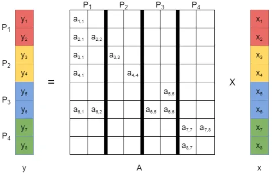
In this thesis, as a kernel application, column-parallel Sparse Matrix-Vector Mul-tiplication (SpMV) is used. The term sparse matrix is used when the ratio of nonzeros to the total size of the matrix is very small, and especially much smaller than the ratio of zeros to the total size of the matrix. During SpMV applications, only the nonzeros of the sparse matrix will be multiplied with the corresponding element on the vector, since zeros will not add to the total of the multiplied row. On distributed-memory systems, for column-parallel SpMV, nonzeros of the sparse matrix are partitioned among different processor based on their columns. A sample 4-way partitioning of 8×8 A matrix on four processors is given in Figure 2.1. In the figure, multiplication of y = Ax is shown and the nonzeros in matrix A are indicated by ai,j. Each of the four different processors stores the data of nonzeros of two columns of A. Processors perform all computations associated with the nonzeros assigned to them according to owner computes rule. Also each processor is responsible for computing the results for two y-vector elements. The colors represent the y-vector elements which are calculated by each processor: red for P1, yellow for P2, blue for P3 and green for P4. x-vector elements are colored
in a similar way assuming a conformable input output partition. That is xi and yi are assigned to the same processor.
Figure 2.1: Column-parallel SpMV example for y = Ax on four processor system where A is a 8 × 8 square matrix.
Because of the columnwise partitioning, each processor already owns x-vector elements that are needed for its local computations. So there is no communication on x-vector elements. However, reduce type of communication might be needed in the final computation on some of the y-vector elements. For example, P1 and P3 compute local partial results for y6by respectively performing the scalar multiply-add operations y1
6 = a6,1× x1+ a6,2× x2 and y36 = a6,5 × x5 + a6,6× x6. Since y6 is assigned to P3, processor P1 will send y61 to processor P3 for computing the final result y6 = y16 + y63. On the other hand, computation of y1, y2, y5, y7 and y8 do not incur any communication since all nonzeros of respective rows are already assigned to the processor which is held responsible for computing the respective y element.
This initial partitioning is done using PaToH (Partitioning Tool for Hypergraphs), which is a tool developed by C¸ ataly¨urek and Aykanat, as a preprocessing step for our work [3]. With the usage of PaToH, the initial partitioning is optimized.
2.2
Communication Matrix and Compressed
Row Storage Format
As the result of the communication mentioned in the previous section, a commu-nication matrix is obtained. The input of our algorithm presented in this thesis is the communication matrix. This is a square matrix that has the same size with the number of processors in the system. Each entry in the matrix represents the volume of communication from one processor to another. Assume that the communication matrix is shown with B. If entry bij = v, then the volume of communication from processor i to processor j is v. Note that the number of messages from processor i to processor j is 0 if Bij = 0, and is 1 otherwise. The communication matrix for a SpMV application itself may also be a sparse matrix. Since our input is the communication matrix and we need to perform retrieve operations frequently, an efficient way to store the communication matrix must be implemented. There are various storage methods proposed for efficiently storing sparse matrices and Compressed Row Storage (CRS) is the one we used in this work.
In CRS format, three arrays are needed to store the matrix;
• An array to store all nonzeros in the sparse matrix in row-major order • An array to store column index of each nonzero
• A pointer array which stores starting index of each row
Note that the third array allows access for both the starting and the ending index for each row. The starting index for processor i is just one more than the ending index for processor i − 1. In our algorithm, the first array represents the volume of messages and the second array corresponds to the receiver processors of the messages.
B = 0 2 0 0 5 0 0 3 1 0 0 6 0 0 2 0
For the B matrix given above, corresponding CRS format storage will be as following;
Value array 2 5 3 1 6 2
Column index array 2 1 4 1 4 3 Pointer array 0 1 3 5 6
Figure 2.2: CRS storage format for matrix M
Here second entry in pointer array shows that the nonzeros of the second row start at index 1 of the other arrays. When that index is checked, column index of 1 and the value of 5 is observed. This indicates that entry B2,1 = 5.
The efficiency of CRS format depends on the ratio of nonzeros. Sizes of the first two arrays are equal to the number of nonzeros in the matrix and the size of the third array is equal to the number of processors plus one. That extra space allows keeping track of the ending index of the last element. Compared to the default storage format, which requires n2 space for a system with n processors, CRS format only requires 2 · nonzeros + n + 1 space. Since the ratio of nonzeros
n is assumed to be very small in sparse matrices, CRS storage format is efficient.
2.3
Terminology and Problem Statement
In point-to-point communication, each processor has a set of processors that it is sending messages to. Assuming that the communication matrix is stored in CRS format, this set can be obtained using the pointer array to obtain a range on the column index array. All elements in this range are the target processors. For processor i, this range is from the ith element of the pointer array to the
(i + 1)th element of the pointer array, exclusive. The entries falling in this range in the column index array show the target processors for processor i and the set containing these processors is denoted as SendSet(i).
With the definition of outgoing message set given above, another important aspect is the size of this set. The size of set SendSet(i) is shown as |SendSet(i)| or shortly |SS(i)| and defined as the number of outgoing messages of processor i. Until now, the communication term is used only for direct communication and a message from processor i to processor j is shown as mi,j. However, our algorithm results in indirect messages that is sent to the target processor via an intermediate processor. In these cases, m is used to indicate the direct message between two processors as mentioned and M is used to indicate a combined message, which contains one or more direct messages.
Figure 2.3: An example to denote the difference between direct message m and combined message M .
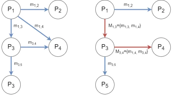
In Figure 2.3, an example is given for a system with five processors. In this example, only processors P1 and P3 are sending messages and their send sets are SendSet(P1) = {P2, P3, P4}, SendSet(P3) = {P4, P5} as shown on the left side of the figure. Messages m1,2 and m3,5 are sent directly. However, message m1,4 is combined with m1,3 and encapsulated in M1,3. The combined message can be denoted as M1,3 = {m1,3, m1,4}. On the right side of the figure this is shown where
blue arrows denote direct messages and red arrows denote combined messages. When the combined message M1,3 is received by processor P3, message m1,3 is arrived its target, but message m1,4 must be sent to processor P4. Here it is combined with message m3,4 as M3,4 = {m1,4, m3,4}. In this thesis, we call this process as message sharing from processor P1 to processor P3 and the shared message is m1,4. Note that combining messages does not increase the number of messages sent by a processor, however it increases the total volume sent by a processor.
In this work, we aim to decrease latency through message combining and sharing. Our main target is reducing the number of messages sent by the maximally-loaded processor, since it is the bottleneck in latency-bound applications. The input of our algorithm is a processor-to-processor communication matrix and we try to achieve the reduction in latency by reorganizing the communication between processors.
Chapter 3
Related Work
3.1
Reducing Communication Overhead and
Communication Cost Metrics
In parallel applications, the overhead resulting from communication between pro-cessors is a bound on the performance. There are numerous works in the litera-ture, aiming an improvement on processor-to-processor communication overhead. Some of these works include partitioning models and most of these models also aim to maintain the computational load balancing while reducing the overhead [4, 5, 6, 7].
In these works, different communication cost metrics are considered. U¸car and Aykanat [5] used a two-phase methodology involving hypergraph partitioning to address the communication cost metrics of total volume, total message count and maximum volume. Bisseling and Meesen [6] proposed a greedy algorithm to minimize the maximum send and receive volume loads of processors. Their approach is also a two-phase approach, where in the first phase they reduce total volume and in the second they reduce maximum volume while respecting the volume attained in the first phase. Acer et al. [7] investigates graph and hypergraph partitioning methods to address volume-related communication cost
metrics. Their approach relies on the recursive bipartitioning framework and uses a flexible formulation based on utilization of additional weights for vertices to address cost metrics such as maximum send volume, maximum receive volume, maximum sum of send and receive volume etc. In our work, we consider the maximum number of messages sent by a processor and the average number of messages per processor in the system as communication cost metrics.
3.2
Using Neighborhood Collectives
There are also various works using the sparse neighborhood collective opera-tions [8, 9, 10, 11, 12, 13, 14, 15, 16, 17]. Sparse collective operaopera-tions first pro-posed by Hoefler and Tr¨aff [11]. They define three sparse collective operations: sparse gather operation, sparse all-to-all operation and sparse reduction opera-tion. Later, MPI Forum simplified and renamed these operations as neighborhood collective operations [12]. Hoefler and Schneider proposed further improvements and optimizations for neighborhood collective operations [12].
Tr¨aff et. al. proposed an efficient way to implement sparse collective communica-tions on isomorphic settings [8]. Their proposed approach allows faster setup times if the processes are assumed to have identical, relative neighborhoods. Renggli et. al. used the sparse communications to propose an efficient framework for distributed machine learning applications [10].
Message-combining algorithms are first proposed by Tr¨aff et. al. [13]. However, their work focuses only on isomorphic communication patterns. Further improve-ments and generalizations are done by Ghazimirsaeed et. al. [14]. The authors propose a framework to reduce the total number of messages in the system by exploiting the common messages between processors. This is very similar to our work, however Ghazimirsaeed et. al. fixes the number of processors in a group during message sharing. For example, if that fixed number is chosen as four, there would be four processors in every group and each processor shares messages with other group members. In our work, we remove this constraint.
3.3
Store-and-Forward Framework
A recent work by Selvitopi and Aykanat proposed a store-and-forward (STFW) approach for reducing the latency [4]. In this work, the processors are organized into a virtual process topology (VPT) inspired by the k-ary n-cube networks. In an n-dimensional VPT, each processor has n value representing its coordinate in each dimension and two processors are called as neighbors if they share the same coordinates in all dimensions except one. So, processors Pi and Pj are called neighbors in dimension d if;
(Pd
i 6= Pjd) ∧ (Pic= Pjc, 1 ≤ c 6= d ≤ n)
In a VPT, direct communication between neighbors is allowed. However, a pro-cessor might be sending messages to another propro-cessor, which is not its neighbor. In these cases the message must be stored in an intermediate processor and for-warded to the target processor. An example for this is given in Figure 3.1, for a 2-dimensional VPT that has 9 processors. In the figure two messages are shown: mP1,P3 and mP1,P9. The message mP1,P3 can be sent in a direct communication
since P1 and P3 are neighbors. However, same can not be applied for the message mP1,P9. Instead, this message can only be sent via an intermediate processor, P7.
In this example, the message is stored in P7 and then forwarded.
This work by Selvitopi and Aykanat achieved a reduction in both the number of outgoing messages sent by the maximally-loaded processor and the average number of messages sent by a processor in the system, at the expanse of average message volume sent by a processor. However, in latency-bound applications, the message volume is not a major concern. In our work, we take this work of Selvitopi and Aykanat as baseline. In Chapter 6, we used same data sets and compared our results with this work.
Figure 3.1: A 2-dimensional VPT example for 9 processors. Message mP1,P3 is
Chapter 4
Message Sharing Utilizing the
Common Outgoing Messages
In this chapter, we provide a detailed message-sharing-based algorithm that re-duces the number of messages sent by the maximally-loaded processor. In a single iteration, we pair the maximally-loaded processor with another processor in order to reduce the number of outgoing messages of the maximally-loaded processor. We call this process as message sharing. In the next iteration, a new maximally-loaded processor (which may be same with the previous one) is again paired with another processor. This iterative approach will continue until there is no decrease in the number of outgoing messages of the maximally-loaded processor despite the message sharing. Eventually, the message load of the maximally-loaded pro-cessor in the system will be decreased, resulting in an improvement in latency bottleneck.
The rest of this chapter is organized as follows: in Section 4.1 general message sharing scheme between two processors is given. In Section 4.2, this general scheme is specified for the maximally-loaded processor. Lastly, in Section 4.3 the iterative nature of the algorithm is discussed along with the data structure and future changes as the message sharings occur.
4.1
Sharing of Common Messages
In this section, we define the general message sharing scheme by exploiting the common outgoing messages. Assume that the message sharing will occur between processors Paand Pb, and their outgoing message sets are defined by SendSet(Pa) and SendSet(Pb) respectively. We refer them as pair processors. In order to reduce either |SS(Pa)| or |SS(Pb)| (or both), we exploit their common outgoing message set C, where C = SendSet(Pa) ∩ SendSet(Pb) and the size of this set is |SS(C)|. The aim of message sharing is creating new send sets SendSet0(P
a) and SendSet0(Pb) where each processor in common outgoing message set C is present in either SendSet0(Pa) or SendSet0(Pb). This means;
∀Px ∈ C : (Px ∈ SendSet0(Pa) ∧ Px ∈ SendSet/ 0(Pb)) ∨ (Px ∈/ SendSet0(Pa) ∧ Px ∈ SendSet0(Pb))
must be true. In other words, after message sharing, only one of the pair proces-sors will be sending a message to each processor in set C.
As an example; consider Pt∈ SendSet(Pa)∧Pt ∈ SendSet(Pb), which also means Pt∈ C. After message sharing Ptwill be either in SendSet0(Pa) or SendSet0(Pb), but not both. Lets assume Pt ∈ SendSet0(Pa), so the messages to processor Pt will be sent by processor Pa. Here, processor Pb will send its own message mPb,Pt
to Paso that it can be combined with processor Pa’s original message mPa,Pt. Now
the combined message MPa,Pt = {mPa,Pt, mPb,Pt} can be sent by processor Pa to
processor Pt. Here Pa acted as the intermediate processor for the communication from Pb to Pt. In this given message sharing example, |SS(Pb)| is reduced by one. It must be noted that if Pa ∈ SendSet(P/ b), then Pa must be included in SendSet0(Pb) resulting in an increase of one in |SS(Pb)|. However, this overhead will be ignored since the pair processors will be sharing more than one message. Further experiments and analysis prove that this overhead is, in fact, relatively small. This will be addressed in Chapter 6 (see Table 6.5).
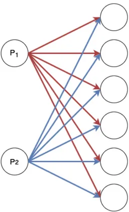
Figure 4.1: A communication example where |P1| = |P2| = 6 and SendSet(P1) = SendSet(P2)
two processors with exactly same outgoing message sets are shown. Outgoing messages of P1 are shown with red arrows and outgoing messages of P1 are shown with blue arrows. After message sharing, it is enough for both processors to send only half of their original outgoing messages, and share the remaining ones with their pair.
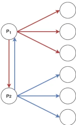
This is shown in Figure 4.2, where P1 sends messages of P2 along with its own messages to the upper half of the receiving processor in the figure. Here the red arrows also contain the messages of P2 which were supposed to be sent to those processor in the upper half. P1 acts as an intermediate processor for these messages of P2. Note that although the processors share three of their messages with each other, the reduction in their send set size is in fact two, with the addition of the overhead resulting from sending messages to each other.
Figure 4.2: Resulting communication of Figure 4.1 after message sharing
4.2
Message Sharing for the Maximally-Loaded
Processor
In our algorithm, message sharing is mainly used for reducing the message load of the maximally-loaded processor. We will refer to this processor as Pmax. For this purpose an iterative method is applied, where at each step, Pmax is paired with another processor, Pf riend. They will share their messages as explained in section 4.1. After the message sharing, |SS(Pmax)| will be reduced as some of its outgoing messages will be sent via Pf riend, and a new Pmax will be chosen (which might still be the same processor). The processor Pf riend will be chosen among the other processors in the system based on the criteria of number of its common messages with Pmax.
Pmax∈ P : |SS(Pmax)| ≥ |SS(Pi)|, ∀Pi ∈ P
The pair processor for Pmax, Pf riend, will be chosen as:
Pf riend ∈ (P − Pmax) : |SendSet(Pf riend) ∩ SendSet(Pmax)| ≥ |SendSet(Pi) ∩ SendSet(Pmax)|, ∀Pi ∈ (P − Pmax)
At each iteration of our algorithm, Pmax and Pmin are chosen according to above criteria. This choice of Pf riend results in the most possible send set size decrease in the system, since the decrease in |SS(Pmax)| + |SS(Pf riend)| will be equal to |SendSet(Pf riend) ∩ SendSet(Pmax)| and our choice maximizes it. It must be noted that the choice of Pf riend may not result in the most possible reduction for the current Pmax. However, since our method is an iterative one, future steps (i.e. future maximally-loaded processors) must be also considered and if needed, |SS(Pf riend)| should also be reduced.
To achieve the best results, our algorithm aims to assign the shared messages in such a way that |SS(Pmax)|0 = |SS(Pf riend)|0 is achieved at the end of the sharing, where |SS(Pmax)|0 represents the size of SendSet0(Pmax). This might not be possible and the alternatives is discussed in the following subsections.
4.2.1
Equal Sharing not Possible
During message sharing, send set sizes are always decreasing and the main aim is decreasing the send set size of maximally-loaded processor, Pmax. However, as explained in section 4.2, our algorithm also decreases the send set size of pair processor of Pmax, Pf riend, if opportunity arises. On the other hand, if the difference between send set sizes of Pmaxand Pf riendis large enough, our algorithm ignores |SS(Pf riend)| and solely tries to decrease |SS(Pmax)|.
In order to decide this, the set of common outgoing messages, C = SendSet(Pf riend) ∩ SendSet(Pmax), must be defined. The size of this set is
|SS(C)|. If |SS(Pmax)| > |SS(Pf riend)| + |SS(C)|, then it can be inferred that it is not possible to achieve equality by message sharing. The reason is that the de-crease in |SS(Pmax)| may be as much as the size of common outgoing message set (ignoring the possible overhead of one if Pf riend ∈ SendSet(P/ max)). As a result, even if Pmax shares all of the common messages, |SS(Pmax)|0 > |SS(Pf riend)|0 will be true. Still, the algorithm follows this approach, since it is clear that |SS(Pf riend)| is not a concern for this iteration. So for this case, Pmax will remove all of the messages in C from its send set and the resulting send sets will be;
SendSet0(Pf riend) = SendSet(Pf riend) and SendSet0(Pmax) = SendSet(Pmax) − C
This results in;
|SS(Pf riend)|0 = |SS(Pf riend)| and |SS(Pmax)|0 = |SS(Pmax)| − |SS(C)|
4.2.2
Equal Sharing Possible
For the sharing scheme explained in the previous subsection, required condition is |SS(Pmax)| > |SS(Pf riend)| + |SS(C)|. If the condition is not satisfied, then this sharing scheme will result in |SS(Pf riend)|0 > |SS(Pmax)|0. So, contrary to previous scheme, assigning all of the common messages to |SS(Pf riend)| will not be efficient in this case, since |SS(Pf riend)| might be very close |SS(Pmax)|. In fact, even the case |SS(Pf riend)| = |SS(Pmax)| is not infrequent in our experi-ments. Since, |SS(Pf riend)| might be large as well, the aim for this case is making |SS(Pmax)|0 and |SS(Pf riend)|0 equal after the message sharing. This can be done by assigning α of the common messages to |SS(Pf riend)| where;
α = |SS(C)| + |SS(Pmax)| − |SS(Pf riend)|
Here α also donates the amount of reduction in |SS(Pmax)|, i.e. |SS(Pmax)|0 = |SS(Pmax)| − α.
As a result, Pf riend will share |SS(C)| − α number of its messages to Pmax, thus |SS(Pf riend)|0 = |SS(Pf riend)| − |SS(C)| + α. Note that if |SS(C)| + |SS(Pmax)| − |SS(Pf riend)| is even, then |SS(Pf riend)|0 = |SS(Pmax)|0 is obtained. In the cases where |SS(C)| + |SS(Pmax)| − |SS(Pf riend)| is odd, it is rounded down when dividing by two. This results in |SS(Pmax)| = |SS(Pf riend)| + 1 after the sharing. To further clarify the methodology explained, we provide an example. Con-sider a scenario where |SS(Pmax)| = 100 and |SS(Pf riend)| = 80. If the size of their common outgoing message set C is equal to 10, then |SS(Pmax)| > |SS(Pf riend)| + |SS(C)| and equal sharing is not possible. So Pmax will share all of these ten messages with Pf riend and reduce its send set size by ten, resulting in |SS(Pmax)|0 = 90 and |SS(Pf riend)|0 = 80 (since Pf riend does not share any message, its send set size is not changed). However, if |SS(C)| = 40, then equal sharing is possible. According to Equation 4.1, α = 30 is obtained. This indicates that thirty messages should be shared from Pmax to Pf riend and remaining ten messages in common outgoing set should be shared from Pf riend to Pmax. The resulting send set sizes will be |SS(Pmax)| = |SS(Pf riend)| = 70.
4.3
Multiple Message Sharings and Grouping
In the previous section, a general message sharing scheme is proposed and ex-plained. Our algorithm iteratively uses this scheme to reduce the message load of maximally-loaded processor (Pmax). The iterations will continue until there is no further decrease in the message load of the maximally-loaded processor. This stopping condition will be triggered when the same processor is chosen as Pmax in two consecutive iterations with the same |SS(Pmax)|. The reason for this is the overhead that occurs during message sharing if the paired processor Pf riend is not included in SendSet(Pmax). This overhead creates one extra message for Pmax and if the message sharing does not result in a further reduction, it increases the
load instead of decreasing it. It must also be noted that if the algorithm continues at this point there is a possibility to reduce the load of other processors in the system. However, since the latency runs into bottleneck by the maximally-loaded processor there is no need to continue unless the load of the maximally-loaded processor is decreased.
It is also possible that the same processor might become the maximally-loaded processor or pair of another maximally-loaded processor multiple times, with different send set sizes. In these cases, the processor’s original send set and the actual send set usually differ. It might have shared some of its original outgoing messages in the previous iterations and removed them from its send set, thus decreasing the actual send set size.
To handle this situation, we propose an algorithm that always uses the initial send sets for each processor in a static way. Although the send sets are updated at each iteration, the number of common outgoing messages between two processors and the pairings are decided according to the initial send set. Yet, the send set size for each processor is kept dynamically for deciding the maximally-loaded processor. The reason for keeping and using a static list for initial send sets is that; if two processor have a common outgoing message, although one of them removed that message from its send set in a previous iteration, that message can still be shared between these processors. Consider that Pa and Pb are paired and they both send a message to Pz. Also consider that in a previous iteration Pa was paired and shared messages with Pc, such that Pz ∈ SendSet0(Pc) ∧ Pz ∈ SendSet/ 0(Pa). This means that the message mPa,Pz will be sent to Pz in combined message MPc,PZ.
Our algorithm allows Pato share the message mPa,Pz with Pb in current iteration.
This will result in,
Pz ∈ SendSet0(Pb) ∧ Pz ∈ SendSet/ 0(Pa) ∧ Pz ∈ SendSet/ 0(Pc)
However, it must not considered as the message mPa,Pz is transferred from Pa to
Pc, and then from Pc to Pb. No message transfer is made until our algorithm fully finishes. So the message mPa,Pz will be transferred to Pb, which will send
the message to Pz in combined message MPb,Pz.
Algorithm 1 Iterative Message Sharing for Latency Reduction
Require: A set of n processors and their outgoing message sizes in array outgoingSize
1: prevM ax = −1, prevM axSize = −1 2: max = 0, Pmax = 0
3: while (prevM ax 6= Pmax) ∨ (prevM axSize 6= outgoingSize[Pmax]) do 4: for i ← 0 to n do
5: if outgoingSize[i] > max then 5: max ← outgoingSize[i]
5: Pmax ← i
6: end if 7: end for
8: prevM ax ← Pmax, prevM axSize ← outgoingSize[Pmax]
9: Find Pf riend that has the most common outgoing messages with Pmax 10: Share messages between Pf riend and Pmax
11: Update outgoingSize[Pmax] and outgoingSize[Pf riend] 12: end while
Algorithm 1 provides the general outline of Phase I of our algorithm. The vari-ables prevM ax and prevM axSize is used to determine the stopping condition. When the maximally-loaded processor and its send set size remain same as the previous iteration, then it is obvious that the algorithm can not further reduce the number of outgoing messages of the maximally-loaded processor. This also indicates that the latency can not be further reduced and the first phase of our algorithm ends.
The loop in Line 3 to 7 is used for finding the maximally-loaded processor. Here a linear runtime approach is used, since n, the number of processors in the system, is not likely to be large. After finding the maximally-loaded processor, in Line 8 the variables are recorded for detecting the stopping condition as mentioned. After finding the maximally-loaded processor, a pair processor for it must be found as well. This is indicated in Line 9 and the details for this process is given in the next subsection. Lastly, after message sharing |SS(Pmax)| and possibly |SS(Pf riend)| are decreased. The update in Line 11 allows the algorithm to use their actual send set sizes when determining the maximally-loaded processor in future iterations.
4.3.1
Storing the Send Sets and the Data Structures
Our algorithm takes the processor-to-processor communication matrix of the ap-plication as input and uses CRS format to store that matrix since the it is expected to be a sparse matrix. The processors referred as integers ranging from 0 to n − 1, where n is the number of processors the parallel application uses. Here, processor 0 and P0 used interchangeably. Each processors outgoing message list is stored in ascending order. This allows easier implementation and runtime efficiency during both finding the number of common messages and message sharing between two processor.
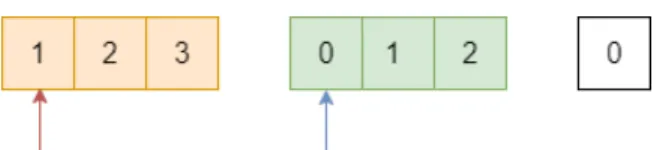
An example for n = 4 is given in Figure 4.3. In the figure, the array adja-cency represents the column indices (explained in Section 2.2) in CRS format of the processor-to-processor communication matrix and the array adjacencyPtr represents the pointers showing the starting point of each processors outgoing message set. The value array in CRS format contains the volume of communi-cation between processor and is omitted in this part, since the volume is not a major concern in our work. It must be noted that the example is given as a dense communication matrix due to the small choice of n. This kind of a dense communication matrix is unexpected in real applications.
Figure 4.3: Example for storing communication matrix in CRS format with n = 4 The ascending order of outgoing message set allows easier calculation of the num-ber of common messages a pair of processors have. Here we use a mergesort-like comparison, starting from the elements the pointers corresponding to the com-pared processors show and moving to the subsequent element of the lower element if they are not equal.
As an example consider the comparison between processor P0 and processor P3, shown with yellow and green colors respectively in the Figure 4.3. The outgoing message sets are SendSet(P0) = P1, P2, P3 and SendSet(P3) = P0, P1, P2. Initial comparison is between the first elements of the sets; P1 and P0 respectively. By the ordering of the corresponding integer, it can be said that P0 comes before P1. Since here P0 ∈ SendSet(P3), the next element in SendSet(P3) must be taken to the comparison now. The next element is P1, which is same as the current element from SendSet(P0). This indicates that there is a common outgoing message of P0 and P3, and target of those messages are P1. Now the comparison should continue with the next elements of both sets and the number of common outgoing messages for this pair should be incremented by one. A full example of this comparison in given in Figure 4.4. In the figure, finding the number of common outgoing messages of P0 and P3 is given, whose outgoing message sets are shown with yellow and green respectively. Red pointer is used for tracing the list of P0 and blue pointer is used for tracing the list of P3. The rightmost integer denotes the detected number of common outgoing messages up to that step. As can be seen from the example, once the communication matrix is compressed in CRS format and the outgoing message sets are stored in order, number of com-mon outgoing messages between two processors can be calculated in linear-time with the number of the nonzeros in the communication matrix. Since this opera-tion is used frequently in our algorithm, its running time efficiency is important. Note that this storage format is static and only stores the initial state of the communication matrix, ignoring the changes occurring to the matrix as a result of message sharings.
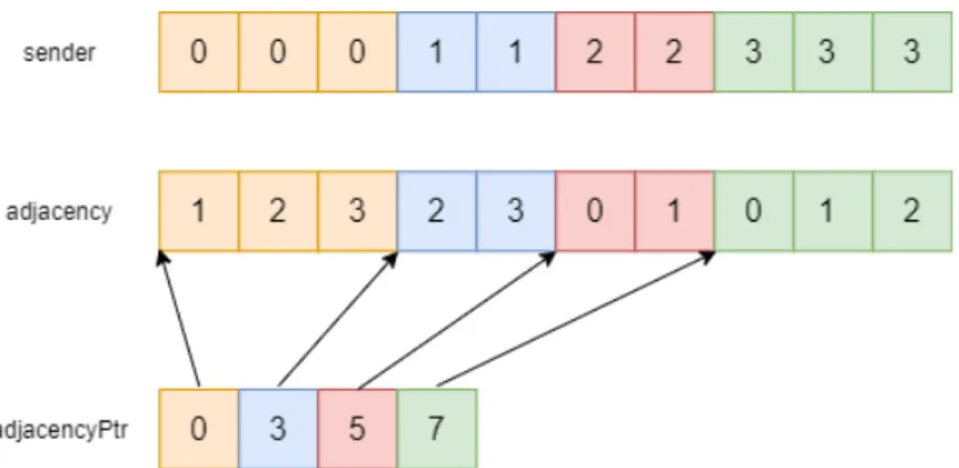
In order to keep track of the sharings, we use another parallel array denoted as sender, that has the same size as the adjacency array mentioned in Figure 4.3. It must be noted that the size of the array adjacency is equal to the total number of messages in the system and each element in this array represent one message. This newly defined sender array keeps track of which processor will be sending which message. There will be an element corresponding to every single message in this array. In Figure 4.5, an updated version of Figure 4.3 is shown, with the addition of the initial state of sender array.
Figure 4.4: Step by step example of finding the number of common outgoing messages of a pair of processors.
Combined with adjacency and adjacencyPtr arrays, sender array provides infor-mation about the communication in the system. For an integer x, adjacency[x] denotes the target processor of a message. The entry in sender[x] denotes the processor sending this message. However, this might not be the original sender. The original sender is processor Pi that is satisfying;
(adjacencyP tr[i] ≤ x) ∧ (adjacencyP tr[i + 1] > x)
Assume that adjacency[x] = k and sender[x] = j. This indicates that the mes-sage mentioned here is mPi,Pk and the processor Pj acts as the intermediate
processor for this message. Eventually this message will be sent to the target processor Pk by the combined message MPj,Pk.
Figure 4.5: Updated version of Figure 4.1, including sender array
4.3.2
Groupings
As shown in previous sections, it is necessary to identify the situation of proces-sors when they are paired. The key point here is determining whether a processor was paired with another processor in a previous iteration or not. We call those processors who has not been paired with another processor as singleton proces-sors. The importance of identifying whether the processor is singleton or not is that; if the processor is not singleton, then it might need to share some of the messages it shared in previous iterations, as explained in Section 4.3. This arises the need to keep the information about previous sharings and a possibility to change the intermediate processor for a message if needed. There are four differ-ent cases our algorithm needs to handle, depending on the singleton situation of the pair processors;
Case 1: Singleton to Singleton
The most trivial and the basic case to handle is when both processors in the pairing are singleton. For this case, the message sharing scheme explained in Section 4.2 is directly applied.
Algorithm 2 demonstrates the process of Singleton to Singleton message sharing. As an input it takes the processor pair Pmax and Pf riend with their send sets SendSet(Pmax) and SendSet(Pf riend), along with the necessary lists adjacency,
Figure 4.6: Singleton to Singleton pairing
adjacencyP tr and sender, which are stored as 1-D arrays. As the initial step α, the number of messages that will be shared by Pmax, is calculated based on the send set sizes of Pmax and Pf riend, and the size of their common outgoing message set. Note that α calculated in Line 3 is equal to α in the Equation 4.1.
In Line 5, the variables i and j are used as pointers to iterate over the outgoing message sets of Pmax and Pf riend respectively. adjacencyP tr array keeps the indices of starting elements of outgoing message sets and initial values of i and j are determined using this array. The variable msgShared is used to keep track of how many messages are shared between this pair. It helps to determine the direction of sharing, since Pmax is supposed to share α number of messages, first α sharing will be from Pmax to Pf riend and the rest will be from Pf riend to Pmax. This is determined by the check in Line 8.
The if condition in Line 7 and the corresponding else part in Line 16 to 20, demonstrates the usage of mergesort-like comparison described in Figure 4.4. If same processor is found by two pointers, then the condition in Line 7 becomes true and message sharing is done in Line 8 to 17. If Pmaxis sharing the message to Pf riend, then the element corresponding to the message in sender array becomes Pf riend, indicating that the message will be sent to the target processor by Pf riend. This decreases the send set size of Pmax by one and this is shown in Line 10. The converse is true if the message is shared from Pf riend to Pmax.
If the pointers point to different processors then the pointer pointing to the smaller element should be incremented by one, as in Line 19 or Line 20. Since the outgoing message sets are kept in an increasing order, these increment operations will result in finding all of the same elements in outgoing message sets of Pmax and Pf riend. The stopping condition of this message sharing is triggered when one
of the pointers is gone beyond the range of the outgoing send set of corresponding processor. This happens when either i is equal to the first element of the processor Pmax+ 1 or j is equal to the first element of the processor Pf riend+ 1. Note that the condition for last processor is different and instead of the first element of the next processor, the end of the list is checked. However, this is not included in Algorithm 2, for simplicity.
Algorithm 2 Singleton to Singleton Message Sharing
Require: Two integers representing processors Pmax and Pf riend, their send sets, their send set sizes |SS(Pmax)| and |SS(Pf riend)|, adjacency, adjacencyP tr and sender arrays
1: C ← SendSet(Pmax) ∩ SendSet(Pf riend) 2: if |SS(Pf riend)| + |SS(C)| ≤ |SS(Pmax)| then 2: α ← |SS(C)|
3: else
3: α ← |SS(C)| + |SS(Pmax)| − |SS(Pf riend)| 2
4: end if
5: i ← adjacencyP tr[Pmax], j ← adjacencyP tr[Pf riend], msgShared ← 0 6: while (i < adjacencyP tr[Pmax+ 1]) ∧ (j < adjacencyP tr[Pf riend+ 1]) do 7: if adjacency[i] = adjacency[j] then
8: if msgShared < α then 9: sender[i] ← Pf riend 10: |SS(Pmax)| ← |SS(Pmax)| − 1 11: else 12: sender[j] ← Pmax 13: |SS(Pf riend)| ← |SS(Pf riend)| − 1 14: end if 15: msgShared ← msgShared + 1 16: i ← i + 1 17: j ← j + 1 18: else
19: if adjacency[i] < adjacency[j] then 19: i ← i + 1 20: else 20: j ← j + 1 21: end if 22: end if 23: end while
Case 2: Singleton to Non-singleton
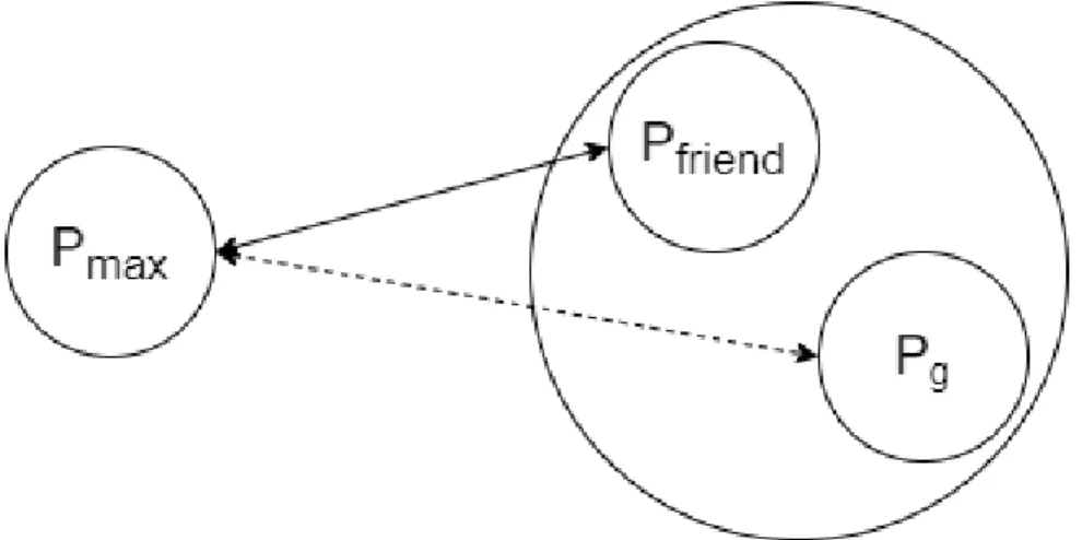
When Pf riend is not singleton, this indicates that it has shared some messages in previous iteration. For this iteration, before message sharing between Pmax and Pf riend, we can exploit the previous sharings of Pf riend. Without loss of generality, assume that Pg is one of the processors Pf riend was paired in a previous iteration. We define as Pf riend and Pg are in the same group. There might be a processor Pz, which receives messages from Pmax, Pf riend and Pg, i.e;
Pz ∈ SendSet(Pmax) ∧ Pz ∈ SendSet(Pf riend) ∧ Pz ∈ SendSet(Pg)
Further assume that during the previous sharing Pf riend shared its message to Pz with Pg, and removed it from its send set, resulting in;
Pz ∈ SendSet0(Pg) ∧ Pz ∈ SendSet/ 0(Pf riend)
Since we consider initial send sets SendSet(Pmax) and SendSet(Pf riend), not the actual send sets SendSet0(Pmax) and SendSet0(Pf riend) when comparing the common messages, and since Pz is included in both SendSet(Pmax) and SendSet(Pf riend), it is counted towards their total common messages and con-tributed to the choice of selecting Pf riendas the pair of Pmax. However, it is not in the actual send set of Pf riend, so if Pmaxshared the message to Pz with Pf riend, this will result in an extra message for Pf riend and will cause overhead. On the other hand, Pz is a common target for both Pmax and Pg, and also Pz ∈ SendSet0(Pg). Thus, Pmax can share its message mPmax,Pz with Pg, and processor Pg can send
the combined message MPg,Pz = {mPmax,Pz, mPf riend,Pz, mPg,Pz} to Pz.
When this process is finished and Pmax shared as much as it can share with previous group members (possible more than one) of Pf riend, then the next step is similar to Case 1 and the sharing between two processors are done as explained in section 4.2. One thing to note is that if there is an opportunity to equally share, then the number of message to be shared from Pmax to Pf riend, α, has to
Figure 4.7: Singleton to Non-Singleton pairing
be calculated considering the current send set size of Pmax. This means that the messages shared in the first part of this case (sharings between Pmax and other group members of Pf riend) must be reduced from send set size of Pmax. This may result in a possible equal sharing between Pmax and Pf riend, although it was not possible when they are initially paired (since |SS(Pmax)| is decreased). In these situations sharings will be done according to scheme explained in section 4.2.2, not in section 4.2.1.
Case 3: Non-singleton to Singleton
When Pmax is a non-singleton processor, the approach is similar to Case 2. Just as exploiting the previous sharings of Pf riend in Case 2, we exploit the previous sharings of Pmaxin this case. Firstly, Pf riendshares messages with group members (i.e. the processors Pmax was paired in previous iterations) of Pmax and then two paired processors, Pf riend and Pmax, share messages. Similar to Case 2, after first step |SS(Pf riend)| must be updated and the equal sharing condition must be checked again. However, contrary to Case 2, for this case the possible scenario is that the equality may become impossible, although it was possible in the initial pairing of Pmax and Pf riend.
Figure 4.8: Non-Singleton to Singleton pairing
One other thing to note for Case 2 and Case 3 is that, during message sharing be-tween Pmax and Pf riend, the non-singleton one should avoid sharing the messages that will be sent to the processors in its group. As an example consider that Pmax is a non-singleton processor that has processor Pg in its group and Pf riend is a singleton processor (Case 3). Also consider that the equal sharing between Pmax and Pf riend is not possible, so all message transfers would be from Pmax to Pf riend. If Pg ∈ SendSet(Pmax) ∧ Pg ∈ SendSet(Pf riend), then Pg should be removed from SendSet(Pmax) and the message mPmax,Pg should be sent by Pf riend. However,
since Pmax and Pg are in the same group, they must have been paired during a previous iteration and it is very likely that Pmax shared some message with Pg. Assume that Pz is a target of this kind of a message. This indicates that the message mPmax,Pz will be contained in combined message MPg,Pz. During current
iteration, if Pmax shares the message to Pg with Pf riend, then indirectly it shares the message to Pz as well as any other message it has shared with Pg during their pairing. Since Pz ∈ SendSet(Pf riend) is not guaranteed, the sharing of Pg to Pf riend will result in unnecessary overhead. This overhead will occur even if only one such processor is not included in SendSet(Pf riend) and it is likely that Pmax shared more than one such messages with Pg. Thus, during message sharings that involve at least one non-singleton processor, the previous groupings must be considered and the non-singleton processor should avoid sharing messages that targets a processor it was grouped with.
Case 4: Non-singleton to Non-Singleton
Figure 4.9: Non-Singleton to Non-Singleton pairing
When both of the paired processors are non-singleton, the approach is similar to combination of Case 2 and Case 3, with some minor changes. Initially we consider as if it is Case 2, assuming Pmax is a singleton processor and shares messages with the group members of Pf riend. However, during this process we must also consider the group members of Pmax and avoid sharing them with group members of Pf riend. This is the difference from Case 2, where Pmax is a singleton processor indeed. Then the same process is applied for Pf riend, again avoiding sharing its group members.
The last step for this case is the message sharing between Pmax and Pf riend. For this phase, actual send set sizes of these two processors and their common set size are calculated considering the previous steps of this case. Again during this step, they avoid sharing the messages to the processors that are in their group. Algorithm 3 outlines how to find out whether the target processor of the message to be shared is in a group or not, when there is a non-singleton processor in the pairing. This approach is applied for Case 2, Case 3 and Case 4 (twice). As explained in last part of Case 3, this is applied in order to avoid the sharing of a processor which is already in a group with the current sharing processor, either Pmax or Pf riend.
Algorithm 3 is applied when a target processor is found in the outgoing message sets both of Pmax and Pf riend, meaning that one of them can share the message it is sending to that target processor. Here this is represented in the perspective of Pmax. Note that for the algorithm explained here, it does not matter whether the Pf riend is singleton or not. If it is singleton, then a similar procedure for its potential shared messages will be applied.
There are three necessary conditions for this algorithm to apply;
• Message from Pf riend to the target processor is not being sent by Pf riend • Message from Pf riend to the target processor is not being sent by Pmax • Message from Pmax to the target processor is being sent by Pmax
This indicates that Pmax is still sending its own message and the message from Pf riend is being sent by a processor other than Pf riend or Pmax. When these conditions are satisfied, outgoing message set of the sharing processor (in this case Pmax) is traced, as in Line 2 of Algorithm 3. For each element in the outgoing message send, the corresponding sender of the message is checked. If that sender is the processor that is the target of the message to be shared, then the boolean variable inGroup is set as true and this message sharing is simply ignored. When this happens, the message sharings will continue with the next elements as in Line 16 and Line 17 of Algorithm 2.
Algorithm 3 Identifying Grouping During Message Sharing with Non-Singleton Require: Two integers representing processors Pmax and Pf riend, their send sets, pointers i and j tracing send sets of Pmax and Pf riend respectively, adjacency, adjacencyP tr and sender arrays
1: inGroup ← f alse
2: for k ← adjacencyP tr[Pmax] to adjacencyP tr[Pmax+ 1] do 3: if sender[k] = adjacency[i] then
3: inGroup ← true 4: end if
5: end for
Chapter 5
Message Sharing Between
Maximally and
Minimally-Loaded Processors
In this chapter, the second phase of our algorithm is given, which is a follow-up to the first phase explained in Chapter 4. After Phase I, a new communication matrix is calculated and used in Phase II. Again CRS format is used for this communication matrix as described in Section 4.3.1 with the same naming for convenience. The main difference of the second phase is that the maximally-loaded processor, Pmax, is paired with the minimally-loaded processor Pmin. The number of common messages between these two processors are not considered during pairing.
For the calculation of the new communication matrix, processor Pj is considered to be in SendSet(Pi) if at least one of the following is true;
• Pi itself sending its own message to Pj
• Pi has shared one of its original messages with Pj
its message mPm,Pj with Pi
The logical expressions corresponding to the above points is respectively as fol-lows;
• adjacency[k] = Pj ∧ sender[k] = Pi for adjacencyP tr[Pi] ≤ k < adjacencyP tr[Pi+ 1]
• sender[k] = Pj for adjacencyP tr[Pi] ≤ k < adjacencyP tr[Pi+ 1]
• adjacency[k] = Pj, sender[k] = Pi for adjacencyP tr[Pm] ≤ k < adjacencyP tr[Pm+ 1]
A new communication matrix is obtained using the mentioned conditions above. In CRS representation, the column indices for this communication matrix (i.e. target processors for the messages) is named as adjacency0 and the corresponding pointer matrix is named as adjacencyP tr0. Also, another parallel boolean array of the same size with adjacency0 is used to keep track of whether the corresponding message is shared in this stage or not. Lastly, the information of the received messages for the minimally-loaded processor is kept dynamically. The detailed information for these data structures are given in the explanation of algorithm 4. In Phase II, the number of messages to be shared from Pmax to Pmin, α, is calculated as;
α = |SS(Pmax)| − |SS(Pmin)| 2
With this choice of α, the number of messages after sharing, |SS(Pmax)|0 and |SS(Pmin)|0 will be equal. Similar to the first phase, with the decrease in the send set size of Pmax, a new processor is selected as the maximally-loaded processor. This process will continue until there is no decrease in the send set size of the maximally-loaded processor, at which point the algorithm finishes.
The stopping condition for the algorithm may be triggered in two ways; either send set size of each processor in the system becomes equal to the average (with the possibility of +/ − 1) or the maximally-loaded processor is not able to share messages anymore. The reason of the latter condition is that, the maximally-loaded processor Pmax, avoids sharing messages which are shared with it during a previous iteration of this phase. This approach is similar to the cases 2,3 and 4 of the first phase. Full outline of the second phase is given in Algorithm 4. In Algortihm 4, outgoingSize[Pmax] and |SS(Pmax)| used interchangeably. The initial variable declarations are similar to Algorithm 1, which provides the outline of Phase I of our algorithm. However in Algorithm 4, Pmin is also found along with Pmax. The check condition for while loop in Line 3 is same with Algorithm 1, when the send set size of Pmax can not be further reduced. Then from Line 4 to Line 9 the maximally-loaded processor and the minimally-loaded processor is found. From Line 10 to Line 12 the initialization of the variables that will be used during the next loop is done.
The while loop starting from Line 13 is the part where the message sharing happens. Here we use a helper array stillOwn to identify whether a specific message was shared in a previous iteration of this phase or not. This is a boolean array of the same size with adjacency0 array. If a message is already shared during this phase, the corresponding entry in stillOwn array is set to f alse. Thus, it is only possible a message whose corresponding entry in stillOwn array is true and Line 14 checks this boolean value.
If the message can be shared, then the corresponding entry in stillOwn array is set to f alse and send set size of Pmax is decreased by one. In Phase II, a processor avoids sharing a message it received from another processor in a previous iteration. To keep track of this, we use a dynamic list transf erredM sg which holds tuples of shared messages in this phase. In Line 17 the tuple (Pmin, adjacency0[i]) is added to the list, since Pmax shared the message to adjacency0[i] with Pmin. In a future iteration the list will be iterated and Pmin will not share the message to adjacency0[i] as it is present in the list. These checks are not included in Algorithm 4.
Although we do not consider common outgoing messages for this phase, sharing a common messages should not increase the send set size of Pmin. This is checked in Line 19 to Line 23. If the target processor for the message to be shared, adjacency0[i], is found in SendSet(Pmin), then the variable msgExist is set to true and the send set size of Pmin does not increase.
After the message sharing for a specific message is finished, the algorithm con-tinues with the next element in SendSet(Pmax). This is represented in Line 27. The algorithm finishes if all the elements in SendSet(Pmax) is checked (i.e. if i = adjacencyP tr0[Pmax+ 1]) or if Pmax shared α amount of its messages to Pmin. Note that all of the message sharings in this phase results in changes of the sender array which keeps the actual senders for each message. These changes are not included in Algorithm 4.
Algorithm 4 Phase II Outline
Require: A set of n processors and their outgoing message sizes in array outgoingSize, along with arrays adjacency0, adjacencyP tr0, stillOwn and the list transf erredM sg
1: prevM ax = −1, prevM axSize = −1 2: max = 0, Pmax = 0, min = 0, Pmin = 0
3: while (prevM ax 6= Pmax) ∨ (prevM axSize 6= outgoingSize[Pmax]) do 4: for i ← 0 to n do
5: if outgoingSize[i] > max then 5: max ← outgoingSize[i]
5: Pmax ← i
6: end if
7: if outgoingSize[i] < min then 7: min ← outgoingSize[i] 7: Pmin ← i 8: end if 9: end for 10: α = |SS(Pmax)| − |SS(Pmin)| 2
11: prevM ax ← Pmax, prevM axSize ← |SS(Pmax)|, msgShared ← 0 12: i ← adjacencyP tr0[Pmax]
13: while (i < adjacencyP tr0[Pmax+ 1]) ∧ (msgShared < α) do 14: if stillOwn[i] then
15: stillOwn[i] = f alse
16: |SS(Pmax)| ← |SS(Pmax)| − 1
17: add tuple (Pmin, adjacency0[i]) to the list transf erredM sg 18: msgShared ← msgShared + 1
19: msgExist ← f alse
20: for j ← adjacencyP tr0[Pmin] to adjacencyP tr0[Pmin+ 1] do 21: if adjacency0[i] = adjacency0[j] then
21: msgExist ← true 22: end if 23: end for 24: if !msgExist then 24: |SS(Pmin)| ← |SS(Pmin)| + 1 25: end if 26: end if 27: i ← i + 1 28: end while 29: end while
Chapter 6
Experiments and Results
For the evaluation of our algorithm we used column-parallel SpMV as kernel application since it is a frequent application in HPC. As baseline, we used a recent work of Selvitopi and Aykanat which uses STFW framework in order to reduce the latency [4]. For this reason we used the same data set with this work. The data set contains 15 different symmetric sparse matrices with different sizes and different ratios of nonzeros. The information about these matrices are given in Table 6.1. In the table, the last column ”cv”, stands for the coefficient of variation on the degrees of rows/columns and indicates the irregularity of the matrix. These matrices are obtained from SuiteSparse Matrix Collection [18]. The input of our algorithm is the processor-to-processor communication matrix that captures the communication on a distributed-memory system for SpMV op-eration for these 15 matrices. For our experiments, we used the communication matrices for a system with 512 processors. In Table 6.2, for each of the 15 ma-trices, resulting average messages and the number of messages of the maximally-loaded processor after each of the first phase and the second phase are given along with the initial values. The geometric means obtained for the values in Table 6.2 are given in Table 6.3 along with the initial state of the communication matrix and the results of the work chosen as the baseline [4].
Table 6.1: Information of the matrices used in experiments
Name # of rows/columns # of nonzeros cv
cbuckle 13,681 676,515 0.16 msc10848 10,848 1,229,778 0.42 fe rotor 99,617 1,324,862 0.29 sparsine 50,000 1,548,988 0.36 coAuthorsDBLP 299,067 1,955,352 1.50 net125 36,720 2,577,200 0.95 nd3k 9,000 3,279,360 0.26 GaAsH6 61,349 3,381,809 2.44 pkustk04 55,590 4,218,660 1.46 gupta2 62,064 4,248,286 5.20 TSOPF FS b300 c2 56,814 8,767,466 6.23 pattern1 19,242 9,323,432 0.78 SiO2 155,331 11,283,503 4.05 human gene 2 14,340 18,068,388 1.09 coPapersCiteseer 434,102 32,073,440 1.37
From Table 6.2, it can be seen that after applying our algorithm, there is a reduc-tion in the number of average messages sent by a processor. In this parameter, our improvement is even better than the baseline work by approximately 5% (see Table 6.3). Of course, applying Phase II results in an overhead for the number of average messages in the system, but that overhead is still only 2% of the average messages. In general, our two phase algorithm results in a decrease in the number of average messages in the system.
This decrease in average number of messages is important, yet the most important parameter in this work is the number of messages sent by the maximally-loaded processor, which determines the latency in the system. From Table 6.2, the decrease of the load of maximally-loaded processor for each individual test matrix can also be seen. After applying Phase I of the algorithm, there is an improvement over the initial state by 54% (see Table 6.3). However, the improvement was still much worse than the improvement of the baseline algorithm, and thus Phase II is applied, which results in 26% and 84% improvements over the baseline and the initial state respectively.
Table 6.2: Comparison of the initial average message and bottleneck processor against the results from Phase I and Phase II of our algorithm
Average messages per processor Messages of bottleneck processor
Name Initial Phase I Phase II Initial Phase I Phase II
cbuckle 7.43 7.36 7.6 62 41 8 msc10848 16.95 16.62 17.05 67 34 18 fe rotor 12.68 12.32 12.75 41 23 14 sparsine 76.21 56.87 57.01 223 80 58 coAuthorsDBLP 175.02 48.65 48.89 288 216 50 net125 106.44 52.01 52.03 209 123 53 nd3k 59.15 24.28 24.88 107 47 26 GaAsH6 75.96 25.66 26.18 227 77 27 pkustk04 18.52 17.4 17.87 101 51 19 gupta2 154.37 31.08 31.73 276 132 33 TSOPF FS b300 c2 140.93 74.29 74.31 497 249 124 pattern1 70.41 7.76 8.06 472 61 9 SiO2 156.86 23.92 25.4 298 147 26 human gene 2 393.25 30.48 30.66 511 256 114 coPapersCiteseer 102.99 46.83 47.1 226 131 48
occurred during message sharing. In Table 6.4, average overhead for each matrix is given along with the average number of messages for that matrix. Geometric mean of these overhead is 0.8, which is just 3% of the average messages.
Table 6.3: Geometric means for average of the number of messages sent by a processor and the number of messages of the maximally-loaded processor.
Algorithm Average messages Messages of maximally-loaded
Initial 65.7 187.6
Baseline [4] 28.0 41.6
After Phase I 25.7 87.0
After Phase II 26.3 30.8
Lastly, from Table 6.2 it can be seen that for most of the test matrices, the second phase of our algorithm achieved to reduce the send set size of the maximally-loaded processor to the average of the system. Only for two of the test matrices, human gene 2 and TSOPF FS b300 c2 the load of the maximally-loaded pro-cessor is larger from the average load, and this can be attributed to irregular communication scheme of these matrices (initial max messages of 511 and 497
Table 6.4: Average overhead occurred during message sharing compared to the average number of messages
Name Average Message After Phase I Average Overhead
fe rotor 12.32 0 msc10848 16.62 0 cbuckle 7.36 0.02 nd3k 24.28 0.9 pkustk04 17.4 0 pattern1 7.76 3.61 GaAsH6 25.66 0.84 sparsine 56.87 0.24 net125 52.01 1.79 coPapersCiteseer 46.83 6.15 gupta2 31.08 3.47 SiO2 23.92 1.12 coAuthorsDBLP 48.65 9.56 TSOPF FS b300 c2 74.29 0.01 human gene 2 30.48 1.27
respectively, see Table 6.3). For more regular test matrices, our algorithm success-fully achieves a load balance. Furthermore, our algorithm still achieves our main aim of decreasing the number of messages sent by the maximally-loaded processor and this is achieved in all of the test matrices, regardless of the irregularity.