IEEE TRANSACTIONS ON MICROWAVE THEORY AND TECHNIQUES, VOL. 44, NO. 5 , MAY 1996 65 1
A Robust Approach for the Derivation
of Closed-Forrn
Green’ s Functions
M.
I.
Aksun,
Member, IEEEAbstruct- Spatial-domain Green’s functions for multilayer, planar geometries are cast into closed forms with two-level ap- proximation of the spectral-domain representation of the Green’s functions. This approach is very robust and much faster com- pared to the original one-level approximation. Moreover, il does not require the investigation of the spectral-domain behavior of the Green’s functions in advance to decide on the parameters of the approximation technique, and it can be applied to any component of the dyadic Green’s function with the same ease.
I. INTRODUCTION
UMERICAL modeling of printed structures used in
N
monolithic millimeter and microwave integrated circuits (MMIC) can be efficiently and rigorously performed by em- ploying the method of moments (MOM). The MOM is based upon the transformation of an operator equation, such as integral, differential, or integro-differential operators, into a matrix equation [l]. Although the MOM is the most effi- cient numerical technique for moderate-size printed geometries (spanning several wavelengths in two dimensions), there is still need for improvement, which could be accomplished in the calculation of the matrix elements and in the solution of the matrix equation. For small geometries like those requiring couple hundreds of unknowns, the matrix-fill time could be the significant part of the overall solution time, however, for large geometries the matrix solution time will dominate the CPU time [2].In the application of the spatial-domain MOM to the solution of a mixed-potential integral equation (MPIE), one needs to calculate the Green’s functions of the vector and scalar potentials in the spatial domain where they are represented as oscillatory integrals, called Sommerfeld integrals. The eval- uation of these integrals is quite time consuming, therefore the matrix-fill time would be significantly improved if these integrals can be evaluated efficiently. Recently, a technique has been proposed to approximate these integrals analytically for a horizontal electric dipole over a thick substrate backed by a ground plane; this is called the closed-form Grleen’s functions method [3]. This technique was improved first for two layer geometries with arbitrary thicknesses [4], then for multilayer geometries with horizontal electric dipole (H.ED), Manuscript received Setpember 28, 1994; revised January 17, 19961. This work was supported in part by NATO’s Scientific Affairs Division in the framework of the Science for Stability Programme.
The author is with the Department of Electrical and Electronics Engineering, Bilkent University, 06533 Ankara, Turkey.
Publisher Item Identifier S 0018-9480(96)03021-9.
horizontal magnetic dipole (HMD), vertical electric dipole (VE,D), and vertical magnetic dipole (VMD) sources [5].
However, a question remains to be answered on the robustness and the efficiency of the technique, because some of the Green’s functions are usually difficult to approximate and it is recommended that the function to be approximated needs to be examined in advance. The: source of difficulties in this technique is the approximation of the spectral-domain Green’s functions in terms of complex exponentials. The originally proposed technique [3]/ uses the original Prony metlhod which requires the same number of samples as the number of unknowns, that is, the number of samples must be twice as many as the number of complex exponentials (one: for the coefficient and one for the exponent). Therefore, it would be difficult to account for the fast changes in the spectral domain without using tens of complex exponentials if not hundreds in certain cases, which is partly due to the uniform sampling required by the Prony method. The use of the least-square Prony method has improved the technique to account for the fast changes with a reasonable number of exponentials [4], but due to the noise sensitivity of the Prony methods [6], [7], it requires several trial and error iterations which render the technique to be inefficient and not robust. As a solution, another approximation technique, called the generalized pencil of function (GPOF) method [8], is employed in casting the Green’s functions into closed fomis [5]. The GPOF method has turned out to be quite robust and less noise sensitive when compared to the original and least-square Prony’s methods, and also provides a good measure for choosing the number of exponentials used in the approximation. However, it still requires one to study in advance the spectral-domain behavior of the Green’s function in order to decide on the approximation parameters like the number of sampling points and the maximum value of the sampling range. In addition, since the approximation techniques, like the Prony and the GPOF methods, require the function to be sampled uniformly, one would need to take hundreds of samples in order to be able to approxi- mate a slow converging function with rapid changes (even if this were to occur in a small region), which is a typ- ical behavior of the spectral-domain Green’s functions of the scalar potentials in a thin substrate. Because of these difficulties, the technique of deriving the closed-form Green’s functions and subsequently using 1 hem in MOM applications are considered to be not robust and could not be used much for the development of a general-purpose electromagnetic
652 IEEE TRANSACTIONS ON MICROWAVE THEORY AND TECHNIQUES, VOL. 44, NO, 5, MAY 1996
region -(i+l) software. In this paper, a new approach based on a two-
level approximation is proposed to overcome these difficulties, and demonstrated that it is very robust and computationally efficient.
The procedure of the original one-level approximation is described and difficulties associated with this approach are demonstrated on some examples by using the GPOF method in Section I1 of this paper. This is followed in Section ID where the formulation of the new approach based on a two-level approximation and some numerical examples are included. Then, in Section IV, a discussion on the new technique and conclusions are provided.
Z=d i-h source
11. DIFFICULTIES IN THE ORIGINAL
ONE-LEVEL APPROXIMATION
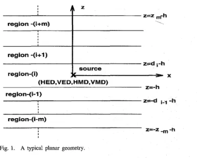
Since the main goal of this paper is to introduce a robust technique to obtain the spatial-domain Green’s functions in closed forms for planarly-layered media, Fig. 1, it would be useful to give the definition of the spatial-domain Green’s functions
where, G and G are the Green’s functions in the spatial and spectral domains, respectively,
H i 2 )
is the Hankel function of the second kind and S I P is the Sommerfeld integration path defined in Fig. 2. Note that this integral, called the Sommerfeld integral, can not be evaluated analytically for the spectral- domain Green’s functions G, which are obtained analytically for planarly stratified media [ 5 ] , [9]. It was recognized by Chow et al. [3] that if the spectral-domain Green’s function G is approximated by exponentials, the Sommerfeld inte- gral (1) can be evaluated analytically using the well-known Sommerfeld identityTherefore, this places the emphasis of deriving the closed- form Green’s functions on the exponential approximation. Since the approximation techniques used for this problem, namely the original Prony, the least square Prony and the GPOF methods, require uniform samples along a real variable of a complex-valued function, one might think of choosing the integration path in (1) along the real
IC,
axis so that G can be sampled along a real variable. However, one should notice thatk:
= IC2 -IC;
and sampling along realIC,
results in an approximation in terms of exponentials of IC, which cannot be cast into a form of exponentials ofIC,
as required in the application of the Sommerfeld identity (2). Hence, a deformed path on IC, plane, denoted by Cap in Fig. 2, was defined as a mapping of a real variable t onto the complex IC, plane byZ=Z ,-h
region -(i+m) 1
region-(i-m)
Z=-Z -m -h
Fig. 1. A typical planar geometry.
where IC, and
IC
are defined in the source layer [3]. The Green’s functions are sampled uniformly ont
E [0, T o ] , which maps onto the path Cap with ICpmax = k [ l + T2]1/2 in the IC,-plane, and approximated in terms of exponentials of t which can easily be transformed into a form of exponentials of IC,. This scheme is called the one-level approximation approach here in this paper because the complex function to be approximated is sampled between zero and To and is assumed to be negligible beyond To.For a general-purpose algorithm, the spectral-domain Green’s functions are obtained for a multilayer medium and neither surface-wave poles nor the real images are extracted. It is true that the extraction of the surface-wave poles (SWP) and the real images would have helped the exponential approximation techniques by making the Green’s functions in the spectral domain well-behaving (extraction of the SWP’s) and fast-converging (extraction of the real images). However, since the contribution of the SWP’s is small for geometries on a thin substrate, and there is no analytical way of finding the real images for multilayer planar structures except for simple cases like single and double layers, the help gained for the approximation would be limited to a restricted class of planar geometries and would render the algorithm not general purpose and not robust.
It would be instructive to consider the practical details of the implementation of the exponential approximation along the path defined in (3). It is of utmost importance to choose the approximation parameters; To, the number of exponen- tials to be used in the approximation, and the number of samples in t E [0, T o ] , judiciously for the success of this approach. To illustrate the implementation of the one-level exponential approximation and the difficulties involved, the spectral-domain Green’s function for the scalar potential due to an x-directed dipole,
Gz,
is given in Fig. 3, for a geometry of four layers at 30 GHz: First layer-PEC; second layer-E,Z = 12.5,dz = 0.03 cm; third l a ~ e r - 6 ~ 3 = 2.1,d3 = 0.07 cm; fourth layer-free-space, and the source and observation planes are chosen at the interface of the second and third layers. Since the expressions of the spectral-domain Green’s functions in a
AKSUN A ROBUST APPROACH FOR THE DERIVATION OF CLOSED-FORM GREENS FUNCTIONS 653
kp
-
planeFig. 2. Definition of the Sommerfeld integration path and the path Cap used in one-level approximation.
4.0
Imaginary
4.0
0.0 0.2 0.4 0.6 0.8 1.0
t
Fig. 3. The magnitude of the spectral-domain Green’s function G!: along the path Cap. First layer-PEC; second Iayer-e,z = 12.5, dz = 0.03 cin; third layer-e,3 = 2.1, d3 = 0.07 cm; fourth layer-free-space, freq = 30 GHz.
multilayer medium are given in [5] for HED, VED, HMD, and VMD sources, they are not included in this paper. It is evident from Fig. 3 that Green’s functions can have sharp peaks and fast changes for small t , which maps to thie far- field region in the spatial domain. Therefore, one needs to sample the Green’s function given in Fig. 3 at a peniod of less than 0.05 along
t
so that the fine features of the function can be captured in the approximation. The choice of To is another parameter that competes with the period of samples because large To corresponds to large number of samples and translates to a longer CPU time. Fortunately, for the example given in Fig. 3, the Green’s function decays quite fast in the spectral domain, therefore it would be enough to sample as far as To = 5 which requires 200 samples if A tis chosen to be 0.025. The spatial-domain Green’s function is obtained via the GPOF method using the above approximation parameters (To = 5, number of samples = 201, number of exponentials = 13) and compared to the result obtained from the numerical integration, which are labeled as “Apprx.” and “Exact,” respectively, in Fig. 4. Although, as it was mentioned above, the SWP’s are not extracted from the spectral-domain Green’s function prior to the exponential approximation, the contribution of the SWP’s is also shown for the purpose of comparison and one can draw a conclusion that the exponential approximation algorithm (GPOF) works fine well withiin the influence range of the SWP’s and beyond that an asymptotic
15.0 14.0 13.0 12.0 11.0.
-.
- Approx.-
Exact SW contribution -a
_ _ _ _ 1.0 3 -2.0 -1.0 0.0Fig. 4. The magnitude of the Green’s function for the scalar po- tential and the surface wave contribution. First layer-PEC; second layer-e,z = 12.5,dz = 0.03 cm; third layer-c,~ = 2.l,d3 = 0.07 cm; fourth layer-free-space, freq = 30 GHz.
approximation together with the surface-wave contribution can be used to approximate the spatiad-domain Green’s functions [1C% [ I l l .
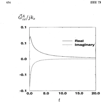
lJnfortunately, not all the Green’s functions have fast de- caying spectral-domain behavior like the above example given in Fig. 3. For example, the spectral-domain Green’s function for the vertical component of the vector potential due to a 13ED [5], G&./jkz = Gfy/jky, does not decay as fast
and moreover has a relatively isharp peak which requires sampling almost as frequently as that of the example given in Fig. 3, as shown in Fig. 5. To demonstrate the effect of the approximation parameters, the Green’s function J Gf, dx (=
~ - - ~ { G t . / j k ~ } ) is given for thie same approximation pa- rameters as those of the above (example (To = 5, number of samples = 201) and compared to the results obtained by the numerical integration of the spectral-domain representation of the Green’s function and to thte results obtained by using different approximation parameters in Fig. 6. It is observed that the approximated Green’s fiinctions do not agree with the exact solution for small values of p because the spectral- doinain Green’s function is not sampled far enough to get an accurate near-field distribution. However, if the value of
654 E E E TRANSACTIONS ON MICROWAVE THEORY AND TECHNIQUES, VOL. 44, NO. 5, MAY 1996 0.1 Real lmaglnary ... ... 0.0 - ... I -0.1 -0.1
’
0.0 5.0 10.0 15.0 21t
Fig. 5. The magnitude of the spectral-domain Green’s function G& /jkz. First layer-PEC; second layer-e,:! = 12.5,dz = 0.03 cm; third layer-t,3 = 2.1, d3 = 0.07 cm; fourth layer-free-space, freq = 30 GHz.
exact Green’s functions is improved at the expense of the computation time provided that the frequency of sampling is kept constant.
From the above discussion, it can easily be concluded that the one-level approximation approach can not be made fully robust and suitable for the development of C A D software. As it was mentioned above, this is because it requires users first to investigate the spectral-domain behavior of the Green’s function and then to perform a few iterations to find the best possible combination of the approximation parameters. To circumvent these difficulties, a two-level approximation scheme is developed here in conjunction with the use of the GPOF method and its details are given in the following section. 111. TWO-LEVEL APPROACH FOR APPROXIMATING
THE SPECTRAL-DOMAIN GREEN’S FUNCTIONS
To alleviate the necessity of investigating the spectral- domain Green’s functions in advance and the difficulties caused by the trade-off between the sampling range To and the
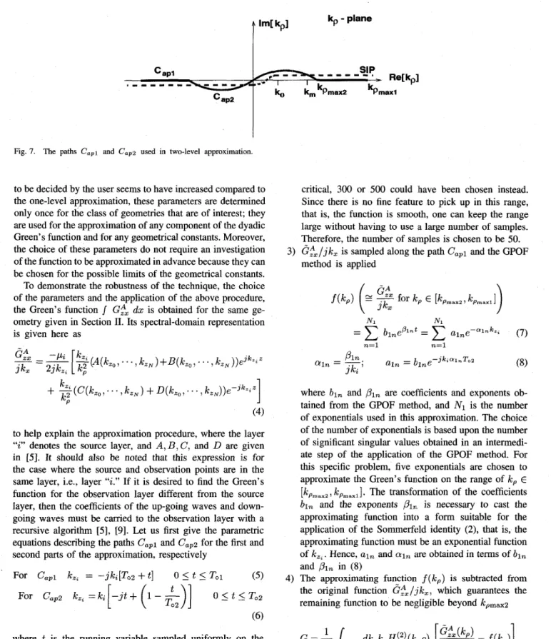
sampling period, the approximation is performed in two levels. The first part of the approximation is performed along the path
Capl while the second part is done along the path Cap2, as shown in Fig. 7. Note that the second part of the approximation is the same as the one-level approximation scheme described in the previous section, except that now the value of Toz
(kpmaxz = k [ l
+
T22]1/2) can be set in advance to a value such that kpmaxz 2 k , where k , is the maximum value of the wavenumber involved in the geometry.To illustrate the procedure of the two-level approximation, we will first outline the necessary steps and then provide some of the details. The steps are:
1) Choose T02 such that ICPmaxZ 2 k , : For exam- ple, since GaAs is the highest dielectric constant layer (E,(GaAs) = 12.5), then IC, = m k , , and T02 can be safely chosen to be five.
-8.0 -8.5 -9.0 -9.5 0 ~ Exact - 0 x - Apprx.( T0=5, # of sample=20l) El Apprx.(TO=lO, # of sample=401) x Apprx.(TO=50, # of sample=601) -1 0.0 -3.0 -2.0 -1 -0 0.0 1.0
Fig. 6. The magnitude of the Green’s function for the vector potential G& dx. First layer-PEC; second layer-€,:! = 12.5, d:! = 0.03 cm; third layer-e,3 = 2.1, d3 = 0.07 cm; fourth layer-free-space, freq = 30 GHz.
2 ) Choose Tol, i.e.,
ICPmax1
= k [ l+
(Tol+
To2)2]1/2, and the number of samples on [kPmaxz,ICPmaxl]:
The choice of To, is not very critical as long as one choosesICPmax1
large enough to pick up the behavior of the spectral- domain Green’s function for large IC,, and, since thespectral-domain behaviors of the Green’s functions are always smooth beyond ICPmax2, it is not necessary to have a large number of samples on
[kPmauZ,
ICPmaxl].
Typical values could be 200 for Tol and 200 for the number of samples.3) Sample the function along the path Capl and approxi-
mate it by using the GPOF method: Sampling along the path Capl can be performed by varying t between zero
and TOl uniformly in k , = -jIC[T02
+
t].4) Subtract the function approximated for the range of
ICP E
[kpmaxz,
ICpmaxl] from the original function: The remaining function will be nonzero over a small range ofk,
(E [O,kPmaxz]) so that one can pick up the fine features of this function without employing a huge number of sampling points.5) Sample the remaining function uniformly along the path
Ca,z and approximate it by using the GPOF method: Sampling along the path Cap, can be performed by varying t between zero and T02 uniformly in IC, = The parameters that must be fixed by the user in advance are the limits of the sampling ranges Tol and T02 for the first
and the second parts of the approximation, respectively, and the number of samples along the paths CaP1 and Caps, which respectively correspond to the first and second parts of the approximation. Although the number of parameters which are
AKSUN: A ROBUST APPROACH FOR THE DERIVATION OF CLOSED-FORM GREEN‘S FUNCTIONS 655
t
ImLkplkp
-
planeCap2
Fig. 7. The paths C,,l and Capz used in two-level approximation.
to be decided by the user seems to have increased compared to the one-level approximation, these parameters are determined only once for the class of geometries that are of interest; they are used for the approximation of any component of the dyadic Green’s function and for any geometrical constants. Moreover, the choice of these parameters do not require an investigation of the function to be approximated in advance because they can be chosen for the possible limits of the geometrical constants. To demonstrate the robustness of the technique, the choice of the parameters and the application of the above procedure, the Green’s function J Gtx dx is obtained for the same ge- ometry given in Section 11. Its spectral-domain representation is given here as
to help explain the approximation procedure, where the layer
“i” denotes the source layer, and A, B, C, and D are given in [5]. It should also be noted that this expression is for the case where the source and observation points are in the same layer, i.e., layer “i.” If it is desired to find the Green’s function for the observation layer different from the source layer, then the coefficients of the up-going waves and clown- going waves must be carried to the observation layer with a recursive algorithm [5], [9]. Let us first give the parametric equations describing the paths C,,l and Cap2 for the first and
second parts of the approximation, respectively
. For Cap1 ICzs = -jICi[T02
+
t] 05
t5
To1 ( 5 )For Cap, ICz, =kc;
[
- j t +(
1 --
;2)] 0 5 t 5 T o 2where t is the running variable sampled uniformly on the corresponding range. Then, the above procedure is followed step-by-step as:
1) T02 = 5 is chosen, for which ICfmaxz = k i [ l
+
To2]1/2
>
,1 =Lo.
2) = 400 is chosen to ensure that the behavior of Gfx/jIC, for large 1, is captured. This choice is not
3)
4)
critical, 300 or 500 could have been chosen instead. Since there is no fine feature to pick up in this range, that is, the function is smooth, one can keep the range large without having to use a large number of samples. Therefore, the number of samples is chosen to be 50.
G:x/jICx is sampled along the path Cap, and the GPOF
method is applied
Ni Ni
n=l n = l
where bl, and Pln are coefficients and exponents ob- tained from the GPOF methlod, and Nl is the number of exponentials used in this approximation. The choice of the number of exponentials is based upon the number of significant singular values obtained in an intermedi- ate step of the application of the GPOF method. For this specific problem, five axponentials are chosen to approximate the Green’s function on the range of IC, E
[ICpmaxz, ICpmaxl]. The transformation of the coefficients
bln and the exponents
Pln
is necessary to cast the approximating function into a form suitable for the application of the Sommerfeld identity (2), that is, theapproximating function must be an exponential function of k z * . Hence, aln and a1, are obtained in terms of b l ,
The approximating function f ( k p ) is subtracted from the original function
GtX/;iIC,,
which guarantees the remaining function to be negligible beyond ICpmax2and Pln in (8)
dICpk,H~2)(k,p)
[
-
f ( k , ) ]Note that the first integral is evaluated along the path
656 JEEE TRANSACTIONS ON MICROWAVE THEORY AND “ I Q U E S , VOL. 44, NO. 5 , MAY 1996 Exact Apprx. (two-level) Apprx. (one-level) -10.0
’
I -3.0 -2.0 -1.0 0.0 1.01 og10
(IC0 P ) Fig. 8.layer-e,3 = 2.1, d3 = 0.07 cm; fourth layer-free-space, freq = 30 GHz. The magnitude of the Green’s function for the vector potential G:= dx. First layer-PEC; second layer-e,z = 12.5, dz = 0.03 cm; third
the second integral is evaluated along Cup2
+
CUp1.Therefore, the Sommerfeld identity (2) can be applied to the integrals in (9).
5) The remaining function is sampled along the path Cu,2 with 100 samples. Since the maximum range for the sampling ( k p m a x 2 ) is rather small, compared to that of the one-level approximation scheme, the frequency of sampling can be made quite high without substantially increasing the number of samples. For all practical purposes (including the worst case situation) the choice of 200 as the number of samples would be more than enough to get a good approximation
where b2, and t32n are the coefficients and exponents of the exponentials of
t
obtained from the application of the GPOF method, and and azn are the coefficientsand exponents of the exponentials of kzt. The number
of exponentials N2 in this part of the approximation is chosen to be 8, again by the number of significant singular values.
To summarize, the approximation parameters as chosen here are as follows: for the first part of the approximation;
TOl = 400, To2 = 5, number of samples = 50, and number of
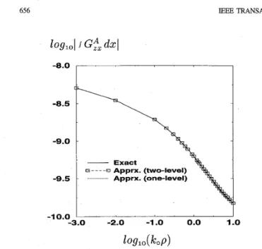
exponentials = 5, for the second part of the approximation; number of samples = 100, number of exponentials = 8. Note that the total number of exponentials used in this approxi- mation is 13. The Green’s function obtained by employing the above procedure is given in Fig. 8 along with the data obtained from direct numerical evaluation of the Sommerfeld-
4.0 0 Apprx.(GAxx 2.0 0.0 -2.0 1.0 -3.0 -2.0 -1.0 0.0 oil10 ( L O P
1
0 Apprx. (GAzz) 0 Apprx. (Gqz) - ExacttGqz) -3.0 -2.0 -1.0 0.0 1 .o (b)Fig. 9. (a) The magnitude of the normalized Green’s functions 4aG&,/p3,4ae3GZ. First layer-PEC; second layer-c,z = 12.5,dz = 0.03 cm; third layer-e,s = 2.l,d3 = 0.07 cm; fourth layer-free-space, freq = 30 GHz. (b) The magnitude of the
normalized Green’s functions 4nGtz,/p3, 4ne3G;. First layer-PEC; second layer-e,Z = 12.5,dz = 0.03 cm; third layer-e,3 = 2.1, ds = 0.07 cm; fourth layer-freespace, freq = 30 GHz.
type integral (exact), and from the one-level approximation approach with the parameters of approximation To = 200, number of samples = 400 and the number of exponentials = 13. Note that the values of the parameters used in the one-level approximation are chosen to make the computation time minimum with a reasonable agreement. However, those of the two-level approximation are typical values and the number of samples for the second part of the approximation can even be reduced to 50 with no change in the results. The two approximation techniques for the above example are compared for the CPU time on a SPARCstation 10/41, using
AKSUN: A ROBUST APPROACH FOR THE DERIVATION OF CLOSED-FORM GREEN’S FUNCTIONS 651 0.0 -2.0 -4.0 -6.0 4.0
:--,-
-e.-&---__
. ..._, 4. -.-. .-..__ m....-. 2.0 - - 0 Exact <I=lGHzl %L - - - Apprx. (f-lGHz) n Exaci (f-rlOGNz) Apprx. (f=loOHz) 0 Exact (f-lOOGHz) _ _ _ _ Apprx. (t=lOOGHz) .10.0 -8-o -3.0-
-2.0 -1.0 0.0 1 .o l O 9 l O ( k O P> (a) 4.0 2.0 0.0 -6.0’
. ’ I -3.0 -2.0 -1.0 0.0 1 .o (b)Fig. 10. (a) The magnitude of the normalized Green’s function 47rG&/p3.
First layer-PEC; second layer-e,z = 12.5,dz = 0.03 cm; third layer-e,3 = 2.l,d3 = 0.07 cm; fourth layer-free-space. (b) The magnitude of the normalized Green’s function 4ae3Gg. First layer-PEC; second layer-e,z = 12.5,dz = 0.03 cm; third layer-e,3 = 2.1, d3 = 0.07 cm; fourth layer-free-space.
the same number of total exponentials (= 13) for different approximation parameters, and presented in the table format below:
Approximation CPU time
Approximation Parameters (set)
one-level
To
= 200, N, = 400 198.0 one-level To = 200, N , = 500 382.0 two-level two-levelTOl
= 400, N,, = 50Tol
= 400, N,, = 50 Toz = 5 , N,, = 50T02
= 5, N,, = 100 1.2 3.5where N , is the number of samples in one-level approximation scheine while Nsl and Ns2 are the number of samples of the first and second parts of the approximation, respectively, in the two-level approximation approach. It is obvious that the two- level approximation approach improves the computational efficiency significantly.
The robustness of the two-level approach can be demon- strated by casting the other Green’s functions into closed forms with the use of the same approximation parameters as those: used for
1
G&dx,
namelyT0l
= 400,N,, = 50 To2 := 5 , N,, = 100. The normalized Green’s functions of the vector and scalar potentials due to HED and VED sources are obtained (47rG&/p3,47r~G$, 47rGfZ/p3 and 4m3G9 following the two-level approach (Apprx.) and evaluating the !$ommerfeld integrals numerically (Exact), and given in Fig. 9(a) and (b). This test shows thlat the same set of approx- imat,ion parameters can be used for any Green’s function, that is, there is no need for an advance investigation of the Green’s function and no need for any trial steps. The assessment of the robustness of the proposed approach also requires a stud!{ of the sensitivity of the approximation parameters to the geometrical constants and the frequency. Therefore, the Green’s functions for the vector and the scalar potentials are o b t a “ in closed forms for the same geometrical constants and for the same approximation piirameters used above, but the frequency of operation is changed to 1 GHz, 10 GHz and 100 GHz, which is equivalent, in effect, to a change of the geometrical constants, Fig. 10(a) and (b). It is observed that the agreements between the exact and approximate sets of data are still perfect and hence it is safe to conclude that the two-level approach proposed in this paper is very robust.IV. CONCLUSION
The closed-form Green’s functions developed previously suffer from the difficulties of choosing approximation param- eters, for the exponential approximation techniques used in the derivation, thereby rendering the technique to be inefficient and not robust. Moreover, the extraction of the SWP’s and real images may not be possible or efficient for multilayer geornetries when the original approach is used. Here, a new approach based on a two-level approximation is proposed to overcome these difficulties and to make the use of closed-form Green’s functions attractive for those developing EM software and for researchers in the field. The major advantages of this approach are its robustness and the: computational efficiency, both of which are demonstrated in the text.
REFERENCIES
[ l ] R. F. Harrington, Field Computation by Moment Methods. Malabar,
n:
Krieger, 1983.[2] A. Taflove, “State of the art and future directions in finite-difference and related techniques in supercomputing computational electromagnetics,” in Directions in Electromagnetic Wave’ Modeling, H. L. Bertoni, and L. B. Felsen, Eds. New York Plenum, 1991.
[3] Y. L. Chow, J. J. Yang, D. F. Fang, and G. E. Howard, “A closed-form spatial Green’s function for the thick microstrip substrate,” IEEE Trans. Microwave Theory Tech., vol. 39, pp. 588-592, Mar. 1991.
[4] M. I. Aksun and R. Mittra, “Derivation of closed-form Green’s functions for a general microstrip geometries,” IEEE Trans. Microwave Theory Tech., vol. 40, pp. 2055-2062, Nov. 1992.
658 IEEE TRANSACTIONS ON MICROWAVE THEORY AND TECHNIQUES, VOL. 44, NO. 5, MAY 1996 [51 [71 [81 [91 I101
G . Dural and M. I. Aksun, “Closed-form Green’s functions for general sources and stratified media,” IEEE Trans. Microwave Theory Tech., vol. 43, pp. 1545-1552, July 1995.
A. J. Mackay and A. McCowan, “An improved pencil-of-function method for extracting poles of an EM system from its transient re- sponse,” IEEE Trans. Antennas Propagat., vol. AP-35, pp. 4 3 5 4 1 ,
Apr. 1987.
D. G. Dudley, “Parametric modeling of transient electromagnetic sys- tems,’’ Radio Sci.,, vol. 14, pp. 387-396, 1979.
Y. Hua and T. K. Sarkar, “Generalized pencil-of-function method for extracting poles of an EM system from its transient response,” IEEE
Trans. Antennas Propagat., vol. AP-37, pp. 229-234, Feb., 1989.
W. C. Chew, Waves and Fields in Inhomogeneous Media. New York Van Nostrand, 1990.
Sina Barkeshli, P. H. Path& and Miguel Marin, “An asymptotic closed- form microstriu surface Green’s function for the efficient moment method analysis of mutual coupling in microstrip antennas,” IEEE Trans.
Antennas Propagat., vol. 38, pp. 1374-1383, Sept. 1990.
[ l l ] L. B. Felsen and N. Marcuvitz, Radiation and Scattering of Waves. Englewood Cliffs, NJ: Prentice-Hall, 1973.
M. I. Aksun (M’92) received the B.S. and M.S. degrees in electrical and electronics engineenng from the Middle East Technical University, Ankara, Turkey, in 1981 and 1983, respectively, and the Ph.D. degree in electrical and computer engineering from the University of Illinois at Urbana-Champaign in 1990.
From 1990 to 1992, he was a post doctoral fellow at the Electromagnetic Communication Laboratory, University of Illinois at Urbana-Champaign. Since 1992, he has been on the faculty of the Department of Electrical and Electronics Engineering at Bilkent University, Ankara, Turkey, where he is currently an Associate Professor. His research interests include the numerical methods for electromagnetics, microstrip antennas, and microwave and millimeter-wave integrated circuits.