Image classification using subgraph histogram representation

(1)

Image Classification Using Subgraph Histogram Representation

Bahadır ¨Ozdemir, Selim Aksoy Department of Computer Engineering

Bilkent University Bilkent, 06800, Ankara, Turkey {bozdemir,saksoy}@cs.bilkent.edu.tr

Abstract—We describe an image representation that com-bines the representational power of graphs with the efficiency of the bag-of-words model. For each image in a data set, first, a graph is constructed from local patches of interest regions and their spatial arrangements. Then, each graph is represented with a histogram of subgraphs selected using a frequent subgraph mining algorithm in the whole data. Using the subgraphs as the visual words of the bag-of-words model and transforming of the graphs into a vector space using this model enables statistical classification of images using support vector machines. Experiments using images cut from a large satellite scene show the effectiveness of the proposed representation in classification of complex types of scenes into eight high-level semantic classes.

I. INTRODUCTION

Histogram of visual words obtained using a codebook constructed by quantizing local image patches has been a very popular representation for image classification in the recent years. This representation, also called the bag-of-words model [1], has been shown to give successful results for different image sets. However, a commonly accepted drawback is its disregarding of the spatial relationships among the individual patches as these relationships become crucial as contextual information for the understanding of complex scenes.

As another extreme, graph-based representations provide powerful structural models [2], [3] where the nodes can store local content and the edges can encode spatial information. However, their use for image classification has been limited due to difficulties of translating the complex image content to graph representations and inefficiencies in comparisons of these graphs for classification. For example, the graph edit distance works well for matching relatively small graphs [4] but it can become quite restrictive for very detailed image content with a large number of nodes and edges such as the graphs constructed for satellite images [5].

This paper proposes an intermediate representation that combines the representational power of graphs with the efficiency of the bag-of-words representation. We describe a method for transforming the scene content and the asso-ciated spatial information of that scene into graph data. The proposed approach represents each graph with a histogram of frequent subgraphs where the subgraphs encode the local patches and their spatial arrangements. First, local patches of

interest are detected using maximally stable extremal regions obtained by gray level thresholding. Next, these patches are quantized to form a codebook of local information, and a graph for each image is constructed by representing these patches as the graph nodes and connecting them with edges obtained using Voronoi tessellations. Then, these graphs are approximated with histograms of subgraphs. The subgraphs that are used as the visual words of the final bag-of-words model are selected using a frequent subgraph mining algorithm. The frequent subgraphs are used to avoid the need of identifying a fixed arbitrary complexity (in terms of the number of nodes) and to require that they have a certain amount of support in different images in the data set. Consequently, the spatial structure in the image is encoded in a histogram, and the graph matching problem is transformed into a vector space that reduces the computational cost. We show that good results for classification of images cut from large satellite scenes can be obtained for eight high-level semantic classes using support vector machines together with feature selection.

The rest of the paper is organized as follows. Section II describes the graph representation for an image. Sec-tion III introduces the subgraph histogram representaSec-tion. Section IV presents the procedure for image classification. Performance evaluation using an Ikonos image of Antalya, Turkey is given in Section V, and Section VI provides the conclusions.

II. GRAPH REPRESENTATION A. Detection of image patches

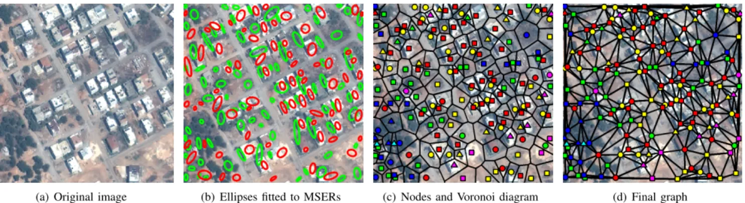
The input to the proposed method consists of satellite images with both panchromatic (gray level) and multi-spectral (RGB) bands. To find regions of interest in such an image, we use the maximally stable extremal region (MSER) method which selects highly stable regions from all possible thresholdings of a gray level image [6]. The method is applied to the original gray level input image (MSER+) and its inverted image (MSER-). An ellipse is fitted to each MSER. The MSER+ and MSER- ellipses for the image in Figure 1(a) are shown as green and red, respectively, in Figure 1(b). The resulting MSERs enable modeling of local image content without the need for a 2010 International Conference on Pattern Recognition

1116

2010 International Conference on Pattern Recognition

1116

1112

(2)

(a) Original image (b) Ellipses fitted to MSERs (c) Nodes and Voronoi diagram (d) Final graph

Figure 1. Feature extraction and graph construction steps. MSER+ and MSER- ellipses are shown as green and red, respectively, in (b). The color and symbol of a node in (c) and (d) represent its label after k-means clustering.

precise segmentation that can be quite hard for such high spatial resolution satellite images.

The next step is to extract features from these MSERs. To make regions more discriminative, the ellipses are ex-panded by a scale factor, and the pixels inside the ellipses are divided into two groups representing the stable region and its surroundings according to their relative distances to the ellipse center. From the panchromatic band, mean and standard deviation, and from the RGB bands only the mean values are computed for both groups of pixels. We also compute morphological granulometry features from the panchromatic band using opening and closing with disk structuring elements with radii of two and seven pixels. Moment of inertia, size, and aspect ratio of the ellipses are other features extracted from these patches. The resulting 17 rotation-invariant features are normalized to zero mean and unit variance separately for MSER+ and MSER-.

B. Graph construction

The spatial relationships between MSERs can be exploited by constructing a graph from these regions. The centers of ellipses fitted to MSERs form the graph nodes, and their labels are determined from k-means clustering of the extracted features. The final step of graph construction is to connect every neighbor node pair with an edge. We can determine whether given two nodes are neighbors or not by computing the Euclidean distance between the centroids of the nodes and comparing it to a threshold. However, such a threshold is scale dependent and cannot be automatically set for different scenes. In addition, a global threshold defined for all scene types creates more complex graphs for the images where the number of nodes is high like urban areas and it may produce unconnected nodes for the images with fewer number of nodes such as fields.

To handle these problems we use the Voronoi tessellation where the nodes correspond to cell centroids. The nodes whose cells are neighbors in the Voronoi tessellation are considered as neighbor nodes and are connected by undi-rected edges. For the image in Figure 1(a), the nodes and

the corresponding Voronoi diagram are shown in Figure 1(c). The color and symbol of a node represent its label. The final graph of the image can be seen in Figure 1(d).

III. SUBGRAPH HISTOGRAM REPRESENTATION A. Frequent subgraph mining

As discussed earlier, subgraphs can provide useful infor-mation about the image content because they capture struc-tural information. We consider only the frequent subgraphs in this study because enumerating all possible subgraphs is often not feasible, but subgraphs with different degrees can be considered and a subset can be selected instead of fixing the degree while also guaranteeing a reasonable support in multiple images in the data set. Using a subset of possible subgraphs also avoids the curse of dimensionality in the final histogram representation.

The graph mining literature includes several approaches for frequent subgraph mining. According to [7], frequent subgraph mining is to find every graph, g, whose support in a graph set, GS = {Gi|i = 1, . . . , N }, is equal or greater than

a threshold, minSup. The support of g in GS is denoted as σ(g, GS), and is generally defined as the number of graphs in GS that have a subgraph which is isomorphic to g.

In our application, the number of times a subgraph occurs in an image graph provides more information than the binary information about whether the image graph contains the subgraph or not. Therefore, we use another support measure instead of the traditional one. An embedding (subgraph isomorphism) is defined as a mapping from a subgraph, g, to an input graph G where the labels of corresponding nodes and edges have to be the same for every node and edge of g. Two different embeddings may refer to the same nodes or edges as in Figure 2. There are seven embeddings of the subgraph into the input graph where every embedding refers to at least one node which is also referred by another one.

Kuramochi and Karypis [8] introduced maximum inde-pendent set (MIS) support for handling overlapping sub-graphs. The idea is based on finding the maximum number

1117 1117 1113 1113 1113

(3)

(a) Input graph (b) Subgraph Figure 2. An example for overlapping subgraphs.

(a) Input graph (b) Subgraph

Figure 3. Another example for overlapping subgraphs.

of embeddings which do not have any overlapping node. According to this definition, MIS-support of the subgraph in Figure 2 is only two. However, MIS-support is sometimes too restrictive about overlaps, so a new support definition, harmful overlap (HO) support, is introduced by Fiedler and Borgelt [9]. According to this definition, the overlap in Figure 3 is not considered as a harmful overlap because neither of the white nodes in the subgraph are not mapped to the same node in both embeddings. The HO-support of the subgraph in Figure 3 is computed as two while the MIS-support is only one. To determine whether two embeddings overlap harmfully or not, the method examines ancestor embeddings where the details can be found in [9]. The graph set in our application includes many overlapping embeddings so we use the HO-support for the function σ(g, G) in order to handle overlapping subgraphs more accurately.

In our data set, the numbers of images in different classes are not equal and the number of nodes in an image varies according to its class. In addition, the frequency of some subgraphs is particularly high in some classes. Therefore, we use different support thresholds selected empirically for each class instead of a global threshold, and the sets of frequent subgraphs are found using the graph sets of training images for each class independently. Finally, these sets of frequent subgraphs are combined into a single set S.

B. Histogram feature vector

The subgraph histogram provides a powerful represen-tation that is not as complex as full graph models, and reduces the complexity of graph similarity computation. The histogram is constructed using the support of each subgraph in S. Each image graph G in the data set GS is transformed into a histogram feature vector

x = (x1, . . . , xn) (1)

where xi = σ(gi, G) and gi ∈ S for i = 1, . . . , M .

Consequently, images can be classified in this feature space using statistical pattern recognition techniques.

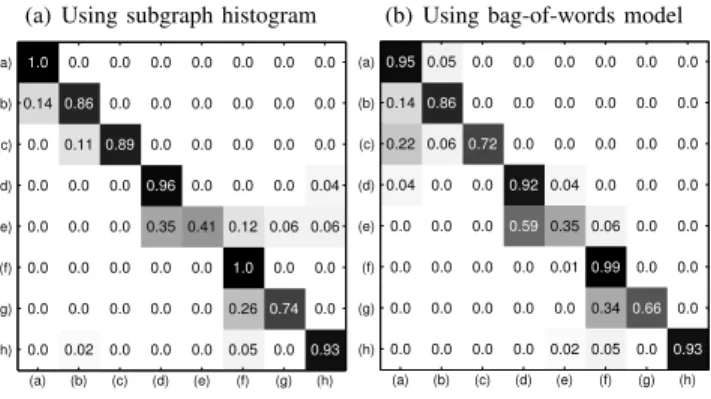
Table I

CONFUSION MATRICES. CLASS NAMES ARE GIVEN IN THE TEXT. (a) Using subgraph histogram (b) Using bag-of-words model

IV. IMAGE CLASSIFICATION

The set of all frequent subgraphs, S, may not be dis-criminative enough for classification, and many subgraphs in S may also share some redundant fragments. Hence, postprocessing is required for selecting the most valuable subgraphs in S to also avoid redundancy that leads to the curse of dimensionality. We use the sequential forward selection algorithm to find a subset S∗ which includes the most valuable subgraphs.

We use a multi-class support vector machine (SVM) with a radial basis function kernel for classification. The multi-class SVM is a combination of one-against-one class SVMs where the output class is the one with the maximum number of votes. The subgraphs used in the classifier are incrementally selected using the forward selection algorithm with the correct classification accuracy for the training data as the quality measure.

V. EXPERIMENTS

The experiments were performed on a 14204 × 12511 pixel Ikonos image of Antalya, Turkey, consisting of a panchromatic band with 1 m spatial resolution and four multi-spectral bands with 4 m spatial resolution. We use this image because of its diverse content including several types of complex high-level structures such as dense and sparse residential areas with large and small buildings as well as fields and forests. The whole image was partitioned into 250 × 250 pixel tiles. Totally 585 images were used in the experiments, one half for training and the other half for testing. These images were grouped in eight classes, namely, (a) dense residential areas with large buildings, (b) dense residential areas with small buildings, (c) dense residential areas with trees, (d) sparse residential areas, (e) greenhouses, (f) orchards, (g) forests, and (h) fields.

The confusion matrices for the test data are shown in Table I, and example images from the classification results are shown in Figure 4. Some parameters have a major effect on the performance. Large number of patch clusters

1118 1118 1114 1114 1114

(4)

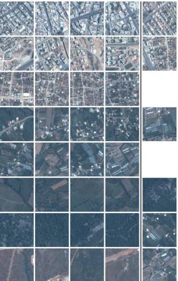
Figure 4. Example images for each class. Images in the first four columns are correctly classified where the ones in the last column are misclassified. The rows correspond to the rows of the confusion matrix.

reduces the occurrence frequency of subgraphs. As a result, finding a subgraph of S in the testing set becomes harder. A similar effect is observed when the minimal degree of subgraphs in S is large. On the other hand, smaller number of cluster patches and subgraphs with one or two nodes are not sufficient to distinguish two image graphs from similar classes, for example forests and orchards. In the experiments, the MSERs are grouped into 30 clusters using the k-means algorithm. For each class approximately the top 100 frequent subgraphs are combined in the set S. The size of S∗ is determined as 30 in order to compare our method with a traditional bag-of-words model in the same dimensionality where the individual clustered MSERs are used as the words. As seen in the confusion matrices in Table I, the accuracy is improved by the subgraph histogram representation in comparison to the bag-of-words model. For both cases,

greenhouses (e) is the most confused class. In our Ikonos image, greenhouses are located near the sparse residential areas (d) and orchards (f). Therefore, the images of green-houses are not homogeneous and contain structures belong-ing to other classes. In addition, some small confusions are observed between similar classes, for example (a) and (b).

VI. CONCLUSIONS

We described a new image content representation using frequent subgraph histograms for classifying complex scenes such as dense and sparse urban areas. We also described a method for constructing an image graph which encapsulates the spatial information of the scene. In the proposed method, recurring spatial structures of a scene class are encoded in a histogram of frequent subgraphs. Finally, we use a multi-class SVM together with subgraph selection in order to classify the image graphs. Image classification experiments using Ikonos images showed that the proposed model im-proves the performance of the bag-of-words model using the spatial information encoded in the subgraph histogram representation.

ACKNOWLEDGMENT

This work was supported in part by the TUBITAK CA-REER Grant 104E074.

REFERENCES

[1] L. Fei-Fei and P. Perona, “A Bayesian hierarchical model for learning natural scene categories,” in CVPR, 2005, pp. 524– 531.

[2] H. Bunke, “Graph matching: Theoretical foundations, al-gorithms, and applications,” in Vision Interface, Montreal, Canada, May 14–17, 2000.

[3] D. Conte, P. Foggia, C. Sansone, and M. Vento, “Thirty years of graph matching in pattern recognition,” International Jour-nal of Pattern Recognition and Artificial Intelligence, vol. 18, no. 3, pp. 265–298, May 2004.

[4] K. Riesen and H. Bunke, “IAM graph database repository for graph based pattern recognition and machine learning,” in S+SSPR, 2008, pp. 287–297.

[5] S. Aksoy, “Modeling of remote sensing image content using attributed relational graphs,” in S+SSPR, 2006, pp. 475–483. [6] J. Matas, O. Chum, M. Urban, and T. Pajdla, “Robust wide

baseline stereo from maximally stable extremal regions,” in BMVC, 2002, pp. 384–393.

[7] X. Yan and J. Han, “gSpan: Graph-based substructure pattern mining,” in ICDM, 2002.

[8] M. Kuramochi and G. Karypis, “Finding frequent patterns in a large sparse graph,” Data Min. Knowl. Discov., vol. 11, no. 3, pp. 243–271, 2005.

[9] M. Fiedler and C. Borgelt, “Support computation for mining frequent subgraphs in a single graph,” in MLG, 2007.

1119 1119 1115 1115 1115