LOW POWER RANGE ESTIMATION WITH
DSSS TECHNIQUE IN UNDERWATER
ACOUSTICS
a thesis
submitted to the department of electrical and
electronics engineering
and the graduate school of engineering and science
of bilkent university
in partial fulfillment of the requirements
for the degree of
master of science
By
Mustafa Ozan G¨
ulery¨
uz
I certify that I have read this thesis and that in my opinion it is fully adequate, in scope and in quality, as a thesis for the degree of Master of Science.
Prof. Dr. Hayrettin K¨oymen(Advisor)
I certify that I have read this thesis and that in my opinion it is fully adequate, in scope and in quality, as a thesis for the degree of Master of Science.
Prof. Dr. Yusuf Ziya ˙Ider
I certify that I have read this thesis and that in my opinion it is fully adequate, in scope and in quality, as a thesis for the degree of Master of Science.
Assist. Prof. Dr. Satılmı¸s Top¸cu
Approved for the Graduate School of Engineering and Science:
ABSTRACT
LOW POWER RANGE ESTIMATION WITH DSSS
TECHNIQUE IN UNDERWATER ACOUSTICS
Mustafa Ozan G¨ulery¨uz
M.S. in Electrical and Electronics Engineering Supervisor: Prof. Dr. Hayrettin K¨oymen
August, 2013
Performance of direct sequence spread spectrum modulation (DSSS) in underwa-ter acoustical range finding is investigated in this thesis. Range estimation using low power DSSS codes is both analyzed theoretically and implemented at 400 kHz for experimental assessment, where the chip duration is 20 µs and sequence type is maximal. The effect of sequence length on the required transmit power is measured for sequence lengths from 7 chips to 127 chips. The performance of this method is compared to the widely used tone burst pulse range estimation technique. It is found that at a sequence of 127 chips and a pulse sequence length of 2,54 ms, range is estimated with 1,5 cm resolution using source level of 132,8 dB re 1 µP arms @ 1 m source level , while it is 190,5 cm for the same length and
magnitude tone burst modulation, at a reference test range of 4.5 m. Moreover, spectral height of received DSSS signal is well below the ambient noise level so that signal to noise ratio (SNR) for received DSSS signal is -14,8 dB, while it is 12,2 dB for received tone burst pulse
Keywords: Echo Sounding, Direct Sequence Spread Spectrum, Modulation, Range Estimation, Tone Burst Pulse.
¨
OZET
SU ALTI AKUST˙I ˘
G˙INDE DO ˘
GRUDAN D˙IZ˙IL˙I YAYILI
˙IZGE TEKN˙I ˘
G˙IN˙I KULLANARAK D ¨
US
¸ ¨
UK G ¨
UC
¸ ˙ILE
MESAFE ¨
OLC
¸ ¨
UM ¨
U
Mustafa Ozan G¨ulery¨uz
Elektrik ve Elektronik M¨uhendisli˘gi, Y¨uksek Lisans Tez Y¨oneticisi: Prof. Dr. Hayrettin K¨oymen
A˘gustos, 2013
Bu tezde do˘grudan dizili yayılı izge mod¨ulasyon (DDY˙I) y¨onteminin su altı akusti˘gi mesafe ¨ol¸c¨um¨u konusunda sergileyece˘gi ba¸sarım incelenmektedir. D¨u¸s¨uk g¨u¸cl¨u DDY˙I kodlarını kullanarak yapılan mesafe ¨ol¸c¨um¨u hem teorik a¸cıdan, hem de 400 kHz merkez frekansı kullanarak deneysel a¸cıdan tahlil edilmekte olup kullanılan ¸cip s¨uresi 20 µs, ¸cip t¨ur¨u ise maksimaldir. Dizi uzunlu˘gunun gerekli iletim g¨uc¨une etkisi 7 ¸cip dizi uzunlu˘gundan 127 ¸cip dizi uzunlu˘guna kadar ¨ol¸c¨ulmektedir. Bu y¨ontemin ba¸sarımı yaygınca kullanılan tek ton dar-beler ile mesafe ¨ol¸c¨um¨u tekni˘gi ile kar¸sıla¸stırılmaktadır. 127 ¸cip 2,54 ms uzunlu˘gunda ve 132,8 dB re 1 µP arms @ 1 m kaynak seviyesinde, DDY˙I darbesi
kulanıldı˘gında, 4.5 m’lik bir test mesafesi 1,5 cm derinlik ¸c¨oz¨un¨url¨u˘g¨u ile, aynı uzunlukta ve b¨uy¨ukl¨ukte tek ton darbe kullanıldı˘gında ise 190,5 cm ¸c¨oz¨un¨url¨uk ile ¨ol¸c¨ulmektedir. Ayrıca, DDY˙I alma¸c i¸saretinin izgesel y¨uksekli˘ginin ortam g¨ur¨ult¨us¨un¨un bir hayli altında kaldı˘gı g¨or¨ulmekte olup i¸saret g¨ur¨ult¨u oranı -14,8 dB bulunmakta, di˘ger yandan bu oran tek ton alma¸c darbesi i¸cin ise 12,2 dB olmaktadır.
Acknowledgement
I offer my sincerest gratitude to my advisor, Prof. Dr. Hayrettin K¨oymen for his support and valuable guidance.
I would like to thank to ASELSAN Inc. for encouragements and resources that are provided throughout this thesis.
I really appreciate the love and support of all my family members.
Last but not the least; I would like to express my special thanks to Ay¸seg¨ul for her endless love and patient.
Contents
1 Introduction 1
2 DSSS Ping Technology and Echo Sounding 4
2.1 Echo Sounding . . . 4
2.2 Matched Filter Concept . . . 5
2.3 Range Resolution Concept . . . 7
2.4 DSSS Modulation . . . 15
2.4.1 Important Parameters of DSSS . . . 15
2.4.2 Format of DSSS Transmitted Pulse . . . 16
2.4.3 Maximal Length Sequences . . . 17
2.5 Range Resolution of DSSS Pulse . . . 23
3 Range Estimation Experiments 25 3.1 Measurement Environment . . . 25
CONTENTS vii
3.4 Experimental Results . . . 31 3.4.1 General Information about the Experimental Results . . . 31 3.4.2 Experimental Results and Discussions . . . 35
4 Conclusion 54
A Matlab Graphical User Interface(GUI) 59
B TVR and Admittance of 400 kHz Transducer 61
C Gaussian Chip Approximation 63
D Gaussian vs Rectangular DSSS Chips 65
E Results of DSSS Scenarios 67
List of Figures
2.1 Echo Sounding Scheme . . . 5
2.2 Transmitted Tone Burst Pulse - 20 µs . . . 8
2.3 Received Single Echo - 20 µs . . . 8
2.4 Cross Correlation of Tone Burst Pulse and Echo - 20 µs . . . 9
2.5 Two Echoes Coming 20 µs Apart Adding in Phase . . . 10
2.6 Cross Correlation of Tone Burst Pulse with Consecutive Echoes Adding in Phase . . . 10
2.7 Cross Correlation of Tone Burst Pulse with Two Echoes Coming 22 µs Apart . . . 11
2.8 Short Duration Tone Burst Pulse . . . 12
2.9 Matched Filter Result of Short Duration Tone Burst Pulse . . . . 13
2.10 Long Duration Tone Burst Pulse . . . 14
2.11 Matched Filter Result of Long Duration Tone Burst Pulse . . . . 14
2.12 Three Stage Maximal Length Sequence Generator (n=3) . . . 18
LIST OF FIGURES ix
2.14 Autocorrelation of Maximal Length Chip Sequence Pulse . . . 21
2.15 7 Chip DSSS Transmitted Pulse . . . 22
2.16 Frequency Spectrum of of 7 Chip DSSS Transmitted Pulse . . . . 23
2.17 Cross Correlation of Transmitted and Received DSSS Signals . . . 24
2.18 Zoomed Version of Correlation . . . 24
3.1 First Arm of the Positioning System with Transducer . . . 26
3.2 Experimental Setup for Range Estimation . . . 28
3.3 7 Chip-3 Vrms Electrical DSSS Pulse - Transmitted Signal . . . 32
3.4 7 Chip-3 Vrms Electrical DSSS Pulse - Received Signal . . . 32
3.5 7 Chip-3 Vrms Electrical DSSS Pulse - Frequency Spectrum Rep-resentation of Transmitted Signal . . . 33
3.6 7 Chip-3 Vrms Electrical DSSS Pulse - Frequency Spectrum Rep-resentation of Received Signal . . . 33
3.7 7 Chip-3 Vrms Electrical DSSS Pulse - Matched Filter Output . . 34
3.8 Matched Filter Output for 2nd Successful Estimation of 7 Chip-50 mVrms DSSS Scenario . . . 38
3.9 Matched Filter Output for 7th Successful Estimation of 7 Chip-50 mVrms DSSS Scenario . . . 38
3.10 Matched Filter Output for 6th Successful Estimation of 127 Chip-13 mVrms DSSS Scenario . . . 39
3.11 Frequency Spectrum of the Received Signal from 2nd Successful Estimation of 7 Chip-50 mVrms DSSS Scenario . . . 40
LIST OF FIGURES x
3.12 Frequency Spectrum of the Received Signal from 7th Successful
Estimation of 7 Chip-50 mVrms DSSS Scenario . . . 40
3.13 Frequency Spectrum of the Received Signal from 6th Successful
Estimation of 127 Chip-13 mVrms DSSS Scenario . . . 41
3.14 Bandpass Filtered Received Signal with Passband between 325 kHz and 475 kHz from 2nd Successful Estimation of 7 Chip-50 mVrms
DSSS Scenario . . . 41 3.15 Bandpass Filtered Received Signal with Passband between 325 kHz
and 475 kHz from 7th Successful Estimation of 7 Chip-50 mV rms
DSSS Scenario . . . 42 3.16 Bandpass Filtered Received Signal with Passband between 325 kHz
and 475 kHz from 6th Successful Estimation of 127 Chip-13 mVrms
DSSS Scenario . . . 42 3.17 Frequency Spectrum of the Received Signal from 5th Successful
Estimation of 2,54 ms 13 mVrms Tone Burst Pulse . . . 43
3.18 Bandpass Filtered Received Signal with Passband between 399,6 and 400,4 kHz from 5thSuccessful Estimation of 2,54 ms-13 mV
rms
Tone Burst . . . 44 3.19 Matched Filter Output for 5th Successful Estimation of 2,54 ms-13
mVrms Tone Burst Pulse . . . 44
3.20 Autocorrelation of 7 Chip-3 Vrms DSSS Transmitted Pulse . . . . 46
3.21 Autocorrelation of 7 Chip-3 Vrms DSSS Transmitted Pulse (Zoomed) 47
3.22 Autocorrelation of 127 Chip-3 Vrms DSSS Transmitted Pulse . . . 47
3.23 Autocorrelation of 127 Chip-3 Vrms DSSS Transmitted Pulse
LIST OF FIGURES xi
3.24 Matched Filter Output for 2nd Successful Estimation of 7 Chip-50
mVrms DSSS Scenario (Zoomed) . . . 48
3.25 Matched Filter Output for 1st Successful Estimation of 127 Chip-13 mVrms DSSS Scenario (Zoomed) . . . 49
3.26 Matched Filter Output for 2nd Successful Estimation of 140 µs-50 mVrms Tone Burst Pulse . . . 50
3.27 Matched Filter Output for 7th Successful Estimation of 620 µs-25 mVrms Tone Burst Pulse . . . 50
3.28 Matched Filter Output for 8th Successful Estimation of 2,54 ms-13 mVrms Tone Burst Pulse . . . 51
3.29 Matched Filter Output for 127 Chip-3 Vrms DSSS Transmitted Pulse 52 3.30 Matched Filter Output for 127 Chip-3 Vrms DSSS Transmitted Pulse (Zoomed) . . . 52
3.31 Matched Filter Output for 2,54 ms-3 Vrms Tone Burst Transmitted Pulse (Zoomed) . . . 53
A.1 Matlab GUI . . . 60
B.1 TVR of Transducer . . . 61
B.2 Conductance and Susceptance of Transducer . . . 62
C.1 Generated Chip from Gaussian Waveform . . . 63
C.2 Carrier Modulated Gaussian Chip Waveform Produced by Using (3.1) vs Produced by AWG . . . 64
D.1 Frequency Spectrum of Carrier Modulated 7 Chip DSSS Pulse -Gaussian Chip . . . 66
LIST OF FIGURES xii
D.2 Frequency Spectrum of Carrier Modulated 7 Chip DSSS Pulse -Rectangular Chip . . . 66
List of Tables
2.1 States of the Generator and Code Output for Figure 2.12 . . . 18
3.1 Information about the Devices Used in the Experiment . . . 27
3.2 7 Chip-3 Vrms Electrical DSSS Pulse - Estimated SNRs . . . 35
3.3 Summary of the Output Parameters Obtained from DSSS Range Estimation Scenarios . . . 36
3.4 Summary of the Parameters Obtained from Tone Burst Pulse Range Estimations . . . 36
3.5 Summary for Figure 3.8, 3.9 and 3.10 Related Range Estimations 39 3.6 Summary for Figure 3.19 Related Range Estimations . . . 45
E.1 Results for 7 Chip-50 mVrms DSSS Transmitted Pulse . . . 68
E.2 Results for 15 Chip-35 mVrms DSSS Transmitted Pulse . . . 69
E.3 Results for 31 Chip-25 mVrms DSSS Transmitted Pulse . . . 70
E.4 Results for 63 Chip-18 mVrms DSSS Transmitted Pulse . . . 71
LIST OF TABLES xiv
F.1 Results for 140 µs-50 mVrms Tone Burst Pulse . . . 74
F.2 Results for 300 µs-35 mVrms Tone Burst Pulse . . . 75
F.3 Results for 620 µs-25 mVrms Tone Burst Pulse . . . 76
F.4 Results for 1260 µs-18 mVrms Tone Burst Pulse . . . 77
Chapter 1
Introduction
In sonar systems (Sound Navigation and Ranging Systems), as in the radar sys-tems, waves propagate between a transmit-receive unit and a target. There are two common types of sonar systems which are called active and passive. Active sonar systems embody a transmitter and a receiver. Transmitter produces waves and sends them to a target and receiver gets the reflected waves from the target to process. In passive sonar systems, there is no purposive transmission, instead, they receive and process emitted waves from the environment [1]. Since the aim here is to make range estimations from a target in an underwater environment, active sonar concept will be used in this study.
Sound waves in any medium are called as acoustic waves. Acoustic waves are formed by mechanical vibrations propagating in water, solids, gases or plasma [1]. In order to produce an acoustic wave propagating through underwater or receive the reflected acoustic wave, transmitter and receiver units need a transducer which is an energy conversion element. Underwater acoustic transducers produce an acoustic output wave in response to an electrical input signal, and an electrical output signal in response to an acoustic wave input [2].
In underwater, when the acoustic signal is sent to the target and reflected back, it undergoes some loss mechanism along its way which is called propaga-tion loss. Propagapropaga-tion loss consists mainly of spreading loss, absorppropaga-tion loss and
reflection loss. If the water environment is assumed as unbounded, iso-velocity and non-absorbing, then the acoustic wave would spread out uniformly in all directions [1]. Therefore, when the wave propagates away from its source, the power on a fix surface area decreases in order to conserve the energy, which is referred as spreading loss. Absorption loss is due to the conversion of some wave energy into heat by water molecules while the wave is propagating. An analogy can be established between this mechanism and friction in Newtonian Mechanics or a resistive loss in an electrical circuit. According to the models, absorption coefficient depends on frequency of the acoustic wave and the parameters of the water such as salinity, pH, temperature and ingredients. In general speaking, absorption coefficient increases with increasing frequency [1]. Another loss mech-anism is the reflection loss. Due to the impedance mismatch at water and the target boundary, absolute value of the reflection coefficient would be smaller than one, resulting in some loss of power at the received signal [2].
Range estimates are typically obtained by observing travel times of the waves transmitted and reflected back from a target [3]. The performance of the range estimation is affected by a set of parameters such as transmitted electrical sig-nal type, transmitted acoustic wave power and received electrical sigsig-nal power, electrical and ambient noise levels at the receiver, underwater acoustic channel characteristics and propagation losses. Besides the power of electrical signal at the transducer inputs, the efficiency of the transducer to convert electrical in-put signal into acoustic outin-put signal should be considered, because conversion is a lossy process which generates some heat in the transducer. Furthermore, when the transducer receives the reflected acoustic wave, the level of the resul-tant output electrical signal would be proportional to the receiving sensitivity of the transducer.
DSSS coded signals are used as the transmitted signal in this work. It is shown that accurate acoustical range estimations with improved multipath resis-tance can be made even if the received signal is well below the noise level when such signals are employed. Low probability of detection (LPD) echo sounding is enabled if DSSS coded pings are used.
DSSS signals as the new ping technology and its use in echo sounding is discussed in Chapter 2, where a literature review is also given. Chapter 3 is on experimental work where the results of the real-time range estimation experiment conducted by utilizing DSSS transmitted pulses with various durations and pow-ers are assessed. The performance of DSSS based echo sounding and conclusions driven from the study are discussed in Chapter 4.
Chapter 2
DSSS Ping Technology and Echo
Sounding
2.1
Echo Sounding
In the underwater acoustics literature, the technique used to measure the range between a source vehicle and a target is called echo sounding. The device which does echo sounding is called Echo Sounder. Source can be a ship, a submarine or any other water vehicle which have an echo sounder system. For example, submarines measure both the distance from ocean bottom and from the surface. Like in any active sonar system, echo sounders basically have a transmitter, a receiver, a processor and a display as well as a transducer. Transducers utilized in these systems can have various center frequencies from a few kilo hertz to a few mega hertz with various bandwidths. If the purpose is to make low range measurements, higher frequency transducers should be used for the best accuracy. On the other hand, lower frequency transducers should be preferred for high range measurements, because absorption loss is lower at low frequencies.
Figure 2.1: Echo Sounding Scheme
Figure 2.1 depicts the echo sounding scheme used in this study. Transmitter generates the electrical drive signal, amplifies it, and excites the transducer with this signal. Transducer converts the electrical signal at its input into an acoustic one. The acoustic signal propagates out into the medium to the reflecting surface and back. When the transducer receives the reflected signal, it is converted back to electrical form at its terminals. Received electrical signal is pre-amplified, fil-tered and, digitized at the receiver. Then, match filtering of the received signal with a reference signal, which is the expected received signal from an ideal re-flector, is done in processor unit. The transmitted signal is used as the reference signal in this work [4]. The time when the maximum filter output occurs is ob-served to estimate the range by using the velocity of sound in water, which is approximately 1500 m/s.
2.2
Matched Filter Concept
Matched filter for a complex valued x(t) signal is defined as sM F(t) = x∗(−t) [5].
If autocorrelation function of x(t) is Rx(t), then
Rx(t) = x(t) ∗ x∗(−t) =
Z ∞
−∞
This shows that passing a signal through its matched filter results in the autocorrelation function of that signal. In the case of the transmitted and received signals, where the received signal is the delayed, attenuated and noisy version of the transmitted one in white Gaussian noise (WGN) channel, matched filter output becomes the cross correlation function.
Let x(t) and y(t) be the transmitted and received signals respectively. Re-ceived signal can be modeled as y(t) = Ax(t − τ ) + n(t), where n(t) is the WGN with power spectral density N0/2 watts per hertz, and τ is the delay parameter.
Defining the filter matched to x(t) as sM F(t) = x∗(−t), filter output becomes
z(t) = y(t) ∗ sM F(t) =
Z ∞
−∞
[Ax(k − τ ) + n(k)]x∗(−t + k)dk (2.2) Then, by using the change of variables which is m = k − t , filter output will be
z(t) = Z ∞
−∞
x∗(m)[Ax(m + t − τ ) + n(m + t)]dm (2.3) which is the cross correlation of transmitted and received signals.
Matched filter is widely used in radar and sonar systems to estimate the delay τ between the transmitted and received signals. This estimation is called maximum likelihood (ML) delay estimation and ML estimate of the delay appears as [5]
ˆ
τM L = arg max
τ | (y ∗ sM F)(τ ) | (2.4)
This result demonstrates that the time τ which corresponds to the peak mag-nitude of the matched filter output gives the estimated delay between transmitted and received signals.
esti-the received signal maximizes esti-the SNR [6]. The SNR at esti-the receiver output after matched filter is applied becomes
SN ROU T =
E N0/2
(2.5)
where E is the energy of the signal in the received echo at the input of the receiver which is R−∞∞ | Ax(t − τ ) |2 dt, and N
0/2 is the noise power spectral
density at the receiver input [6].
If the power of the signal in the received echo and signal duration are denoted as Pr and T respectively, then PrT = E. Furthermore, noise power PN at the
receiver input can be written as N0
2 ×2βω, where 2βωis the null-to-null bandwidth
of the transmitted signal. Therefore,
SN ROU T = (
Pr
PN
) × 2βω× T = SN RIN× 2βω× T (2.6)
2.3
Range Resolution Concept
Pulses produced by the transmitter units of echo sounder systems can be in var-ious types. Most frequently used pulse type is the tone burst pulse due to the simplicity of the circuitry for the transmission and reception. Range resolution can be defined upon that pulse type. It can be described as the minimum re-quired distance between two targets on the direct propagation path in order to be separated from each other. If echo from one target does not overlap with any other echo, then the matched filter output is not corrupted. For illustrations, Figure 2.2 represents a 400 kHz transmitted tone burst pulse which is correlated with a 20 µs delayed echo shown in Figure 2.3. The result of the correlation is illustrated in Figure 2.4, which peaks at 20 µs as expected.
Figure 2.2: Transmitted Tone Burst Pulse - 20 µs
Figure 2.4: Cross Correlation of Tone Burst Pulse and Echo - 20 µs
In real time, echo signals can appear one after the other or interfere due to multipath effects. The resistance of the system against multipath effects can be qualified as range resolution. Any increase in range resolution results in a decrease in system performance in terms of multipath resistance. Following figures are prepared to illustrate range resolution concept in detail.
Figure 2.6 represents the correlation of transmitted waveform in Figure 2.2 with the received waveform in Figure 2.5 which simulates two consecutive echoes with the same magnitudes coming from two distinct targets on the direct propa-gation path adding in phase.
Figure 2.5: Two Echoes Coming 20 µs Apart Adding in Phase
Figure 2.6: Cross Correlation of Tone Burst Pulse with Consecutive Echoes Adding in Phase
As observed in Figure 2.6, the resultant shape is trapezoid and has many peak points. This case illustrates the resolvability limit of the contributions of the echoes. If the distance between targets increases from the present level, the contributions start to be resolvable like in Figure 2.7.
Figure 2.7: Cross Correlation of Tone Burst Pulse with Two Echoes Coming 22 µs Apart
The limit distance value for resolvability is defined as the range resolution. This definition can be formulated as c ×τ2 for the tone burst pulse, where c is the signal velocity in the environment and τ is the tone burst duration [6]. For the 20 µs tone burst example, formula turns out to be 1500 ms × 20×10−6s
2 = 1.5 cm.
It is stated in [4] that the optimal tone burst pulse must have short duration and high power in order to obtain the best timing resolution. In this case, power is limited by transducer’s power handling capability, and bandwidth determines the minimum duration. For the long range case, reliable detection requires high energy which can be supplied by increasing the amplitude or increasing the du-ration of the pulse. Since peak power handling capability of the circuitry and the transducer is usually limited, increasing the amplitude is not always possible.
Instead, duration of the tone burst pulse is increased. However, there is a tradeoff between pulse duration and range resolution. When the pulse duration increases, range resolution gets worse while noise rejection gets better [3,4].
Figure 2.8, 2.9, 2.10 and 2.11 are the illustrations of a range measurement simulation which is done by using a 400 kHz short duration and a 400 kHz long duration tone burst pulses under a WGN channel assumption. In Figure 2.8, short duration transmitted signal can be seen. In Figure 2.9, matched filtering of the received signal with the short duration tone burst transmitted pulse is shown.
Figure 2.9: Matched Filter Result of Short Duration Tone Burst Pulse
When the long duration tone burst pulse which is shown in Figure 2.10 is considered as the transmitted signal, it can be observed from Figure 2.11 that, noise performance gets better compared to Figure 2.9. This is due to the narrow band noise containment in the frequency spectrum of interest. Since the range resolution for the longer duration tone burst pulse is larger, multipath resistance for the longer duration tone burst pulse becomes smaller. That is to say, system becomes more prone to erroneous range estimations when it uses long duration tone bursts. To summarize, multipath resistance degrades and noise performance improves while the duration of tone burst pulse increases.
Figure 2.10: Long Duration Tone Burst Pulse
2.4
DSSS Modulation
Spread spectrum technique is a modulation technique in which the frequency band of transmitted signal is much wider compared to the inverse of the duration of the signal. In other words, information signal bandwidth is spread over much wider bandwidth before transmission. The spread spectrum technique used for transmission at low power levels is DSSS. In DSSS technique, spreading can be achieved by modulating the carrier with a wide band code sequence before transmission. In the reception process, same code sequence is used to regain the original information [7,8]. Spread spectrum systems are used to decrease the probability of detection and interception by low power coded transmission, suppress the interference due to other signals in the environment by spreading them at the reception, provide rustiness to multipath and provide multiple-access communication opportunity by the coded nature [9, 10, 11].
Due to the wide band transmitted signal spectrum which is produced by code modulation, power spectral density of transmitted signal is lower compared to the classical narrowband tone signals with equal power. It can be thought that noise and detection performances of a spread spectrum system are poor since the wide band nature of the spread spectrum signal requires a wide band receive filter passing more noise power into the system. However, when a matched filter is used in the system and the signal is de-spread, SNR at the filter output increases, because it is proportional to the energy of the received echo at the filter input and inversely proportional to power spectral density of the input noise as given in (2.5). Therefore, input filter bandwidth and total noise power in that bandwidth are not determining factors for detection and noise performances [9].
2.4.1
Important Parameters of DSSS
There are two widely used parameters about spread spectrum systems which are process gain and jamming margin. Process gain is defined as the ratio between one sided bandwidth of the transmitted spread spectrum signal, βω and bandwidth
of the information, βinf o [8].
Process Gain = Gp =
βω
βinf o
(2.7)
In the case of range estimation, transmitted information is only one bit which is 1 or 0, and its duration is equal to the duration of the spread spectrum trans-mitted code sequence pulse.
Another important parameter used in spread spectrum communication sys-tems is jamming margin. It describes a quantity which specifies the maximum amount of interference under which a spread spectrum system is expected to operate. Jamming margin can be formulated as follows [8]:
J ammingM argin = J = Gp Lsys× SN Rout
(2.8)
where SN Rout is output signal-to-noise ratio, and Lsys describes system
im-plementation losses.
2.4.2
Format of DSSS Transmitted Pulse
Carrier modulated direct sequence spread spectrum transmitted pulse can be expressed by
x(t) = C × d(t) × q(t) × cos(2πfct + θ) (2.9)
where C is the pulse amplitude, d(t) is the information which is mapped from digital domain to analog domain, q(t) is the code sequence waveform, fc is the
carrier frequency and θ is the phase. Mapping from digital to analog domain can be either 1 ⇒ +1, 0 ⇒ −1 or 1 ⇒ −1, 0 ⇒ +1. Information is only one bit taking values of 1 or 0 in the scope of this study, since the aim is not an
Code or chip sequence pulse waveform can be illustrated as [9] q(t) = N −1 X i=0 qiφ(t − iTc) (2.10)
where φ(t) is the chip waveform and qi is either +1 or -1 according to the rule
of a particular code sequence waveform. In order to avoid interchip interference, φ(t) is generally restricted to the [0 Tc] interval. If the chip waveform is supposed
to be rectangular, then it has the following expression [9]
φ(t) = 1, 0 ≤ t ≤ Tc 0, otherwise (2.11)
In the literature, many different code sequences are employed, however, maximal-length sequences (m-sequences), which are commonly used and known as pseudo noise sequences, are used in this study.
2.4.3
Maximal Length Sequences
In this work, maximal length spreading sequence is employed. Maximal length sequences are, as the name implies, the longest sequences which can be produced by a given linear feedback shift register (LFSR). A feedback shift register is comprised of n flip-flops as well as a logic circuit which are connected together to become a multi-loop feedback circuit. Because of the linearity property of the feedback shift register, the logic circuit contains completely modulo-2 adders [7, 8]. In this case, all the zero state, which means all the flip-flops are in state 0, is prohibited in order to prevent the code output to remain zero all the time. Therefore, the length of an m-sequence with n flip-flops becomes N = 2n− 1 chips. That is to say, the initial state of the flip flops can be chosen from (2n− 1)
possibilities, excluding all the zero state, and each possibility results in an m-sequence with a different arrangement.
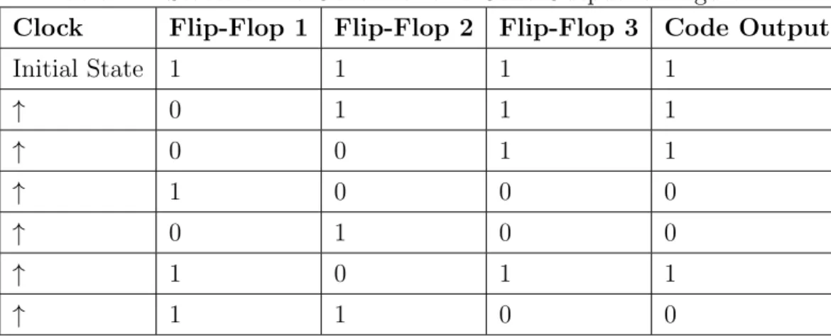
Figure 2.12: Three Stage Maximal Length Sequence Generator (n=3)
In Figure 2.12, there is a 3-stage m-sequence generator which is driven by a clock signal and producing code sequence of length N = 7 chips. By letting the initial state of the flip-flops be (1, 1, 1) among a total of seven possibilities, Table 2.1 demonstrates the resultant code output and all the states of the flip-flops at each rising edge of the clock.
Table 2.1: States of the Generator and Code Output for Figure 2.12 Clock Flip-Flop 1 Flip-Flop 2 Flip-Flop 3 Code Output
Initial State 1 1 1 1 ↑ 0 1 1 1 ↑ 0 0 1 1 ↑ 1 0 0 0 ↑ 0 1 0 0 ↑ 1 0 1 1 ↑ 1 1 0 0
As Table 2.1 illustrates, code sequence becomes (1 1 1 0 0 1 0) and it repeats itself with a period of N = 7. It is observed that the number of 1s is one more than the number of 0s in the sequence. In fact, this case is not special for a 3-stage m-sequence; instead, it is valid for all possible m-sequences and named as
zeros in an n-stage m-sequence [12]. Another property which must be satisfied by every m-sequence is the run property. It tells that every m-sequence contains one run of length n for ones, one run of length n − 1 for zeros and 2n−(p+2) runs
of length p for both ones and zeros, where p = 1, 2, ..., n − 2 [8].
An important result of these properties of m-sequence is its autocorrelation function. Autocorrelation function R(k) of any m-sequence of length N can be expressed by [12]. R(k) = 1, for k = 0 −1 N, for 1 ≤| k |≤ N − 1 (2.12)
It can be stated that when N goes to infinity, the autocorrelation function R(k) of any m-sequence becomes similar to the autocorrelation function of a WGN, hence the sequence has a noise like behavior.
The qi terms in (2.10) which are +1 or -1 where i = 0, 1, 2, ..., N − 1 are
the analog domain representations of the digital code sequence which is the m-sequence here. According to this mapping, 0 in the m-m-sequence is mapped to -1, and 1 in the m-sequence is mapped to +1. By using rectangular chip waveform φ(t) with 20 µs duration and m-sequence given in Table 2.1, chip sequence pulse waveform q(t) can be formed as in Figure 2.13.
Figure 2.13: 7 Chip Maximal Sequence Pulse, Tc = 20 µs
Before the carrier modulation, bandwidth of any m-sequence pulse q(t) can be approximated by
βω ∼=
1 Tc
(2.13)
and one bit information bandwidth can be written as
βinf o∼=
1 Tb
(2.14)
where Tb is the bit duration. By using (2.13) and (2.14), process gain in (2.7)
can be rewritten as
Gp ∼=
Tb
Tc
by using (2.13) and (2.15)
SN ROU T = SN RIN×
2 Tc
× Tb = SN RIN× 2 × Gp (2.16)
The autocorrelation function Rq(α) of a maximal length chip sequence pulse
waveform can be given by [7]
Rq(α) = 1 −
N + 1 N Tc
| a |, for | a |≤ T c (2.17)
where α is the delay parameter. The function in (2.17) is illustrated in Figure 2.14.
Figure 2.14: Autocorrelation of Maximal Length Chip Sequence Pulse
After examining (2.17) and Figure 2.14, it could be stated that autocorrelation function of maximal length chip sequence pulse becomes similar to the one which belongs to WGN while Tc is getting smaller and N is getting large. Hence, with
In Figure 2.15, an example of carrier and information modulated direct se-quence spread spectrum transmitted pulse could be seen. It uses 7 chip three stage m-sequence in Table 2.1, a rectangular chip waveform with Tc = 20 µs, a
100 kHz carrier and one bit information which has the bit duration Tb = 7Tc= 140
µs.
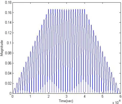
Figure 2.15: 7 Chip DSSS Transmitted Pulse
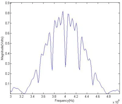
As it is observed from Figure 2.15, there are 180◦ phase shifts at times 60 µs,100 µs and 120 µs due to the transitions of the m-sequence pulse.
One sided frequency spectrum of the pulse in Figure 2.15 is illustrated in Figure 2.16. This figure shows that, one bit information, which has duration of Tb = 140 µs and null-to-null bandwidth of 2βinf o ∼= T2b = 14.29 kHz, is spread
Figure 2.16: Frequency Spectrum of of 7 Chip DSSS Transmitted Pulse
2.5
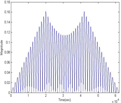
Range Resolution of DSSS Pulse
Assuming that an echo is received 1.5 ms after the transmission, cross-correlation of transmitted and received DSSS signals becomes like in Figure 2.17 and 2.18. It is observed in Figure 2.18 that peak to null time difference equals Tc = 20
µs, therefore range resolution can be written by c × Tc
2 , where c is the signal
velocity in the medium. If Tc is fixed, then range resolution does not change for
different length (or order) DSSS transmitted code sequence pulses since null-to-null bandwidths of them are fixed to T2
Figure 2.17: Cross Correlation of Transmitted and Received DSSS Signals
Chapter 3
Range Estimation Experiments
In this study, the aim of the experiments is to show that range can be estimated by using DSSS transmitted signals without any visible loss of performance even if the received signal power in the band of transmission and reception is far below the noise power level in the same band. To fulfill this purpose, several experiments were conducted and this section was prepared to share those results. After the experimental area is briefly introduced, experimental setup and devices used in the setup will be detailed.
3.1
Measurement Environment
Range estimation experiments were conducted in Yalincak Reservoir which is in Middle East Technical University Campus, Ankara, Turkey. The lake is allocated for Aselsan Inc. for underwater acoustic research and measurements.
Figure 3.1: First Arm of the Positioning System with Transducer
As shown in the Figure 3.1, in the experimental area, there is a computer controlled positioning system which holds the transducer to position it vertically and horizontally. Transducer is tied to first arm of the positioning system looking upwards and it is immersed 4.5 m into the water.
3.2
Experimental Setup
Table 3.1: Information about the Devices Used in the Experiment
Device Name and Model
Manufacturer Device Settings in the Experiment
33522A Function/Arbitrary Waveform Generator
Agilent Technologies
Burst mode with 3 s burst period. High-Z output
Low Noise Voltage Preamplifier Model SR560
Stanford Research Systems
×20 Gain and 6 dB/oct rolloff band-pass filter with cutoffs: 10 kHz and 1 mHz
DPO 7104 Digital Phosphor Oscilloscope.
Tektronix Bandwidth: 20 mHz, Coupling: AC, Sampling
Frequency: 50 MS/sec Channel 1: Transmitted Pulse, Channel 2: Received
Echo
Transmit Receive Switch Aselsan Inc.
-In order to perform range estimations between water surface and transducer, experimental setup shown in Figure 3.2 was prepared.
The flow chart of the experiment starts with Arbitrary Waveform Generator (AWG) [13]. Transmitted pulses are generated by 33503A BenchLink Wave-form Builder Basic software [14] and loaded to the arbitrary waveWave-form generator. AWG produces loaded pulse, then excites the transducer when transmit-receive switch is in transmit mode. In addition to the loaded pulse, arbitrary wave-form generator also produces a signal which controls transmit and receive mode of operations of transmit-receive switch. After transducer transmits the pulse, transmit-receive switch passes to receive mode and transducer is switched to the Low Noise Preamplifier [15]. Filtered and amplified echo as well as transmitted pulse are both monitored and recorded with Digital Oscilloscope [16]. Then, data of transmitted pulse and received echo are imported by Matlab [17] to carry out a matched filter implementation for estimating the range. A Matlab GUI prepared for this purpose is shown in Appendix A.
3.3
Experimental Methodology
In this experiment, DSSS and narrowband tone burst pulses are transmitted by using a 400 kHz transducer, TVR (Transmitting Voltage Reponse) and admit-tance of which is given in Appendix B. It has more than 100 kHz bandwidth around 400 kHz center frequency and an average TVR of 170.5 dB re 1 µP a/V across the bandwidth. For DSSS pulses, chip length is chosen as 20 µs in order to have all the energy in the signal fit into the transducer bandwidth comfortably. Generated pulses are 400 kHz carrier modulated-maximal length chip sequence pulses with N = 7, 15, 31, 63 and 127 chips and they are formed using windowed and reduced offset Gaussian chip waveform. This waveform generated by the AWG can be approximated as in (3.1), and it is depicted in Appendix C.
φ = (1 Tc )e −(t−0,5Tc)2 (√Tc π)2 − ( 1 Tc )e0,25π for 0 ≤ t ≤ Tc where Tc= 20µs (3.1)
The reason for using Gaussian chip waveform instead of the rectangular one is to reduce the side lobe level of the transmitted pulse in the frequency domain.
By this choice, a fraction of the total power which is going into the side lobes and filtered by the transducer can be reduced. The illustration which shows the difference between Gaussian and rectangular chip waveforms can be found in Appendix D.
Initially some range estimation trials are made with 7 chip DSSS transmitted pulse to determine a low drive voltage level as a starting point which is safe enough to estimate the range. For this purpose, starting from 3 Vrms, the drive
voltage is decreased to 50 mVrmslevel where 80 % successful range estimation rate
is achieved. 50 mVrms drive voltage produces 144,5 dB re 1 µP arms @ 1 m source
level with this transducer (Appendix B). The drive level is further decreased below 50 mVrms until 50 % successful range estimations are obtained. This is
repeated as pulse length is increased to 15, 31, 63 and 127 chips.
In the experiment, five different range estimation scenarios are carried out. Each scenario can be characterized by the two parameters which are electrical transmitted voltage level and amount of chips. Electrical transmitted voltage level determines the power of the transmitted pulse and chip amount determines the process gain. In the light of this information, scenarios can be listed as (7 chip-50 mVrms), (15 chip-35 mVrms), (31 chip-25 mVrms), (63 chip-18 mVrms)
and (127 chip-13 mVrms). 13 mVrms drive voltage corresponds to 132,8 dB re 1
µP arms @ 1 m source level. There are approximately 3 dB process gain increase
and 3 dB transmitted power reduction at every step. The reduction in power is compensated by longer transmitted DSSS code sequence, keeping the energy of the transmitted signal constant. Energy is the determining parameter, since the SNR at matched filter output is directly proportional to the energy of the received signal.
For each scenario, 10 pulse transmissions and receptions are carried out with 3 seconds pulse repetition interval (PRI), and records are taken for each received signal. Hence, there are 10 different received signal data for each scenario in terms of estimating the range, calculating the success rate and making discussions. After finishing the DSSS scenarios, range estimations are also carried out for tone burst transmitted pulses in order to constitute a reference for DSSS performance.
3.4
Experimental Results
3.4.1
General Information about the Experimental
Re-sults
The frequency spectrum representation of transmitted and received signals and the matched filter output results are examined for every scenario during the experiments. 7 chip-3 Vrms case is discussed in this section, which delineates the
analysis method employed in this work.
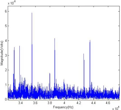
Transmitted signal is shown in Figure 3.3, where the signal is composed of 7 Gaussian chips, each of 20 µs duration. The maximal sequence used here is (1 1 1 0 0 1 0) and the carrier frequency is 400 kHz. The received electrical signal at the output of 26 dB preamplifier when this DSSS pulse is transmitted in order to estimate the range from the water surface is shown in Figure 3.4. The frequency spectrum representations of electrical transmitted and received signals are shown in Figure 3.5 and 3.6. It is possible to state that null-to-null bandwidth can be approximated to 150 kHz.
Figure 3.3: 7 Chip-3 Vrms Electrical DSSS Pulse - Transmitted Signal
Figure 3.5: 7 Chip-3 Vrms Electrical DSSS Pulse - Frequency Spectrum
Repre-sentation of Transmitted Signal
Figure 3.6: 7 Chip-3 Vrms Electrical DSSS Pulse - Frequency Spectrum
Figure 3.7: 7 Chip-3 Vrms Electrical DSSS Pulse - Matched Filter Output
The SNR improvement at the DSSS receiver can also be estimated using (2.6). In order to estimate the input signal-to-noise ratio, SN RIN, direct-path
echo power and noise power in the band of interest must be known. Noise power is estimated by measuring time domain noise data while the system is in transmit mode but not transmitting. 5 noise samples of 5 ms length are recorded with 30 s interval and appropriately filtered in order to calculate the noise power. Since separating the received signal from the noise is not always possible, to estimate direct-path echo power, following steps are performed.
• Autocorrelation of transmitted pulse is taken and its maximum point is noted as reference.
• Cross correlation of transmitted and received pulses is calculated and its maximum point is kept.
• The ratio between maximum points of autocorrelation and cross correlation results gives the attenuation amount of transmitted signal. This means that,
when the transmitted signal is divided by this ratio, received direct-path echo without noise can be extracted approximately.
For transmitted and received signals shown in Figure 3.3 and 3.4, respectively, matched filtering estimates the range as 4,58496 m assuming 1500 m/s sound velocity, and corresponding input and output SNR estimates are given in Table 3.2. SNR is improved by approximately 13.2 dB. Figure 3.7 depicts the signal at the matched filter output.
Table 3.2: 7 Chip-3 Vrms Electrical DSSS Pulse - Estimated SNRs
Estimated SNRIN for 5
Noise Data (dB)
Estimated SNROUT for
5 Noise Data (dB) Data 1 36,72 Data 1 49,95 Data 2 36,76 Data 2 49,99 Data 3 37,07 Data 3 50,29 Data 4 37,17 Data 4 50,39 Data 5 36,88 Data 5 50,10
3.4.2
Experimental Results and Discussions
Table 3.3 and Table 3.4 demonstrate the summary of the output parameters ob-tained from range estimation experiments. Table 3.3 is related to DSSS scenarios and Table 3.4 summarizes the range estimations with tone burst pulses which are used as reference. Detailed results can be examined from Table E.1 to F.5 in Appendix E and F.
Table 3.3: Summary of the Output Parameters Obtained from DSSS Range Es-timation Scenarios DSSS Scenarios Average SNRIN (dB) Average SNROUT (dB) Standard Deviation of Range Estimates (m) Mean of Range Estimates (m) 7 Chip-50 mVrms -1,43 11,80 2, 097060 × 10−3 4,5882612 15 Chip-35 mVrms -5,69 10,84 1, 458228 × 10−3 4,5873150 31 Chip-25 mVrms -7,85 11,84 10, 60744 × 10−3 4,5897916 63 Chip-18 mVrms -10,84 11,94 2, 277668 × 10−3 4,5845920 127 Chip-13 Vrms -14,75 11,06 2, 232614 × 10−3 4,5847825
Table 3.4: Summary of the Parameters Obtained from Tone Burst Pulse Range Estimations Tone Burst Pulse Scenarios Average SNRIN (dB) Average SNROUT (dB) Standard Deviation of Range Estimates (m) Mean of Range Estimates (m) 140 µs-50 mVrms 8,71 11,72 26, 21234 × 10−3 4,5666000 300 µs-35mVrms 10,06 13,07 11, 98816 × 10−3 4,5782888 620 µs-25 mVrms 9,78 12,79 112, 38993×10−3 4,6332511 1260 µs-18 mVrms 12,22 15,23 59, 38317 × 10−3 4,5904780 2540 µs-13 mVrms 12,21 15,22 277, 94573×10−3 4,5795310
It can be observed in Table 3.3 that average SNRs at matched filter input for all the DSSS scenarios are below the 0 dB level. That is to say, noise power turns out to be higher than direct-path echo power for all cases. Although the average SNR at matched filter input reduces from scenario to scenario, average SNRs at matched filter output for all scenarios are very close to each other. This is because of the process gain concept which arises due to the coded nature of the DSSS pulses as illustrated in (2.16). This result is important because it shows that even if the direct-path echo power is far below the noise power level, range estimations can still be made with very small standard deviations as shown. It can be deduced that DSSS range estimation technique can be used in an echo sounder system if LPD and accurate estimations are desired simultaneously. A system which uses low power DSSS pulses to estimate the range may not be detected by an eavesdropper system which listens the environment and monitors the frequency spectrum.
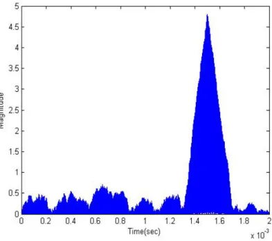
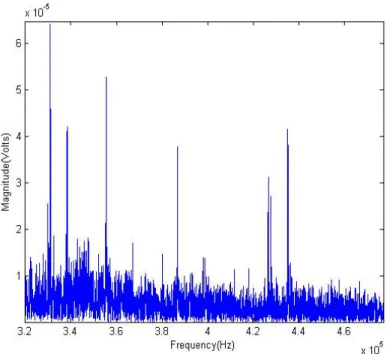
Figure 3.8, 3.9 and 3.10 demonstrate some examples of matched filter outputs from 7 Chip-50 mVrms and 127 Chip-13 mVrms DSSS scenarios. A summary for
related range estimations can be seen in Table 3.5 and detailed information about them can be found in Appendix E by tracking the left most successful estimation parameter. All of them peak at almost 6,11 ms, hence estimate almost the same range. Furthermore, the related estimations have similarities in terms of received signal and received signal frequency spectrum. From Figure 3.11 to 3.16, it can be observed that resultant direct-path echo signals are not distinguishable from the noise providing LPD. As it is previously stated this occurs due to the coded low power transmission.
Figure 3.8: Matched Filter Output for 2nd Successful Estimation of 7 Chip-50
mVrms DSSS Scenario
Figure 3.10: Matched Filter Output for 6th Successful Estimation of 127 Chip-13
mVrms DSSS Scenario
Table 3.5: Summary for Figure 3.8, 3.9 and 3.10 Related Range Estimations
DSSS Scenarios Average SNRIN (dB) Average SNROUT (dB) Mean of Range Estimates (m) 7 Chip-50 mVrms : 2nd Successful Estimation -3,18 10,04 4,58781 7 Chip-50 mVrms : 7th Successful Estimation 0,55 13,77 4,58836 7 Chip-50 mVrms : 6th Successful Estimation -13,80 12,01 4,58517
Figure 3.11: Frequency Spectrum of the Received Signal from 2nd Successful
Estimation of 7 Chip-50 mVrms DSSS Scenario
Figure 3.13: Frequency Spectrum of the Received Signal from 6th Successful
Estimation of 127 Chip-13 mVrms DSSS Scenario
Figure 3.14: Bandpass Filtered Received Signal with Passband between 325 kHz and 475 kHz from 2nd Successful Estimation of 7 Chip-50 mV
Figure 3.15: Bandpass Filtered Received Signal with Passband between 325 kHz and 475 kHz from 7th Successful Estimation of 7 Chip-50 mV
rms DSSS Scenario
Being only coded or being only low power may not be enough for LPD; a transmission scheme should bear both. For instance, in 7 Chip-3 mVrms range
estimation case mentioned in previous part, direct-path echo and its frequency spectrum can be recognized easily as shown in Figure 3.3 and 3.5. This is be-cause of the high power transmission resulting in high SNRs as demonstrated in Table 3.2. On the other hand, when low power tone bursts are utilized for range estimation, due to the low power narrowband noise in the band, LPD may not be satisfied. This situation can be illustrated by using the results of fifth successful range estimation of 2,54 ms-13 mVrms tone burst pulse shown in Figure 3.17 and
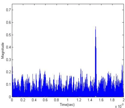
3.18. It can be observed from this figures that direct-path echo signal and its frequency content are recognizable. Furthermore, matched filter output of this example is given in Figure 3.19, and range estimation result is summarized in Table 3.6.
Figure 3.17: Frequency Spectrum of the Received Signal from 5th Successful
Figure 3.18: Bandpass Filtered Received Signal with Passband between 399,6 and 400,4 kHz from 5th Successful Estimation of 2,54 ms-13 mV
rms Tone Burst
Table 3.6: Summary for Figure 3.19 Related Range Estimations DSSS Scenarios Average SNRIN (dB) Average SNROUT (dB) Mean of Range Estimates (m) 2,54 ms-13 mVrms : 5th Successful Estimation 16,70 19,71 4,66941
As it is previously stated that DSSS transmission scheme also provides accu-rate range estimations since it uses wide bandwidth, preferably entire bandwidth of the transducer. Accuracy is related to the interference of the multipath echo signals to the direct-path echo because the time when the maximum value of matched filter output occurs can change with the interference. In order to mini-mize the amount of multipath echo signals which interfere with direct-path echo, in other words, to minimize the effects of multipath interference on the accuracy, range resolution should be kept as small as possible. When the entire bandwidth of the transducer is used in the available system configuration, range resolution becomes the smallest possible. Smallest possible range resolution means the best possible separation of multipath interference from the direct-path echo. Since the range resolution is directly proportional to the chip duration in the DSSS scheme, no matter the total pulse duration, the echo signals which are coming at least one chip duration apart from the direct-path echo can be separated from it. On the other hand, for the widely used tone burst pulse case, range resolu-tion becomes directly proporresolu-tional to the total pulse duraresolu-tion since bandwidth utilization changes with the total pulse duration. This situation is disadvanta-geous in terms of estimation accuracy when the longer pulses are used, because range resolution becomes wider. That is to say, amount of multipath echo sig-nals which interfere with direct-path echo increases and that can change the time when the matched filter output peaks. The related arguments can be observed in the following figures.
From Figure 3.20 to 3.25, it can be observed that range resolution does not change when the transmitted number of chips increases. This means that, by only adjusting the chip duration to cover the entire bandwidth of the transducer, smallest possible range resolution can be obtained providing highest possible mul-tipath resistance. As a result, it can be deduced that low power long distance ranging can be made by increasing the process gain without sacrificing the range resolution. Increasing the process gain of the low power transmitted DSSS pulse provides the necessary received signal energy for the range estimation. Theoreti-cally, as [4] states, it seems that there is no restriction on the process gain increase; however, in a real echo sounder system, processor speed and available memory for matched filtering may put a limit for maximum process gain. The other limi-tation on the maximum process gain can be underwater acoustic channel related. It is claimed in [3] and [18] that time varying nature of the underwater acoustic channel constitutes an upper limit for the process gain.
Figure 3.21: Autocorrelation of 7 Chip-3 Vrms DSSS Transmitted Pulse (Zoomed)
Figure 3.23: Autocorrelation of 127 Chip-3 Vrms DSSS Transmitted Pulse
(Zoomed)
Figure 3.25: Matched Filter Output for 1st Successful Estimation of 127 Chip-13
mVrms DSSS Scenario (Zoomed)
On the other hand, it can be deduced from Figure 3.26 to 3.27 that range resolution becomes directly proportional to the pulse duration when the widely known tone burst pulse method is used, that is to say, range resolution increases while the pulse duration increases. Therefore, optimum pulse duration should be as short as the bandwidth of the transducer permits. When the range resolution is minimized, power of the transmitted pulse must be increased in order to make long distance estimations because SNR at the matched filter output depends on the received signal energy. However, necessary transmitted pulse power may be unobtainable since the system and transducer both have a limiting peak power handling capability. Under those conditions, a compromise can be made between transmitted pulse duration and pulse power to obtain the required received signal energy for long range estimations. The disadvantage about this compromise is the increase in both range resolution and probability of detection by an eavesdropper.
Figure 3.26: Matched Filter Output for 2nd Successful Estimation of 140 µs-50
mVrms Tone Burst Pulse
Figure 3.28: Matched Filter Output for 8th Successful Estimation of 2,54 ms-13
mVrms Tone Burst Pulse
In order to have further understanding about the multipath resistance of DSSS range estimation scheme, following outputs of an assistant experiment can be examined. In the assistant experiment, the range between water surface and lake bottom was estimated. Previously, it is known that bottom of the lake bears many closely spaced scattering objects. The transmitted pulse configurations are 127 chip-3 Vrms for DSSS signaling technique and 2,54 ms-3 Vrms for tone
burst signaling technique. In Figure 3.29 and 3.30, multipath signals due to the scattering objects can be distinguished because of the small range resolution of DSSS pulse. However, for the tone burst pulse case in Figure 3.31, they are not distinguished because of the wide range resolution, hence they interfere with the direct-path echo totally behaving as if there is only one received echo signal. For the DSSS scheme, the echo which maximizes matched filter output magnitude can be taken as the direct-path echo and range can be estimated according to the time when the peak occurs. On the other hand, for the tone burst pulse in this case, exact location of the matched filter peak of direct-path echo signal cannot be determined, it may fall everywhere on the range resolution time slot.
Figure 3.29: Matched Filter Output for 127 Chip-3 Vrms DSSS Transmitted Pulse
Figure 3.30: Matched Filter Output for 127 Chip-3 Vrms DSSS Transmitted Pulse
Figure 3.31: Matched Filter Output for 2,54 ms-3 Vrms Tone Burst Transmitted
Chapter 4
Conclusion
The performance of DSSS technique in underwater acoustic ranging is studied in this work. Main motivation of this study is to make accurate range estimations with DSSS technique employing low transmitted power such that operation is both LPD and environment friendly. Two set of range estimation experiments were conducted. First experiment is the principal one, and second experiment can be named as the auxiliary experiment, supporting the first one. In the first set of experiments, transducer was immersed to approximately 4,5 m depth and positioned looking upwards (to the surface of the water). The range from the water surface is estimated. The pressure reflection coefficient is approximately -1 at water/air interface and hence this set of experiment provides performance measures when there is no loss due to bottom reflection coefficient. In the second set, the transducer was located 15 cm below the water surface looking downwards to the bottom of the lake and range from the bottom was estimated. Within the context of the first experiment, process gain was succesively increased while the transmitted power was decreased, keeping the transmitted energy almost at a constant level. The aim is to make highly accurate range estimations even if the input SNR is significantly less than zero dB. When Table Table 3.3 is considered, it can be stated that the aim was achieved since an average of approximately -14,8 dB input SNR was obtained for 127 chip-13 mVrms scenario with very accurate
eavesdropper which is very close to the transducer (the range where input SNR is 0 dB, which is less than 9,16 m) would not detect the existence of a transmitted signal for all scenarios.
When the entire bandwidth of the transducer is used, best range resolution can be obtained. In the experiments, short Gaussian chips of 20 µs duration were used, which were well within the transducer bandwidth. Therefore, multipath echo signals were easily differentiated at matched filter output as shown in Figure 3.30 which allows choosing the direct-path echo signal. Direct-path echo can either be chosen as the first distinctive echo or the echo which has the maximum magnitude. Furthermore, the capability of observing the distinctive close by echo signals at the matched filter output provides information on the insonified bottom surface. For example, it is deduced from the dispersion of echoes in the experimental results that lake surface seems flat and lake bottom contains minor corrugations.
Alternatively, these echoes, dispersed in time, can be combined either by a rake receiver as in 3G mobile communication systems or by simply increasing the chip duration slightly. The latter method is simpler to implement but yields lower range resolution.
Possible performance of DSSS echo sounding at 100 m range in sea can be estimated from experimental results. For example, if a chip sequence length of 4095 is assumed, an echo sounder system which is placed approximately 100 m below the sea surface should estimate the distance from the water surface by using 514 mVrms DSSS pulse drive voltage, when all possible loss mechanisms in
the medium are considered. First one is the absorption loss which is calculated as 105,6 dB/km around 400 kHz for sea water by using the model given in [19]. The seawater is assumed at 15◦C temperature, 8,3 pH and 35 ppt salinity in this model. The absorption loss due to 200 m two-way propagation is,
Lossabs = 105, 6 dB ×
200 m − 9, 16 m 1000 m
∼
= 20, 16 dB (4.1)
Lossspr = 20 log10
200 m 9, 16 m
∼= 26, 78 dB (4.2)
For 20 µs chip duration and 100 m range, a safe maximum for transmitted DSSS pulse length can be N = 212− 1 = 4095 chip long which corresponds to an additional 15 dB spreading gain on the contribution of 127 chip transmitted pulse. Therefore, transmitted pulse power should be increased by 31,94 dB in order to compensate the remaining loss. 31,94 dB increase from 13 mVrms corresponds to approximately 514 mVrms drive voltage for the transmitted pulse.
The frequency dependent nature of absorption in sea water can modify the chip pulse shape of wideband pulses at long ranges. In order to maintain a high correlation coefficient between the received pulse and reference pulse, it is necessary to modify the reference pulses appropriately according to the range. For the future work, this issue must be studied and resolved.
Bibliography
[1] R. P. Hodges, Underwater Acoustics: Analysis, Design and Performance of Sonar. Wiley, 2010.
[2] W. S. Burdic, Underwater Acoustic System Analysis. Prentice-Hall, 1984. [3] B. Bingham, B. Blair and D. Mindell, “On the design of direct sequence
spread-spectrum signaling for range estimation,” MTS/IEEE Oceans 2007 Conf. Proc., 2007, pp. 1-7.
[4] T. C. Austin, “The application of spread spectrum signalling techniques to underwater acoustic navigation,” IEEE Autonomous Underwater Vehicles Conf. Proc., 1994, pp. 443-449.
[5] U. Madhow, Fundamentals of Digital Communication. Cambridge, 2008. [6] M. A. Richards, Fundamentals of Radar Signal Processing. McGraw-Hill,
2005.
[7] S. Haykin, Communication Systems. 4th ed. Wiley, 2001.
[8] R. C. Dixon, Spread Spectrum Systems with Commercial Applications. 3rd ed. Wiley, 1994.
[9] D. Torrieri, Principles of Spread-Spectrum Communication Systems. Springer, 2005
[10] M. Stojanovic, J. G. Proakis, J. A. Rice and M. D. Green, “Spread spectrum underwater acoustic telemetry,” IEEE OCEANS98 Conf. Proc., 1998, pp. 650-654.
[11] J. Han, S. Kim, K. Kim, W. Choi, M. Kim, S. Chun and K. Son “A study on the underwater acoustic communication with direct sequence spread spec-trum,” IEEE Embedded and Ubiquitous Computing Conf. Proc. Vol. 2, 2010, pp. 337-340.
[12] A. Mitra, “On the properties of pseudo noise sequences with a simple pro-posal of randomness test,” International Journal of Electrical and Computer Engineering 3:3, 2008.
[13] Agilent Technologies, “Agilent 30 MHz Function/Arbitrary Waveform Gen-erators Data Sheet,” 2011.
[14] Agilent Technologies, “33503A BenchLink Waveform Builder Basic,” 2012. [15] “SR560 - Low-Noise Voltage Preamplifier,”
www.thinksrs.com/products/SR560.htm, Access date: 16/08/2013. [16] “DPO 7104 Digital Phosphor Oscilloscope,”
www.tek.com/oscilloscope/dpo7104 , Access date: 16/08/2013. [17] “MATLAB-The Language of Technical Computing,”
http://www.mathworks.com/products/matlab, Access date: 16/08/2013. [18] J. Ling, H. He, J. Li,a and W. Roberts “Covert underwater acoustic
com-munications,” J. Acoust. Soc. Am., Vol. 128, No. 5, 2010. [19] “Calculation of absorption of sound in sea water, ”
http://resource.npl.co.uk/acoustics/techguides/seaabsorption/ Access date: 16/08/2013.
Appendix A
Matlab Graphical User
Interface(GUI)
For this study, a Matlab GUI, given in Figure A.1, is prepared to process the transmitted and received data to estimate the range by using matched filtering. Transmitted, received and sample noise data files are imported and the results are visualized by pressing the “Estimate Range” button.
This software provides an interface so that chip amount and bandpass filter bandwidth can be changed dynamically by using “Enter BandPass Filter Band-width (kHz)” and “Enter Chip Amount” textboxes. After the files are selected, bandwidth and chip amount are entered. Then, “Estimate Range” button is pressed. Matched filter result is shown together with the input and output SNR results. The listbox also includes “Transmitted Data”, “FFT of Transmitted Data”, “Filtered Transmitted Data”, “Received Data”, “FFT of Received Data” and “Filtered Received Data” options to provide deep insight into the steps of the algorithm.
Matlab code for this GUI is given in the CD which is delivered to Y ¨OK (Y¨uksek¨o˘gretim Kurulu) together with a set of data files collected during the experiments. “.m” file, “.fig” file and data files must be located in the same directory in order to run the program by calling “DataAnalizi” command from
the command window of Matlab.
Appendix B
TVR and Admittance of 400 kHz
Transducer
TVR of the transducer, in dB re 1 µP arms/1 Vrms, used in this work is given in
the Figure B.1. The variation of TVR across the bandwidth is approximately between 168 and 173 dB.
The source level (SL) produced by any applied drive voltage (Vd) can be
estimated as
SL = T V R + 20 log(Vd/1 Vrms) dB re µP a (B.1)
For example 132.8 dB re 1 µP arms/1 Vrms SL is obtained for a drive voltage
of 13 mVrms, if TVR is taken as 170.5 dB on the average across the bandwidth.
The conductance and susceptance of the transducer are given in Figure B.2.
Appendix C
Gaussian Chip Approximation
Figure C.1 shows the windowed and reduced offset Gaussian chip waveform (Green Plot) which is employed in the experiments. Modulating the green plot in Figure C.1 by 400 kHz carrier gives the waveforms in Figure C.2. The wave-forms are one chip duration of the transmitted signal produced by AWG and theoretically formulated transmitted signal.
Figure C.2: Carrier Modulated Gaussian Chip Waveform Produced by Using (3.1) vs Produced by AWG
Appendix D
Gaussian vs Rectangular DSSS
Chips
Figure D.1 and D.2 show frequency spectrum of carrier modulated 7 Chip DSSS pulse with Gaussian and rectangular chips in (3.1) and (2.11), respectively. Fig-ure D.1 has wider bandwidth and smaller side lobes compared to FigFig-ure D.2. Transducer used in the thesis has a bandwidth more than 100 kHz, therefore, transducer bandwidth fits Figure D.1 more comfortably than Figure D.2.
Figure D.1: Frequency Spectrum of Carrier Modulated 7 Chip DSSS Pulse -Gaussian Chip
-Appendix E
Results of DSSS Scenarios
The results of DSSS scenarios conducted for this study are given from Table E.1 to E.5. Estimated SNRs at matched filter input and output for 5 noise data are shared together with the maximum value of matched filter output and estimated range.
Table E.1: Results for 7 Chip-50 mVrms DSSS Transmitted Pulse Successful Estimations out of 10 Estimated SNRINfor 5 Noise Data (dB) Estimated SNROUT
for 5 Noise Data (dB)
Maximum Value of Matched Filter Output(V) Estimated Range (m) 1 Data 1 -2,70 Data 1 10,52 1, 511 × 10−7 4,58803 Data 2 -2,66 Data 2 10,56 Data 3 -2,36 Data 3 10,86 Data 4 -2,26 Data 4 10,96 Data 5 -2,55 Data 5 10,67 2 Data 1 -3,38 Data 1 9,84 1, 398 × 10−7 4,58781 Data 2 -3,34 Data 2 9,88 Data 3 -3,04 Data 3 10,18 Data 4 -2,94 Data 4 10,29 Data 5 -3,23 Data 5 9,99 3 Data 1 -1,22 Data 1 12,00 1, 793 × 10−7 4,58832 Data 2 -1,18 Data 2 12,04 Data 3 -0,88 Data 3 12,34 Data 4 -0,78 Data 4 12,44 Data 5 -1,07 Data 5 12,16 4 Data 1 -0,92 Data 1 12,30 1, 856 × 10−7 4,58779 Data 2 -0,88 Data 2 12,34 Data 3 -0,58 Data 3 12,65 Data 4 -0,47 Data 4 12,75 Data 5 -0,76 Data 5 12,46 5 Data 1 -3,25 Data 1 9,97 1, 419 × 10−7 4,58623 Data 2 -3,21 Data 2 10,01 Data 3 -2,91 Data 3 10,32 Data 4 -2,80 Data 4 10,42 Data 5 -3,09 Data 5 10,13 6 Data 1 1,03 Data 1 14,25 2, 323 × 10−7 4,58649 Data 2 1,07 Data 2 14,29 Data 3 1,37 Data 3 14,59 Data 4 1,47 Data 4 14,70 Data 5 1,19 Data 5 14,41 7 Data 1 0,35 Data 1 13,57 2, 148 × 10−7 4,58836 Data 2 0,39 Data 2 13,61 Data 3 0,69 Data 3 13,92 Data 4 0,80 Data 4 14,02 Data 5 0,51 Data 5 13,73 8 Data 1 -2,88 Data 1 10,34 1, 418 × 10−7 4,59306 Data 2 -2,84 Data 2 10,38 Data 3 -2,54 Data 3 10,68 Data 4 -2,44 Data 4 10,78 Data 5 -2,73 Data 5 10,50
Table E.2: Results for 15 Chip-35 mVrms DSSS Transmitted Pulse Successful Estimations out of 10 Estimated SNRINfor 5 Noise Data (dB) Estimated SNROUT
for 5 Noise Data (dB)
Maximum Value of Matched Filter Output(V) Estimated Range (m) 1 Data 1 -5,75 Data 1 10,75 1, 592 × 10−7 4,58739 Data 2 -5,75 Data 2 10,79 Data 3 -5,44 Data 3 11,09 Data 4 -5,34 Data 4 11,19 Data 5 -5,63 Data 5 10,90 2 Data 1 -3,92 Data 1 12,61 1, 973 × 10−7 4,58649 Data 2 -3,88 Data 2 12,65 Data 3 -3,58 Data 3 12,95 Data 4 -3,48 Data 4 13,05 Data 5 -3,77 Data 5 12,77 3 Data 1 -6,49 Data 1 10,04 1, 468 × 10−7 4,59012 Data 2 -6,45 Data 2 10,08 Data 3 -6,15 Data 3 10,38 Data 4 -6,05 Data 4 10,48 Data 5 -6,34 Data 5 10,20 4 Data 1 -8,51 Data 1 8,02 1, 163 × 10−7 4,58670 Data 2 -8,47 Data 2 8,06 Data 3 -8,17 Data 3 8,36 Data 4 -8,07 Data 4 8,46 Data 5 -8,36 Data 5 8,17 5 Data 1 -4,71 Data 1 11,82 1, 802 × 10−7 4,58601 Data 2 -4,67 Data 2 11,86 Data 3 -4,37 Data 3 12,17 Data 4 -4,26 Data 4 12,27 Data 5 -4,55 Data 5 11,98 6 Data 1 -5,89 Data 1 10,64 1, 572 × 10−7 4,58727 Data 2 -5,85 Data 2 10,68 Data 3 -5,55 Data 3 10,98 Data 4 -5,45 Data 4 11,08 Data 5 -5,74 Data 5 10,79