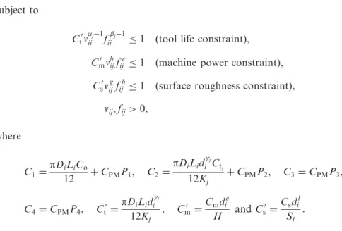
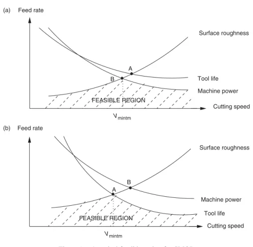
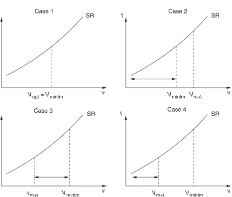
Machining conditions-based preventive maintenance

Dünyadaki uzay üsleri aras›nda en ünlü olanlar›ndan biri de Avrupa Birli¤i ülkelerinin uzay çal›flmalar›n› yürüttü¤ü Avrupa Uzay Ajans› ESA’ya ait olan Frans›z

Şair, bu kez “Ölüm ve Zaman” şiirinde Şeyh Galib’in “Ben aldım o küncü ben tükettin” dizesini, “ben aldım şiirin yılkısını/ ben ürettim...” dizelerine

kariyai Watanabe (Hymenoptera: Braconidae) – Pseudaletia separata Walker (Lepidoptera: Noctuidae) system, the protein concentration in the hemolymph of larvae injected with calyx

Minimum RPM would increase the prices of the manufacturer’s products; however, if there is sufficient inter-brand competition in the relevant market, the infra-marginal consumers

Third, the intensity and the brutality of the Armenian-Turkish nationalist confrontation in the last years of the Ottoman Empire was also due to the fact that they were the last

“the essential point is that any such group [Turkish citizens of Kurdish origin] should have the opportunity and material resource to use and sustain its natural languages

Following the analysis of the structural properties, we reveal the origin of the asymmetric distortion (Peierls instability) which transforms a metallic system into a semiconductor

The present study compared 5% topical PI with prophylactic topical antibiotics (azithromycin and moxifloxacin) in terms of effects on bacterial flora in patients