2004 International Conference on Image Processing (ICIP)
IDENTIFICATION
OF
INSECT DAMAGED WHEAT KERNELS
USING
TRANSMITTANCE
IMAGES
Zehru Catcdtepet, Enis Cetinj, E m Pearsonf
'Siemens Corp. Research Inc. 755 College
Rd
East, Princeton,
NJ 08540
tBilkent University, Dept
of
E.E. Eng., TR-06533 Bilkent, Ankara, Turkey
SUSDA, GMPRC, 15 15 College Ave. Manhattan, KS,
66502
ABSTRACT
Wc used transmitlance images and different learning algo- rithms to classify insect damaged and un-damaged wheat kemels. Using the histogram of the pixels o f the wheat im- ages as the feature, and the linear model as thc learning al- gorithm, we achieved a False Positive Rate (I-specificity) o f 0.2 at the True Positive Rate (sensitivity) o f 0.8 and an Area Under the ROC Curve (AUC) of 0.86. Combining the linear model and a Radial Basis Function Network in a committee resulted in a FP Rate of 0.1 at the TP Rate of 0.8 and an AUC o f 0.92.
1. INTRODUCTION
Infested whcat kemels cause loss of quality in the wheat products. They also cause a lot more damage if they are put into storage with other kernels. I t is important to be able to identify insect damaged kemels so proper decisions can be made about thcm.
Current methods o f insect detection such as cracking and Hotation
111,
infrared CO2 analysis [2], immunologi- cal methods [3J, NIR [4], and x-ray inspection [ 5 ] can be laborious. slow, expensive, and ineffective at distinguish- ing a sound kernel from a kernel that is internally infested. It i s possible that the use of acoustics [6] to detect insects may serve as an altemative which would allow lor recogni- tion o f kernels where the insect has already emcrged as well as those in which the insect is still living inside the kemel. In this paper wc describe a method to identify insect dam- aged kernels based on transmittance images. T h i s method i s fast and inexpensive compared with the other mcthods. Recently, reflcction images of kernels have been used for identification o f different types of grains [7].We first segmented the individual wheat kernels from the original transmittance images. Then we used the his- togram of pixel intensities from each kernel to decide if it Etnail addresses: z e h r a . cataltepe@siemens. com [email protected]".tr,[email protected]
was insect damaged or not. We used a number o f differ- ent algorithms. namely the linear model, quadratic model, k-nearrst neighbor, linear model with weight decay and Ra- dial Basis Function Network. Linear model was the best of a l l the algorithms with a False Positive Rate (I-specificity) o f 0.2 at the True Positive Rate (sensitivity) of 0.8 and an Awa Under the ROC Curve (AUC) of 0.86 0.03. A l - though the radial basis function network performed worse than the linear mode (an AUC of 0.79 0.05), a commit- tee o f a linear model and a radial basis function resulted in an improved FP Ratc o f 0.1 at the TP Rate of 0.8 and an AUC of 0.92. We also experimented with K-nearest neigh- bor model. quadratic model and linear model with weight decay (ridge regression). A l l of thcse leaming methods re- sulted in worse performance than the linear model.
2. WHEAT I M A G E S A N D FEATURES Hard red winter wheat (H2) was used to obtain the images. The insect damaged kernel images were taken from wheat infested with rice weevil and kept at ahout a moisture o f
I I%. Transmittance images were laken as 800 pixelslinch t i f images using an Epson Expression 1680 scanner. The exposure was set to 20 and gamma to 1.22.
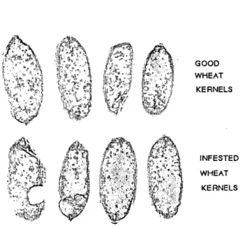
The original un-damaged and insect damaged wheat ker- nel images wcre taken all together in two different shots. First we segmented each single kernel out o f the original pictures using the blue component of the RGB. We obtained 355 good and 364 insect damaged kernels. We rotated each image so they had the maximum height and minimum width. Please see figure I for some sample images. The back- ground color was white, so we determined the borders o f each wheat image based on the background color. The re- flectance along the borders o f the image were affecting the features, so we cropped I O pixels from each pixel row on each side o f the wheat.
The histogram of red component o f the pixels colors over each wheat image was used as the input feature for the learning algorithm. The 2.56 different Red components were w t into bins as follows: If the red value was less than
GOOD WHEAT KERNELS INFESTED WHEAT KERNELS "
Fig. 1. A sample of good and insect damaged kernel pic-
tures.
or
equal to 80 the pixel wils added into bin 0. If it was larger than 250 it was added into the last bin. (Since there were almostno
pixels with Red component 80, we chose the limit 80. We merged Red value 255 into the bin that con- tained 25S25-1.) Otherwise, the pixel was added into a bin in-hetwecn, each bin being responsible for 5 different red values resulting with a total of 36 input Features. Since the bins with Red value less than 8 0 were almost always empty, we chose to put all pixels with a Red component of less than 80 into one bin. Since there would be only one Red value (255) in the last bin, we decided to add that to the bin for 250-254. Figure 2 shows the mean and standard deviation of features for all the available data. We assigned output 0 to the good kernels and I lo the insect damaged kcmels.In addition to the histogram features, we tried two other features: the minimum, m u i m u m and majority over 3x3 rectangles and the mean on the center of the wheat. We also tried using, in addition to the Red histogram, mean of Red, Green and Blue, hue, saturation, brightness and mean
x
andy of CIExy.
However, the results didn't improve,so
we don't report them hem.3.
LEARNING ALGORITHMS
We used two examplar-based algorithms: k-Nearest Neigh- bor and radial basis function (RBF) network
[XI,
as well as two model based algorithms: linear and quadratic models. In order to see if regularization would help with the linear model, we also tried weight decay. The input features for all the algorithms were ER"G
and the corresponding out- puts were y E {-1,l). The inputs were normalized to haveFig. 2. The mean and standard deviation of the input fea-
tures for good and insect damaged kernels.
sample mean 0 and standard deviation I for each input di- mension on the training set.
In order to get reliable figures on algorithm performance, we used cross validation. We randomly partitioned all the available data into a training and a test set. The training set used 9 0 6 of data from each class and the test set used the remaining IO%. We repeated the partitioning I O times.
We estimatcd the model performance using the ROC (Receiver Operating Characteristics)
[9]
and the Area Un-der thc ROC curve (AUC) [IO] o n the test set. In order to obtain different False and
True
Positive rates on the ROC curve, we varied the threshold of each learning algorithm.Linear Model: Let
A N
(38+1) contain training in-puts preceded by I and
bN
contain the outpuls yifor all the
N
training examples. The linear model is obtained by solving for w,~.,
in the equationA%
=-
b. In order to solve this equation we need to invert ATA. SinceA
was not full rank,A T A
was not in- vertible. We used singular value decomposition [ I I ]with E
=
0.001.If thc output for a test case was smaller than a cer- tain threshold we classified it as good and otherwise we classified it as insect damaged. Each threshold for the linear classifier corresponds to a p i n t on the ROC curve (i.e. a certain
FP
and T P rate).In
order to get different points on the ROC curve, we varied the threshold for the output from -2 to 2 in stepsof
0.1. For a certain threshold t and for a certain input, i f the output of the linear model was more than the threshold, the input was classified as insect damaged, otherwise it is classified a$ good. When we varied the
threshold between -2 to 2 we were able to draw the complete ROC curve, that starts at T P and FP rates of 0 and ends at TP and FP rates of I.
Radial Basis Function (RBF) Network: We used
the RBF network described in [ X I choosing the first layer weights step-wise as the training example with the worst training error. We used 20 basis units. RBF network's first layer does a non-linear transfurmation of the inputs and then the output is determined as a linear combination of the basis function outputs. We used thresholds as in the linear model to get dif- ferent ROC curve points.
Linear Model and RBF Network Committee: We
used a linear combination ofthe RBF network and the linear model outputs as the output of the committee and the same thresholds to get ROC curve points.
Quadratic Model: We used the inputs used for the
linear model and also the multiplication of each input with another input.
We used thresholds as in the linear model to get dif- ferent ROC curve points.
k Nearest Neighbor: This algorithm needs to store
all training data. In order to classify a new data point, first the K closest data points (K neighbors) in train- ing data are detcrmincd. The new data point is clas- sified as positive or negative, based on the count of positive and negative count in the K neighbors. The number K determines the smoothness of the
k
Nearest Neighbor classifier [XI. AsK
increases the classifier does a smoother interpolation. We used 5 ,IO, 15 and 20 as the values of K in our experiments.. In order to get different points in the ROC curve, we varied the threshold for the output from 0 to I . We computed the mean of the labels of the K nearest neighbors. If the mean is less than the threshold. we classified a test case as good and otherwise as insect damaged.
Linear Model with Weight Decay Weight decay, ridge
regression and shrinkage aim at reducing the weights and hence obtaining simple models that do not over- fit the training data. The weight decay solution is Bit
- =
(ATA
+
XI)-'ATy. The selection of the weight decay parameter X isvery important. If X is very small. the wcight decay doesn't change the solu- t is too large, the solution gets smaller in size at the expense of bad tit to the data.We used thresholds as in the linear model to get dif- ferent ROC curve points.
Table 1.
Lcarning Algorithms
Area Under ROC Curve (AUC) for Different
4. RESULTS
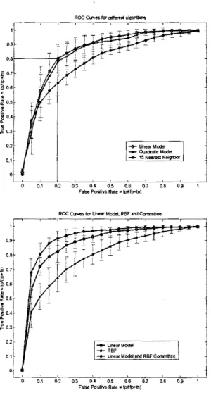
For each of the I O training-test set partitioning of the avail- able data, we used the training set to train the learning algo- rithm. We then used the test set to compute the ROC (Re- ceiver Operating Characteristics) [12, 9, 131 curve for each parti timing.
We interpolated the ROC CUNC for each partitioning
and reported the mean and standard deviation of the T N ~ Positive Rate (sensitivity) for each False Positive Rate ( I - specificity) value for each learning algorithm CY]. The mcan and the standard deviation on the ROC C U N ~ gives us a bet- ter idea on the performance of an algorithm. In order to get a reliahle mean, we discarded the ROC curve with the max- imum and minimum AUC and computed the average ROC curve using the X remaining ROC curves. Please see table 1 and figure 3.
Because of its simplicity and performance linear model seems to be the best single algorithm. The nearest neighbor was the worst algorithm, regardless of the
K
of the nearest neighbor. The KBF and linear model committee performed the best.5. DISCUSSION
We used a number of learning algorithms
to
classify good and insect damaged wheat kernels and we found out that the regularized linear model performed the best. Additional in- formation about the kernels such as reflectance images or as compression force or conductance measurements [6] could be used to improve performance of a single classifier. An- other approach is to train different classifiers with each o f these features and then combining them [ 141.,r
j4
Fig. 3. Performance of Different k a m i n g Algorithms.
6. REFERENCES
[ I ] G.E. Russell, “Evaluation of four analytical methods to detect weevils in wheat: granary weevil, sitophilus granarius in soft white wheat,” Journal
of
Food Pro- tection, vol. 5I ,
pp. 547-553, 1988.[ 2 ] W.A. Bruce, M.W. Street, R.C. Semper, and
D.
Fulk, “Detection of hidden insect infestations in wheat by infrared carbon dioxide gas analysis,’’ ARS bulletin, vol. July, AAT-S-26, 1982.[3] EA. Quinn, W. Burkholder, and G.B. Kitto, “Im- munological technique for measuring insect contam- ination of grain:’ Journal of Economic Entomology, vol. 85(4). pp. 1463-1470, 1992.
[4] F.E. Dowell, I.E. Throne, and J.E. Raker, “Automated
nondestructivc detection of internal insect infestation of wheat kernels by using near-infrared spectroscopy,” Jourriol of Economic Entomolugy, vol. 9 I (4), pp. 899- 904, 1998.
[SI R.A. Stermrr, “Automated x-ray inspection of grain for insect infestation:’ Trunsactions ofthe ASAE., vol. 15, pp. 1081-1085. 1972.
[6] T. Pearson, D.L. Rrabec, and C.R. Schwartz, “Auto- mated detection of internal insect infcstations in whole wheal kemels usign a perten skcs 4100,’’ Applied Engineering in Agricultirre, vol. 19(6), pp. 727-733, 2003.
[71 N.S. Visen,
D.S.
Jayas. J. Paliwal, and N.D.G. White, “Comparison of two neural network architectures for classification of singulated cereal grains;’ Canadian BioSystenis Engineering, vol. 46, pp. 3.7-3.13,2004. [81 C. M. Bishop, Neural Networksfor Partern Recogni-tion, Clarendon Press, Oxford, 1995.
[ Y l E Provost, T. Fawcett, and R. Knhavi. “The case against accuracy estimation for comparing induction algorithms,” in P m c . 15th International C o i f on Mrr-
chine Learning. 1998, pp. 445453, Morgan Kauf- mann.
[IO] A. P. Bradley. ‘The use of the area under the roc curve in thc evaluation of machine learning algorithms,” Pat- tern Recognition, vol. 30, No. 7, pp. 1145-1 159, 1997. [I I ] W. H. Press, W. T. Vettcrling, B. P. Flannery, and S. A.
Teukolsky, Numericol Recipes in C: The Ar? of Scien-
tific Computing, Cambridge University Press, 1992.
[ 121 C. E. Metz, “Basic principles of roc analysis:’ Semi- nars in Nuclear Medicine, vol. 8, pp. 283-298. 1978. [ 131 M. H. Zweig and G. Campbell, “Receiver-oprating characteristic (roc) plots: a limdamental evaluation tool in clinical medicine,” Clinical Chemistry. vol. 19, pp. 561-567, 1993.
[ 141 J. Kittler M.