c52S:!lUÄ!. :Saia;aF SüüSRSS
:
■
СОйШ®
Ш!·
J
ШВ JÄ- ί
Й ô Û i ï M Ê S i S D Й Ѵ р { | ѵ и £ щ , т с д ] ь л 2Â.îHESİS РНЕЕЕВД В?
4, i, ''--^ - г ¿ Ь» ‘1
П' І-Г- ■ ѴгѴ'і d ^ îir Æі i ^ j е € п D F а ш с ш с в *ѴГ>'S3CÄ SCiBïCES
а ш
т
ршлшіш
of
e s
йШшетЕШ
гОйШВЕВЩОг
е т ш ÖF Ееоюшсо
ив
'8οι
á l f ' г Và ѵЭііилЬкО ,U ‘- m m m ^ á v ш т i L· U^^rSá i( I Ό o Ij/PREDICTIVE RESIDUAL SUM OF SQUARES COMPARED WITH J AND JA
IN NONNESTED HYPOTHESIS TESTING
A THESIS PRESENTED BY YENER KANDOGAN TO
THE INSTITUTE OF ECONOMICS AND
SOCIAL SCIENCES
IN PARTIAL FULFILLMENT OF THE
REQUIREMENTS FOR THE DEGREE OF MASTER OF ECONOMICS
BILKENT UNIVERSITY MAY 1996
I certify that I have read this thesis and in my opinion it is fully adequate in scope and in quality, as a thesis for the degree o f Master o f Economics.
I certify that I have read this thesis and in my opinion it is fully adequate in scope and in quality, as a thesis for the degree o f Master o f Economics.
Akoc. P ro f Osi an Zaim
I certify that I have read this thesis and in my opinion it is fully adequate in scope and in quality, as a thesis for the degree o f Master o f Economics.
Assist. Prof. Erdem Başçı
ABSTRACT
PREDICTIVE RESIDUAL SUM OF SQUARES COMPARED WITH J AND JA
IN NONNESTED HYPOTHESIS TESTING
YENER KANDOGAN MASTER OF ECONOMICS Supervisor: Prof. Dr. Asad Zaman
May 1996
In nonnested hypothesis testing, J test suggested by Davidson and MacKinnon (1981) and JA test suggested by Fisher and McAleer (1981) are two common tests used to evaluate hypotheses. In this thesis, we first give the necessary background for J and JA tests in nonnested hypothesis testing and the literature survey on these issues. We then compare the performances of J and JA tests with Predictive Residual Sum of Squares method. Monte Carlo experiments are carried out to compare these tests in testing Quadratic versus Leontieff models and also Linear versus Log-Linear models, where we find that Predictive Residual Sum of Squares method has superiority over the other tests mentioned in terms of power. In the end, a real case study testing different consumption function theories for 1987-1995 period in Turkey is presented.
Key Words; Predictive Residual Sum o f Squares, J test, JA test, nonnested hypothesis testing
ÖZET
İÇİÇE GEÇMEMİŞ HİPOTEZ TESTİNDE TAHMİNİ HATA KARELERİNİN TOPLAMI
METODUNUN J VE JA TESTLERİ İLE KARŞILAŞTIRILMASI
YENER KANDOĞAN
Yüksek Lisans Tezi, İktisat Bölümü Tez Yöneticisi: Prof. Dr. Asad Zaman
Mayıs 1996
İçiçe geçmemiş hipotez testinde Davidson ve MacKinnon (1981) tarafından önerilen J testi ve Fisher ve McAleer (1981) tarafından önerilen JA testi sık kullanılan iki testtir. Bu tezde ilk önce içiçe geçmemiş hipotez testinde kullanılan J ve JA testi için genel bilgi ve bu konularda yapmış olduğumuz yayın araştırması veriliyor. Sonra J ve JA testlerinin performansını tahmini hata karelerinin toplamı metodunkiyle karşılaştırılıyor. İkinci dereceden modellerin Leontieff modeliyle, Logaritmik modellerin Lineer modellerle test edilmesinde Monte Carlo deneylerini kullanarak bu test teknikleri karşılaştırıldı. Bu deneyler sonucunda tahmini hata karelerinin toplamı metodunun diğer testler karşısında güç bakımından üstün olduğu bulundu. Son olarak gerçek verileri
♦
kullanarak 1987-1995 dönemi Türkiyesi için değişik tüketim fonksiyonları teorileri test edildi.
Anahtar Sözcükler: Tahmini Hata Karelerinin Toplamı, J testi, JA testi, İçiçe Geçmemiş Hipotez Testi
ACKNOWLEDGMENT
I would like to express my gratitude to Prof. Dr. Asad Zaman for his valuable for their patience and for their support in harsupervision and for providing me useful comments. Special thanks to all my iiiends d times.
CONTENTS Abstract
Özet
Acknowledgments Contents
1. Why Comparing Models ? 7
2. Comparing Nonnested Statistical Models 10
3. Preliminaries for J and JA test 13
4. J and JA test 16
5. Predictive Residual Sum o f Squares Method 20
6
. Previous Researches on Power Comparison o f Nonnested Models 227. Data Set 26
8
. Power Comparisons 269. The Results 28
10. Nonnested Tests in Empirical Works 30
11. Empirical Work; Turkish Consumption Function 32
A. Abstract 32
B. Theoretical Work 33
C. Empirical Estimation 36
D. Conclusion and Results 39
12. Appendices 42
1. W hy C om paring Models ?
Econometricians build models for two main purposes: estimation and inference. In such practices, a linear statistical model with parameters is generally assumed. This approach is consistent with the sampling process, by which the observations are drawn. Every applied econometrician has had the experience o f estimating a regression model which at first glance, seemed to be satisfactory, but later turned out to be invalid. In practice, true statistical models are very rare. The nature o f economic data makes this situation inevitable. The right-hand side variables, that is, the explanatory variables are usually collinear. This is because of time-series data exhibiting the same trends, the same business cycles.
Then, a reasonable judgment is that most o f the statistical models used by economists so far are invalid. This fact casts doubt upon the estimations and inferences that are being built on them. But, first the roots of the problem must be identified. What are the sources o f misspecification yielding such judgment? How can they be detected? What are the ways of avoiding them? Actually, there are many reasons causing model misspecification. Omission o f a relevant explanatory variable or misinclusion o f some explanatory variables are two most likely reasons for model misspecification. To detect and avoid such defects, some variable selection procedures that includes both discrimination among nested alternative models and testing of separate (nonnested) models are developed to solve model misspecification problems.
At this point, a differentiation between nested and nonnested models needs to be done. Two statistical models are nested when one o f them is a special case o f the other, with some parameter restrictions. For example, Cobb-Douglas production function is nested within Constant Elasticity o f Substitution (C.E.S.) production function. Cobb-Douglas production function is a special case of Constant Elasticity o f Substitution production function, obtained with some parameter restrictions. C.E.S. production function with unity elasticity of substitution reduces to a Cobb-Douglas production function. Two models are said to be nonnested when one o f them can not
constitutes an example of two nonnested models. Here, log-linear statistical models are actually multiplicative models or exponential models, linearized by taking logarithm o f both sides. Clearly, linear models can not be obtained from log-linear models merely by some parameter restrictions.
Model misspecification, or rather, selection o f a statistical model and nonexperimental model building are very old problems in econometrics. Many research efforts have been devoted in this area. As a result o f these researches many criteria, testing mechanisms, search processes and empirical rules came out to help the economists in selecting appropriate statistical models. These procedures and rules are discussed in recent articles or books o f Gaver and Geisel (1974), Hocking (1976), Thompson (1978), Learner (1978), Amemiya (1980), Maddala (1981), White (1982,1983), MacKinnon (1983), Sawyer (1980), McAleer (1984) and Doran (1993) among others.
In this literature, some criteria and rules are suggested in adjusting a design matrix, more explicitly, in deleting or adding explanatory variables. In this framework, it is usual to appeal to economic theory for guidance in specifying econometric models. So, in all of these studies main emphasis is made on the importance o f economic theory in forming explanatory variables matrix.
Economic theory helps a lot in narrowing the range o f explanatory variables as well as in determining possible functional forms. It has much to offer the researcher in describing which economic variables should be considered and the direction o f possible relationships between the variables. But theory rarely suggests one model to explain a particular phenomenon. Often there are rival theories, and even when there are not, a single theory may be compatible with several functional forms, or some handful o f stochastic specifications. Besides, unfortunately, economic theory, treating most variables symmetrically, is of little help when the researcher is at the stage o f quantitative analysis, where the appropriate functional form should be specified. When faced with several competing regression models, it is simply necessary to choose the model which is best. In order to do this an applied econometrician would
use a model selection criterion. O f course, the econometrician usually does not know whether any o f the competing models could conceivably be true. So, specification o f each o f the available models should be tested. Tests for heteroskedasticity, serial correlation, parameter stability and other criteria play important roles in this context. But, it should be noted that the tests mentioned above do not make use o f the information that the model tested is only one of the several models to explain a certain phenomenon. Some of the rules or criteria in selecting between nested statistical models are:
-Orthodox (Classical) Hypothesis Testing Framework: F test. Mean Square Error Norm test,
-Residual Sum of Squares Rules: Coefficient o f Determination: r2. Adjusted Coefficient o f Determination: R ^ , Amemiya’s Unconditional Mean Square Error Criterion: PC, Mallows Conditional Mean Square Error Prediction Criterion Cp,
-Information Criteria: Akaike Information Criterion AIC, Sawa’s Criterion BIC, Schwarz Criterion SC, Chow Criterion are some examples. The fundamental notion in this approach is the following. The information criterion seeks to incorporate in model selection the divergent considerations of accuracy o f estimation and the best approximation to reality. Thus, use of this criterion involves a statistic that incorporates a measure o f the precision o f the estimated a measure o f the rule o f parsimony in the parametrization of an econometric model. In this context, the adequacy o f an approximation to the true distribution o f a random variable is measured by the distance between model of reality and the true distribution.
-Bayes Criteria: Jeffreys-Bayes Posterior Odds Ratio is an example for this approach. Gaver and Geisel (1974) developed a framework for using the posterior odds ratio and a basis for discriminating among models. Fundamentally, the posterior odds ratio depends on the prior odds ratio, the compatibility o f the prior distributions and the maximum likelihood estimates. This criterion makes use o f a ratio o f the determinants of the two design matrices and a ratio o f likelihoods. Consequently, a
-Stein Rules: Basically, including some extraneous variables in the design matrix or excluding any of the important explanatory variables from the design matrix conditions the precision and the bias, with which the coefficients o f explanatory variables are estimated. In bias-variance choice within Stein rule context, the data are used to determine the compromise between bias and variance and the appropriate dimension o f the design matrix.
2. Comparing Nonnested Statistical Models
The primary concern o f this thesis is the comparison o f nonnested models. Cox, Atkinson, Quandt, Pesaran and Deaton, Davidson and MacKinnon, Fisher and McAleer worked on this area and they developed some tests, which are variants o f likelihood ratio test. The initial work in this subject is done by Cox (1961). Then, Pesaran (1974) extended the researches by Cox to include the regression model and concentrated on the autocorrelated disturbance case. Thereafter, Pesaran with Deaton (1978) extended his early results so that there is no need for the assumption o f linearity in the models. So, testing o f competing nonlinear models can also be done. Afterwards, Atkinson (1970) suggested a procedure that combines the nonnested models into a general model, which constituted an important pace in nonnested hypothesis testing. Dastoor (1983) noted an inequality between Cox and Atkinson statistics. Fisher and McAleer (1981) modified the Cox test for linear regressions. In the mean time, Davidson and MacKinnon (1981) suggested processes for model specification testing, known as J test, which are linearized versions o f Cox test. These are closely related to the nonnested model testing o f Pesaran and Deaton (1978), named as JA test.
There are many cases in applied econometrics, where there is a need for testing nonnested hypotheses. At this point, let’s clarify a point. Since to each hypothesis, there corresponds a unique model, the terms hypothesis and model will be used synonymously. In nonnested hypothesis situations, one model can not be obtained from the other model by simply imposing some restrictions or by making some approximations. But what are the situations that nonnested hypothesis testing
will be needed? The following are some instances faced in applied econometrics, where nonnested models are appropriate:
-Functional Form Differences: In general, models with different functional forms can not be nested. Quadratic and Leontieff production functions provide an example to this case.
-Variable Definition Differences: For example, models may use different definitions for expected price or interest rate.
-Different Theories: In consumption function, models o f different theories are examples for this case. Absolute Income Hypothesis, Relative Income Hypothesis, Permanent Income Hypothesis, Life-Cycle Hypothesis can be tested using nonnested hypothesis tests.
-Linear and Log-linear Models: Testing Cobb-Douglas production functions with additive or multiplicative error terms is an example for this case.
Despite many possible situations as above. Is nonnested hypothesis testing widely used in practical applications? In agricultural economics literature, for instance there are many applications, where one should include nonnested hypothesis testing as part o f the general specification testing program, but it is not usually considered. American Journal o f Agricultural Economics (1990-1991 issues) state out some important observations from applied research:
-Without any theoretical justification models are usually used in log-linear form,
-A comparison between models with same dependent variables and different explanatory variables is usually made,
-Hypotheses with different functional forms are compared in an ad-hoc way. Until recently, a misleading approach was subject to nonnested models. In this approach the primary emphasis was on discrimination rather than testing. That is a very deceptive point o f view. Basically, model selection criteria are appropriate when one wishes to choose one out o f a group o f competing models. Here, the
parametrization. Within that framework a best model was chosen depending on its performance or sample explanation. R^, R ^ and Akaike Information Criterion were mainly used for this purpose.
But, actually there are two fundamental differences between discrimination and testing. Since one best model is sought, the discrimination process will always lead to choosing a model. In testing framework, however, all o f the models can be rejected as inadequate to explain the variations in the dependent variable. Also, in testing framework probabilities are attached to the misrejection o f null hypothesis, whereas, in discrimination process, even though such probabilities exist, they are difficult to obtain.
On the other hand, nonnested hypothesis tests are tests o f model specification. The only important difference between nonnested hypothesis tests and more classical procedures is that they rely on the existence o f nonnested alternative models. Orthodox tests, in this respect ignore the availability o f a nonnested alternative hypothesis. The results o f applying such tests to two competing models may be that one model can be rejected while the other can not, but it may just, as well, be that both of the models , or neither model can be rejected. Thus testing each model against the evidence provided by the other can not allow the researcher to choose one o f the competing models. What it can do is to provide evidence that one o f the models or both o f the models are misspecified.
It must again be stressed that, nonnested model tests are specification tests. They make use o f alternative models. Using the information about the alternative, they test whether the null can correctly predict the performance o f the alternative. In nonnested hypothesis case, there is a data system and a system of alternative models. Since alternative models are nonnested, they are unranked as to generality, in contrast to nested models. Nested models can be ranked among themselves, by the number o f additional explanatory variables added to a core model. In normested case, each o f the models is considered equally likely. Separate tests of each pair of hypotheses is made. In each case, a check is made to see whether the performance o f one model is
consistent with the truth of the other model. This process is repeated for the truth o f each available model. It is clear that in comparing two nonnested models, four outcomes are possible:
-Both o f the hypotheses are rejected as inadequate,
-The first model is accepted and the second is rejected as inadequate, -The second model is accepted and the first is rejected as inadequate, -Both models are accepted.
Note that, the Discrimination Criteria should be used only with the last outcome, where both models are considered as adequate.
3. Preliminaries for J and JA tests
Suppose that we have two competing hypotheses HO and HI about a dependent variable y. Suppose further that the true data generating process o f у is also known. For clarity, lets assume data generating process to be:
Hq: y=XoBo + UQ where uo~N(0,ao^It)
Let the alternative model be o f the form: H ] : y ^ X j B i + uj where ui~ N (0 ,ai2 lt)
The parameters Bq and are known and the parameters B j and, have to be estimated. Here, the estimated, is taken as a measure o f model performance. The ability to predict model performance according to the data generating process o f the dependent variable is a major concept in normested model testing, which is first used by Cox (1961). In the test for nonnested models implemented by Cox, a variant o f Neyman-Pearson likelihood ratio test which compares the value o f this test statistic with its expected value is used. The basic idea o f this procedure is that one may test the validity o f a null hypothesis about how a data set was generated, by comparing the observed ratio o f the values of the likelihood functions for the null hypothesis and for some nonnested alternative hypothesis with an estimate o f the expected value o f this likelihood ratio if null hypothesis were true. If alternative hypothesis fits either better or worse than it should if null hypothesis were true, then null hypothesis must be
false. Сох considered the asymptotic distribution o f a function o f the generalized log likelihood ratio, in his procedure.
For the case where the data generating function o f у is not known, the method is similar, but with slight differences. In short, this procedure for this case works as follows: First one o f the models is assumed to be the data generating process and the performance o f the other model is predicted on the basis o f first model. If the actual performance o f the estimated, is close to its predicted performance, a confirmation o f the first model can be made. In contrast, if the actual performance o f the estimated, jg not close to its predicted performance, the first model will be rejected as inadequate. In determining the closeness o f estimated performance to its predicted performance, significance level method is applied. A significant value for the test statistic suggests rejecting the first model. Here, it is crucial to note that rejecting the first hypothesis has no implications whatsoever on the adequacy o f the other model.
So, in summary, two tests will be performed, where each model will have a chance o f being assumed to be the data generating process. The outcome o f these tests will determine whether the data is:
-consistent with the first model, -consistent with the second model, -consistent with neither models, -consistent with both models.
As previously noted, when two models are tested against each other, there are four (even nine) possible outcomes (nine outcomes if one distinguishes between rejection in the direction o f alternative model and rejection in the opposite direction). Therefore, interpreting the results of such a pair of tests may seem complicated. For a detailed discussion on this matter see Fisher and McAleer (1979). However, for practical purposes interpretation of results is not particularly difficult. If none o f the models is rejected, the data does not allow us to say that either is false. If one model is rejected and the other is not, then the set of models that are worth further examination
has been reduced in size. This is a quite useful outcome for practical purposes. At this point, it should be remembered that there may be many nonnested alternative models. Furthermore, if both models are rejected , then the set o f models has been reduced in size even more. Indeed, if there are no models around, the applied econometrician should presumably invent some. In this particular situation, the signs o f the test statistics may be useful. This is because, in such a case, the sign o f tests statistics will tell us whether one should look for a model that combines features o f both models rejected, or for a model that moves away from one o f the models.
Furthermore, there is also another important remark that should be made. One should note that in the case of nonnested models, there are many alternative hypotheses. Therefore, rejecting one of the models as null hypothesis does not necessarily imply that the other model is acceptable.
Now, it is time to set out an important preliminary concept in J and JA tests: A convenient way o f comparing nonnested models is to add another explanatory variable to the model being tested and examine the associated t-statistic. As noted earlier, the rejection o f the first model does not imply anything about the adequacy o f the other model, even if the added variable is derived from the other model. Then, the only implication o f this is that the augmenting variable is correlated with the variable(s), which are incorrectly omitted from the first model. In this testing procedure the model is tested against a nonnested alternative. Since each o f the models is drawn from the economic theory, there is good reason to believe that the augmenting variable is highly correlated with the incorrectly omitted variables in the first model.
4. J and JA tests
J test is a linear version of the test proposed by Cox. It has been suggested by Davidson and MacKinnon (1981). Lets assume two competing hypotheses:
Hq: y=XoBo + UQ where uo~N(0,ao^It)
Assume that Xq and X j are independent. An immediate way o f testing these models is to combine them in a composite form given as:
He: y^XoBo + X l B ] + u
Then, an F test carried out to test whether Bq=0 or Bi
=0
will imply H] or Hqrespectively. However, problems arise when power o f these test is considered: If both Xq and X j have large number o f columns, that is, both models use numerous explanatory variables, then the degrees o f freedom in the numerator o f the F-statistic will be large, consequently the power will be diminished. Furthermore, if the assumption o f linearly independent Xq and X \ is relaxed in such a way that, Xq and
X \ are highly collinear, then multicollinearity problem will arise. Then, the power o f this test will be further reduced. With such a low power this test may fail to reject none of the models even if they are both inadequate.
Davidson and MacKinnon (1981) solved these problems by considering embedding the models by a more general way: by taking the weighted average o f the models using a fixing parameter L:
y=(l-L)XoBo + LXiBi +u
Davidson and MacKinnon replaced the X i B j by its estimate y = (I-M i)y , where M i= X i(X /X i)'' X /. Therefore, the above equation can be written as:
y=(l-L)XoBo + L y + u
Since the estimate o f y is asymptotically independent o f the error term, Davidson and MacKinnon proposed to test if L equals to 0 to see if Hq is true by
using a likelihood ratio or even a conventional t test. They named this process as J test.
An exponential type and constant elasticity o f substitution type combination o f deterministic components of the regression models could also be considered. For competing linear regression models, Davidson and MacKinnon (1980) conjecture that the various combinations yield similar results, but they recommend the linear combination for its simplicity. Therefore, a choice between the numerous ways o f combination o f models is a topic for further research.
JA test suggested by Fisher and McAleer (1981) is in principle very similar to J test. Both J and JA tests use an artificial regression, which is obtained by augmenting the null hypothesis by a variable. This variable is obtained by some regressions using the alternative hypothesis as well. Since both o f the tests are one degree o f freedom tests, their power is higher than the direct composition approach considered at the beginning. Pesaran justified this case in his studies (1982).
The difference between the J test and the JA test is that the augmenting variables added to the null hypothesis are different. In J test, X i B j is replaced by (I- Mi)y. Thus, J test requires only two regressions. However, in JA test, X i B j is replaced by (I-Mi)(I-Mo)y. Therefore, three regressions must be carried out for JA test. But, the advantage of JA test is that when the models in consideration are linear and the disturbances are normal, this test is exact. Even with small samples, this test produces tests o f correct size. However, J test is not exact in this sense. With small samples, J test may reject a true model too often. In spite o f this disadvantage o f J test, Monte Carlo evidence proves that J test is a more powerful procedure compared to JA test.
Let’s at this point, state a deficiency o f using J and JA tests. O f course, a statistical outcome could be the acceptance o f the composite model. This is at the one hand and at the same time an advantage and a disadvantage o f using J and JA tests. In J and JA tests, the acceptance o f the composite model is not possible. Thus, on the one hand, using J and JA tests has an advantage in that the composite model itself may not be conceiveable, whence one is not forced by the data to accept an inconceivalbe proposition. On the other hand, it has a disadvantage in the case where the composite model may have some hidden meaning. For example Cox (1961) points out that the combined model may lead to an adequate representation o f the data when both component hypotheses are false. That is, if the artificial model is in some sense closer to reality than either o f the component models, the fact that we can not accept it is an obvious drawback o f using J and JA tests as numerical methods o f identification.
Although the exponential weighting o f likelihood functions is naturally appealing, there are certainly other methods available for nesting alternative models within a more generally framework. This raises the interesting question o f whether the concept o f nonnested hypotheses is itself more than a thoroughly practical artifact. It could be argued, for example, that the reasonable competing hypotheses are just special cases o f some more general system, special components o f which are the individual null and alternative hypotheses. Therefore, consideration o f the form o f nesting o f the competing hypotheses may then be as important as the actual testing procedures themselves.
We are now in a position to spell out the simple steps in J and JA tests in testing two competing linear models;
Model 0: y=XoBo + uq
Model 1: y =X iB i + u\
J test:
Null hypothesis is Model 0.
-Regress y on X ], and get the predictions y l ,
-Regress y on Xq and y l ,
-J-statistic is the t-value o f the coefficient o f y l .
Null hypothesis is Model 1.
-Regress y on Xq, and get the predictions y O,
-Regress y on X j and y O,
-J-statistic is the t-value o f the coefficient o f yO .
JA test:
Null hypothesis is Model 0.
-Regress y on Xq to obtain predictions yO ,
-Regress yO on X j to obtain predictions yol , -Regress y on Xq and y o l,
Null hypothesis is Model 1.
-Regress у on X j to obtain predictions y l ,
-Regress y l on Xq to obtain predictions y l
0
, -Regress у on X j and7
IO,-JA-statistic is the t-value of the coefficient o f 10.
The below are the steps that must be carried out for J and JA tests in testing competing linear versus log-linear regression models, which is suggested by Bera and McAleer;
Model 0: log y=XQB0 + uq
Model 1: y =X i B l + uj
J test:
Null hypothesis is Model 0.
-Regress у on X
2
, and get the predictions y l ,-Take the logarithm o f y l , and get log y l ,
-Regress log у on Xq and log y l ,
-J-statistic is the t-value o f the coefficient o f log y l .
Null hypothesis is Model 1.
-Regress log у on Xq, and get the predictions log y O ,
-Take the exponential of log y O , and get y O , - Regress у on X j and y O ,
-J-statistic is the t-value o f the coefficient o f y Q .
JA test:
Null hypothesis is Model
0
.-Regress log у on Xq to obtain predictions log y O,
-Take the exponential o f log yQ to get y O ,
-Regress yO o n X j to obtain predictions y O l , -Take the logarithm o f у 01 to get log у 01,
-JA-statistic is the t-value o f the coefficient o f log y O l. Null hypothesis is Model 1.
-Regress y on X j to obtain predictions y l ,
-Take the logarithm o f y l to get log y l ,
-Regress log y l on Xq to obtain predictions log ylO,
-Take the exponential of log ylO to get ylO,
-Regress y on X j and / 1 0 ,
-JA-statistic is the t-value of the coefficient o f / 1 0 . 5. Predictive Residual Sum of Squares Method
The primary purpose o f this thesis is to compare the performances o f Predictive Residual Sum o f Squares method with J and JA tests, in nonnested hypotheses testing. All three methods will be compared according to their power. More explicitly, they will be judged in their ability to detect the inadequacies o f the models tested.
Predictive Residual Sum o f Squares test, abbreviated as PRESS calculates the predictive performances o f models. It has a simple procedure, but requires many regressions, as many as the number of observations. In each regression, one o f the observations is omitted and regression is carried out using the remaining observations then, a linear model is fitted accordingly. Using the parameters and the coefficients o f the resulting regression model, an estimate of the dependent variable is calculated. Since the actual value o f the dependent variable for the omitted observation is known, using the regression results, the residual for this observation is calculated. This process is repeated for all of the observations. The squares o f each residual are summed, thus, predictive residual sum o f squares is obtained.
There are some problems arising in J and JA testing, which are solved with Predictive Residual Sum o f Squares method. Turning now to several problems with these tests, first note that no complete ranking o f the models being considered will be obtained with J and JA tests. For example, these tests may tell us to reject neither the null nor the alternative hypothesis. In this case, it is argued that the data do not reveal
which model is false. However, the data can only tell us which model is in some sense more likely to be true. In this example, we would like to know which model is better and these tests, J and JA tests, do not answer this question. However, ranking is possible when predictive residual sum o f squares method is used in nonnested hypothesis testing.
At the other extreme, J and JA tests might tell us to reject both the null and the alternative hypotheses. It certainly is desirable to know that both models are wrong. Yet, since all models are simplified abstractions from reality, we already know that both models are likely to be incorrect. Again, we want first to know which model is best. Second, if the best model is inadequate for our purposes, then we want to know in which direction to seek improvement. The J and JA tests do not provide such guidance, which predictive residual sum o f squares method provides.
Moreover, note that J and JA tests are derived by nesting the nonnested models in some larger alternative. Since there are an infinite number o f such alternative composite models, how can we be sure that they would all give the same ranlcing in finite samples? Is there any reason to suppose that the particular composite model advocated here is in some sense optimal or more feasible? Consequently, at best these tests may tell us that something is wrong, but not in which direction to seek improvement.
In this research, a number of models will be tested differing in functional form (Quadratic versus Leontieff). Linear versus Log-Linear formulations will also be tested. In these tests, each time, one model will be the data generating process, that is, the true model. Afterwards, the power o f each testing procedure will be computed. In the end, real data will be used in comparing different theories about the consumption function. By using the Predictive Residual Sum o f Squares method, J and JA tests, all theories will be tested. Thus, the most appropriate model for the time period being considered in the real data will be chosen accordingly.
6. Previous Researches on Po>ver Comparison of Nonnested Tests
Lets at this point give a brief summary o f the previous researches carried on comparison o f nonnested tests regarding o f their powers. Here, there is some practical ambiguity.
Pesaran (1982) made a comparison o f local power o f alternative tests o f nonnested regression models. In this paper, he compared orthodox F test, Cox’s nonnested test and Davidson and MacKinnon’s J test. It is true that the Cox test will reject the null hypothesis with probability one asymptotically if the alternative hypothesis is true. Thus, the test may be said to be consistent. For proof see Pereira (1977). It is also easily established that all three procedures provide tests that have the correct size asymptotically and are consistent in the sense that the probability o f rejecting the null hypothesis when a fixed alternative is true tends to unity as the sample size increases. Pesaran (1981) has shown that the F test and J test statistics will tend asymptotically to the same random variable with a non central Chi-squared distribution. However, all tests having similar asymptotic properties does not mean that these tests can be regarded as asymptotically equivalent as they may possess different asymptotic powers for local alternatives. In order to compare the asymptotic efficiency o f these three tests, an examination o f the local behavior o f their power curve as the sample size increases is needed as pointed out by Pesaran (1982).
In Pesaran (1982), he shows that the asymptotic power o f orthodox F test against local alternatives is strictly less than that o f Cox‘s nonnested test or J test, unless the number o f nonoverlapping variables o f the alternative hypothesis over the null hypothesis is unity. In that case, all three test are asymptotically equivalent. The larger the number o f nonoverlapping variables the more powerful the nonnested tests would be as compared to the orthodox F test, in large samples.
As previously stated, the orthodox F test and the nonnested tests (Cox and J tests) are asymptotically distributed as a non central Chi-square with the same noncentrality parameter, but with different degrees o f freedom. It is this difference in the degrees o f freedom of the orthodox F test on the one hand and the nonnested tests
on the other that establishes the higher local power o f the nonnested tests compared to F test. This result immediately follows from the property o f noncentral chi-square distribution. It is shown by Das Gupta and Pearlman that the power function o f noncentral chi-square test is strictly decreasing in its degrees o f freedom. It is this property of non-central Chi-square distribution, with the help o f which it can be concluded that nonnested hypothesis tests have higher local power compared to F test.
Complications arising from the nonnested, non linear regression case naturally lead to the use o f test statistics which are large sample approximations. A difficulty with such approximations is that there usually exist many corresponding test statistics which are asymptotically equivalent. In a practical situation though, the actual calculated test statistics will differ numerically, yet all will have the same asymptotic distribution. For this reason, there is room for conflict in the inferences to be drawn from the results of the tests. In some of the nonnested cases examined by Fisher and McAleer (1981) it turns out that differences in numerical values o f asymptotically equivalent tests may serve to guide the interpretation underlying the rejection o f the hypothesis under test. Therefore , faced with a practical case, a careful researcher needs to carry out more than one nonnested test. Thus, he will be able to correctly interpret the results o f tests.
Because o f numerous alternative hypotheses, there will be practical problems in power measurements. Whether one would want to test a model against several alternative hypotheses simultaneously, in practice, is not clear. If one o f the alternatives is true, then highest power will be surely achieved by testing against that hypothesis alone. On the other hand, if none o f the alternatives is true, testing against several o f them jointly may have higher power than testing against each o f them individually.
Now comes the comparison o f F test and J test in small samples. In the case o f small sample sizes the Monte Carlo results o f Pesaran (1928) indicate that the Cox test tend to reject the true model far more frequently than it should and that this
nonoverlapping variables is increased relative to sample size. However, as the sample size is allowed to rise it is demonstrated that the estimates o f both the size and the power o f Cox type nonnested tests rapidly tend towards their values predicted by the asymptotic theory. In the case o f medium and large sample sizes the Cox type nonnested tests are preferable to the orthodox F test and that the superiority o f Cox tests steadily increases with the number o f nonoverlapping variables as predicted by the asymptotic theory.
The F test will involve as many degrees o f freedom as there are columns in the design matrix of the alternative hypothesis excluding the common parameters with the null hypothesis. In contrast, the J test will involve only one degree o f freedom. This difference in degrees o f freedom between F and J tests suggests that the J test will have higher power compared to F test. Since the critical value o f the F test statistic will be larger than that of J test statistic because there are more degrees o f freedom, J test must have higher power against the alternative hypothesis. On the other hand, if both the null and the alternative hypotheses are false, the F test might well have more power than the J test.
At this point, the possibility of somewhat pathological special case should be mentioned. Let X be the design matrix consisting o f the data o f variables o f null hypothesis excluding the common variables with the alternative hypothesis. Similarly, let Z be the design matrix consisting of the data o f variables o f alternative hypothesis excluding the common variables with the null hypothesis. Consequently, W will be the design matrix consisting of the data o f common variables for the null and the alternative hypotheses. Suppose further that X and Z are orthogonal to each other and to W. Then it follows that the residual sum of squares will be identical, so that one degree o f freedom test will not be valid, even asymptotically. In this situation, the Cox test as implemented by Pesaran and Deaton (1978) will de undefined. Thus, it can be concluded that nonnested hypothesis tests are not valid in the case o f orthogonal models. All authors will have to make some regularity assumptions which rule out
such possible situations. For an example, see Pesaran (1974). O f course, even in such a case, the Classical F test remains both valid and powerful.
Some research on power comparison o f J and JA test is also done. Davidson, for example, carried out a Monte-Carlo study on this subject. He made his comparisons in different cases, varying the true model, alternative or null hypothesis. For the case where the null hypothesis is a linear regression model with nonstochastic regressors and normally distributed error terms, the JA test provides an exact nonnested hypothesis test as stated in MacKinnon (1983). Unfortunately, this does not mean that the other tests discussed above, which are valid only asymptotically, are obsolete. Preliminary Monte Carlo work by Davidson suggests that the JA test can be very much less powerful than the J test when neither null nor alternative hypotheses are true. Actually, in practice this situation is quite likely to occur. This is because every model is basically wrong. Models are reflections o f reality. Each model usually suits to a particular case, reflecting only a part o f the reality. Therefore, every model is wrong in some sense. Consequently, J test is more powerful than JA test in many situations. On the other hand, when the alternative hypothesis is true, the J and JA tests o f the null hypothesis seem to be equally powerful.
The results o f Fisher and McAleer (1981) and Godfrey (1982) for the JA test are also disappointing. The estimated probabilities o f a Type 1 error are satisfactory but power considerations indicate that JA test is inferior to other tests when the number o f nonoverlapping variables for the null hypothesis, the X matrix mentioned above, is larger than that for the alternative hypothesis, the Z matrix. Since the identity o f the true model is not known in practice, this result suggests that the JA test should only be used if both models under consideration have the same number o f nonoverlapping variables.
The J test o f Davidson and MacKinnon (1981), although it is simple to implement, has some sort o f deficiency as well. Often it has too high a significance level with very large values, for example 20% being observed. The problem o f finding
adjusted J test which combine the ease o f calculation with good small sample performance is clearly an interesting topic for further research.
7. Data Set
The models tested are as follows: Sample size is 20. Quadratic: y = l + x + x2 + e e~N(0,s2); Leontieff: y = l + x + xl/2 + e e~N(0,s2); Linear: y = 1 + X + e e~N(0,s2); Logarithmic: y = 1 + ln(x) + e e~N(0,s2);
In testing o f Quadratic versus Leontieff models, the x variable is the square o f a normal random variable. This is to prevent complex numbers that will come out o f square root operation in Leontieff model.
In testing o f Linear versus Logarithmic models, the x variable is the exponential o f a normal random variable. This is again to prevent complex numbers that will come out o f natural logarithm operation in Logarithmic model.
In power calculations, after generating the data according to the above description, they are estimated by Ordinary Least Square method, and these estimated values for the coefficients and the standard errors are used in generating the true and the alternative models’ data.
8. Power Comparisons
In comparing the power o f each test, the following strategy will be applied. -Using Monte-Carlo experiments, fix the probability o f type 1 error at 5%. Actually for each hypothesis assumed in turn, the level o f significance is a subjective decision. The optimal level of significance for such test procedures requires further research. But, for simplicity 5% significance level is adopted here.
For Predictive Residual Sum o f Squares method, the PRESS values for the competing models are first computed. The ratio o f PRESS for data generating process model to alternative model is taken. This ratio is compared with 1/k, where the constant k is set using Monte-Carlo experiments such that the probability o f rejecting the null hypothesis, which is true, is 5%. Here, null hypothesis is accepted if k times the PRESS for it is less than the PRESS for the alternative hypothesis.
For J and JA tests, fixing the probability o f type 1 error is much simpler. Since J and JA tests are actually t-statistics, 5% critical t-values is easily found by looking at statistical tables. O f course, these critical values are asymptotically exact, but the true levels are also calculated during the Monte-Carlo experiments and they are found to be close to 5%. Therefore, this approach is satisfactory.
-After fixing the probability o f type 1 error at the same significance level, the power o f each test become comparable. In measuring the power, the alternative hypothesis will be the true model. But in generating the dependent variable data, the alternative hypothesis is made closest to the null hypothesis. So, in order to achieve this, first, the dependent variable values are calculated according to the null hypothesis without adding any error terms. Then, a regression o f the calculated dependent variable on the alternative model is carried out. Dependent variable data are generated using this regression results, i.e. using the coefficients found and by adding the error terms. As a result of this approach, the probability o f accepting the null hypothesis with 5% significance level, when the alternative hypothesis is true will have the highest possible value. Thus, the power o f the test will be minimized. These minimized power o f tests will be compared.
By swapping the status o f null and alternative hypotheses, probabilities o f tests leading to a Type 2 error can be estimated by calculating the proportions o f times that the tests did not reject the false model. But, it must be stressed that when models are nested this approach to find the probability o f Type 2 error will yield a satisfactory indicator o f power. However, for nonnested hypothesis testing a more useful concept
decision, the probability o f accepting the true model and the probability o f rejecting a false model is meant. This approach is used in measuring the power o f J and JA tests.
9. The Results
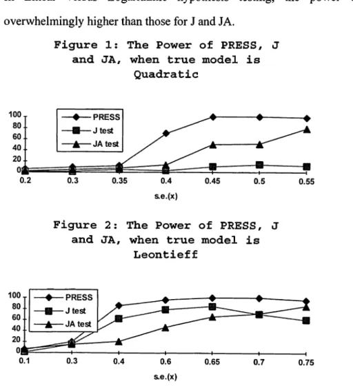
In the power plots, we see a clear superiority o f predictive residual sum o f squares method over J and JA tests.
When the standard error o f the X variable is reduced, the performance o f all tests become closer. But when the standard error o f the x variable is increased the power o f PRESS increases significantly, while the power o f J and JA tests are not as high as the power o f PRESS.
In Quadratic versus Leontieff hypothesis testing, at high standard error o f x variable, the power of JA is higher than J, where both are lower than that o f PRESS. In Linear versus Logarithmic hypothesis testing, the power o f PRESS is overwhelmingly higher than those for J and JA.
Figure 1; The Power of PRESS, J and JA, when true model is
Quadratic
Figure 2; The Power of PRESS, J and JA, when true model is
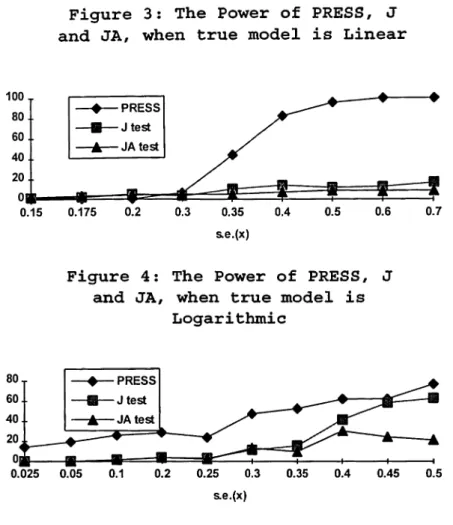
Figure 3: The Power of PRESS, J and JA, when true model is Linear
Figure 4: The Power of PRESS, J and JA, when true model is
Logarithmic
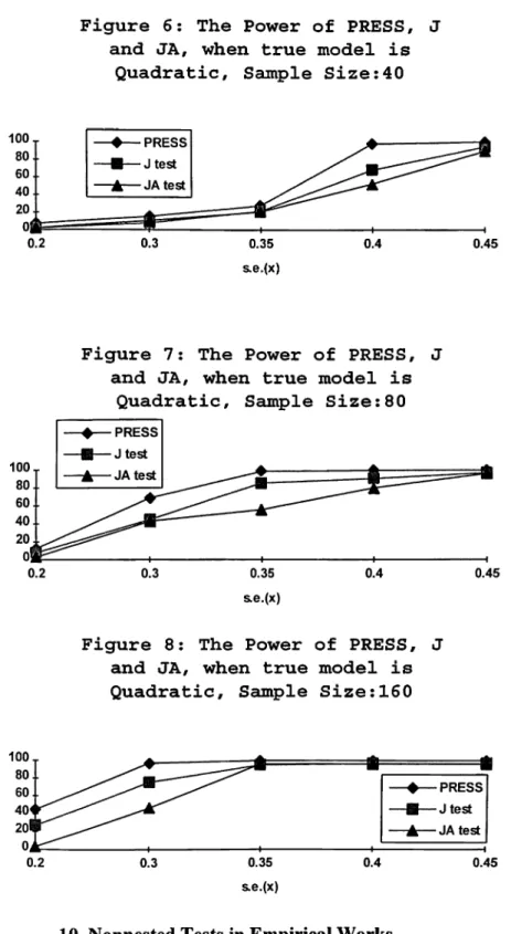
The following four figures show the effect o f increases in sample size on the power o f tests. As the sample size increases the dominance of the PRESS test over J and JA tests is preserved; PRESS still gives the highest power in each different standard error o f the X variable. It can also be observed that as the sample size increases the powers o f all tests increase as each standard error o f X.
Figure 5: The Power of PRESS, J and JA, when true model is
Figure 6; The Power of PRESS, and JA, when true model is
Quadratic, Sample Size:40
Figure 7: The Power of PRESS, and JA, when true model is
Quadratic, Sample Size:80
Figure 8: The Power of PRESS, and JA, when true model is Quadratic, Sample Size:160
10. Nonnested Tests in Empirical Works
Empirical tests on nonnested hypothesis tests are very rare. Basically, nonnested hypothesis tests can be used in identifying model misspecifications. But first, let’s define what a useful model is.
The followings are some conditions set by Hendry and Anderson (1977), Davidson (1978) and Hendry and Ungern-Stemberg (1981) which should be present in a useful model: -data coherency, -data admissibility, -theory consistency, -parameter constancy, -valid conditioning,
-interpretable, parsimonious, orthogonal parameters o f interest, -encompassing contending explanations o f the same phenomena.
In order to satisfy the first five conditions, the orthodox tests for autocorrelation, heteroskedasticity, parameter constancy become model selection criteria. This is because, if a model fails these tests, they are discarded immediately. There is no need for further subjecting the models to nonnested tests to detect a misspecification. Encompassing tests relieves information on how the model approximates the data mechanism. This is because, it may seem difficult to design sensible models to account for all results obtained in previous researches, whereas good approximations should be able to explain contending findings. If all contenders are nested special cases, encompassing is automatic, but if some are separate hypotheses, indirect inference is required, perhaps based on nonnested tests.
Actually, in many practical cases, a specification error that can be detected by a nonnested hypothesis test could also be detected by applying one o f the many orthodox tests available for different types o f model misspecification. Misspecification usually causes heteroskedasticity, serial correlation, failure o f linear or nonlinear restrictions to hold, unstable parameter estimates, correlation between error terms or some other observable misbehavior of the model in consideration. These defects can be detected by classical tests. So in principle, applied econometricians may rarely need nonnested hypothesis tests to detect the above
However, in practice, researchers are very inclined to test their models. Every applied researcher wants to form the best model in order to explain a certain phenomenon. Anything that forces them to tests their model a bit more rigorously is therefore highly desirable. So, when a researcher decides to make use o f nonnested hypothesis tests, he is forced to recognize that there are usually many models around to explain the same phenomenon and that most o f these models must be false. Consequently, he is obliged to estimate several nonnested alternative models, and to give each o f them several chances to show that it is not true by confronting it with the evidence provided by the available data and the other models. Doing this must increase greatly the probability that the model finally selected will not be thoroughly false. If this is the only contribution o f nonnested tests, it will be a very valuable one.
An empirical work in this area is the one done by Pesaran and Deaton (1978). They estimated five models o f consumption behavior and tested them against each other. In this work, the models were deliberately kept very simple for illustrative purposes. Therefore, they can not be taken seriously. They all suffer from numerous econometric problems such that they could easily be rejected by orthodox tests without any further need for noimested hypothesis tests. One o f the serious papers published in this context is the one o f Deaton (1978). In this paper, two competing demand theories were tested against each other. Both models were rejected. Before 1978, some unpublished work exists, but by and large it is fair to say that the literature on nonnested hypothesis testing had no impact whatsoever on empirical works in economics. But since then, this literature is improved by the researches done in Agricultural Economics.
11. Empirical Work: Turkish Consumption Function A. Abstract
The aim o f this section is to examine the consumption behavior in Turkey, by estimating three simple forms o f consumption model: Absolute Income Hypothesis model. Relative Income Hypothesis model and Permanent Income Hypothesis model.
Consumption pattern for the period 1987-1995(2) is considered. Yearly data is taken. During this period, Turkey experienced an unusual pattern of growth. The growth rate o f GDP were very small in years 1988,1989,1991 very large in 1990, 1992, 1993 and 1995 and negative very large in 1994. The high growth rate in population also critically affect the consumption pattern in Turkey. The growth in private consumption over this period was always less than the growth in disposable income, but followed the pattern closely at each year. These suggest that Turkish consumers' behavior fits better to absolute income hypothesis or relative income hypothesis, but Turkish consumers do not have a lifetime pattern of consumption as suggested by Permanent Income hypothesis.
B. Theoretical Framework Absolute Income Hypothesis
This hypothesis is Keynes' contribution to consumption theory. It is a simple observation that consumption increases with income and that marginal propensity to consume is less than 1. At low levels o f income individuals tend to consume a large fraction o f their incomes and at higher income levels, a smaller fraction o f it is consumed cross sectional data is used in this model. The implied model is as follows.
Cf=a + bY(jt, where b is the marginal propensity to consume.
Here, the emphasis is on current disposable income as the principal determinant o f consumption. This function reflects the observation that as income increases people tend to spend a decreasing percentage o f income or conversely tend to save an increasing percentage of income. The behavior o f consumer expenditure in the short-run over the duration of business cycle. Reasoning is that as income falls relative to recent levels, people will protect consumption standards by not cutting consumption proportionally to the drop in income and conversely, as income increases consumption will not rise proportionally.
This is usually taken to mean that the proportion of income consumed, average propensity to consume will tend to fall as income increases.
Any theory o f consumption has to be able to explain the short-run behavior o f consumption. In other words, it has to show the average propensity to consume behaving in a contra cyclical manner over time, cross-sectional data, which shows that at any point in time higher income earners have a lower average propensity to consume than low-income earners and finally, the long-run constancy of the average propensity to consume. It has been felt by economists as early as 1950's that simple Keynesian function had been tested against the available evidence and had been found wanting. Therefore, the search for new theories began and it is to those we now turn.
Relative Income Hypothesis
Duesenberry's relative income hypothesis assumes that consumption is influenced by the consumer's relative income; both current income relative to previous income and current income relative other people's income. So, Duesenberry suggests that consumers' preferences are interdependent. The utility a consumer derives from a given bundle o f consumer goods depends to some extent on what others around him are consuming. In this theory consumption is influenced by the "demonstration effect" of other people's consumption. This assumption leads to the result that the individual's average propensity to consume will depend on his position in income distribution.
A person with income below the average will tend to have a high average propensity to consume, because, essentially, he is trying to keep up to the national average consumption standard with a below-average income. On the other hand, an individual with an above-average income will have a lower average propensity to consume, because it takes a smaller proportion o f his income to buy the standard basket o f consumer goods.
This provides an explanation to the short-run behavior consumption and the long-run constancy o f average propensity to consume. As people learn more about the trend, they can increase their consumption proportionately to maintain the same ratio between their consumption and the national average
This hypothesis suggests that consumption behavior depends on the ratio o f current income to the previous peak level o f income, over the business cycle, along with the current level o f disposable income.
It is more difficult, he argues, for a family to reduce a level o f consumption once attained than to reduce the portion o f its income saved in any period. Actually, the shortcoming o f this hypothesis arises from this assumption. It is the asymmetry suggesting that a current increase in income if it exceeds a previous peak, induces a new consumption standard immediately. Algebraically, Duesenberry's formulation is as follows:
Ct= a + bYdt + dY(jt-i
Permanent Income Hypothesis
Another approach to the consumption function is the permanent income hypothesis, developed by Friedman in mid 1950's. This hypothesis is similar to Duesenberry's hypothesis in that both o f them provides the basis for a consumption function which is not based merely on current income.
The basic notion underlying this hypothesis is permanent income, which is the income generated by the individual's total wealth. Moreover, it is the level o f income that can be expected to persist in the long-run. Over the long-run, there are episodes of positive transitory income and episodes o f negative transitory income, which average out to zero. This hypothesis suggests that the consumption is proportional to permanent income. Friedman further assumes that there is no relationship between the transitory consumption and transitory income.
So, Cp=kYp
Y=Yp+Ytr
C=Cp+Ctr
Cov(Yp,Ytr)=0 Cov(Cp,Cp-)=0According to Friedman, in booms more people will think that they are better than normal than will think they are doing worse than normal. For the economy as a whole, therefore, there will be positive transitory income. Unexpectedly, high income will have little impact on consumer views o f their permanent income unless it lasts for several years. So, unexpected increases in income are therefore largely saved with the result that in boom, the average propensity to consume falls.
It can be seen Friedman is able to explain why the short-run consumption function is flatter with a variable average propensity to consume, while the long-run consumption function is steeper with a constant average propensity to consume. Booms usually cause average propensity to consume to fall.
To be operational, the permanent income hypothesis consumption function requires some means o f measuring permanent income. A common procedure for this is to assume that permanent income is an average of past income with the most recent past weighted most heavily.
This simplification o f Friedman's consumption function is made by Koyck. His methodology is as follows:
Yp-Ydt+eYdt-l+e2Ydt-2+-+e”Ydtn
C^=kYp, so,
Ct=kdenYt_n
eCj.
1
=kde^ Y 1, thenCt-eCt_i=kYt
Ct=kYt+eCt_i
C. Empirical Estimation
Each o f the models considered are first subjected to a series o f tests. These include tests for outliers, normality of errors, non linearity o f regressors, structural stability and heteroskedasticity. Lets briefly discuss the results o f these tests for each model.
Keynes’ Model
The regression result is as follows:
Variable Estimate t-value RSS F
Const. 561.836 17.607 0.988 972.697 3629.681
Ydt
0.57 60.246No outliers is found in this model. So, we do not need to revise our observations. Skewness and Kurtosis are found to be -3258 and 177190 respectively. Both are smaller than 5% critical values, which are 11823 and 1155699 respectively. The model is then tested for possible non linearity. DW statistic is 2.956, but this statistic just tests for first order serial correlation, so another test is implemented. An F test is conducted on the coefficients o f non-linear terms added to the model (Y^t^). F statistic o f this test is extremely small, 0.000276. this test yields that the data do not have any non-linear characteristic. Besides the t-statistic o f Y¿t^ is very small, leading to the same conclusion.
Structural stability is tested using Chow test. F-statistic associated with this test is 0.119, which leads to the conclusion that the structure o f this model is stable. Then the model is tested for the presence o f heteroskedasticity. White test is used in order to do that. The F-statistic o f this test is 2.718 w ith p-value 0.143. So, it can be concluded that asymptotically no heteroskedasticity is present. At least, OLS standard errors and the statistics are valid.
The above regression results show that the constant term is significant. The short-run marginal propensity to consume, which equals to long-run marginal propensity to consume in this model is 0.57.
Duesenberry's Model
The regression results are as follows:
SS F
Z8.748 1629.331 Variable Estimate t-value r2
Const. 559.976 16.538 0.998
No outliers are present for this model as well. Skewness and Kurtosis associated with this model are both smaller than the 5% critical values (1877<11997; 197700<1070896 respectively). So, the errors in this model are normal as well. The OLS statistics are valid. DW statistic is 3.006. When the model is tested for non linearity, the data do not show any evidence of non linearity. The t-statistics associated with the nonlinear terms (Ydt^^Ydt-l^’^ d t^ d t- l) added to the model are all insignificant. Besides the related F-statistic is 0.0522, which is not significant at all. So, we can conclude that data show no non linearity.
Structural stability is tested again by Chow test. The associated F-statistic is 0.575. So, the structure o f this model is stable as well. Then, using White test, this model is tested for heteroskedasticity. The t-statistics o f all terms in this test are very small. Besides, the over all F-statistic is 1.119. All of these findings suggest that heteroskedasticity is not present in the data. With this result o f White test, one can conclude that OLS standard errors and test statistics are valid and can be safely used.
The above regression results show that the constant term is significant. The short-run marginal propensity to consume is 0.56, and the long-run marginal propensity to consume is 0.57, which perfectly suits to the Keynesian model of consumption.
Friedman's model
The regression results are as follows:
Variable Estimate t-value r2 RSS F
Ydt 0.506 5.092 0.951 1117.307 361.028
Ct_i 0.322 2.314
When subjected to least mean square method, we find some outliers present with this model. This is largely due to the omitted constant term in this formulation. The test for normality of errors yields that errors in this model are normal with both Skewness and Kurtosis smaller than 5% critical values ( 92529<1637065;