100 IEEE COMMUNICATIONS LETTERS, VOL. 14, NO. 2, FEBRUARY 2010
Optimal Signaling and Detector Design for Power-Constrained
Binary Communications Systems over Non-Gaussian Channels
C¸a˘grı G¨oken, Student Member, IEEE, Sinan Gezici, Member, IEEE, and Orhan Arikan, Member, IEEE
Abstract—In this letter, joint optimization of signal structuresand detectors is studied for binary communications systems under average power constraints in the presence of additive non-Gaussian noise. First, it is observed that the optimal signal for each symbol can be characterized by a discrete random variable with at most two mass points. Then, optimization over all possible two mass point signals and corresponding maximum
a posteriori probability (MAP) decision rules are considered. It
is shown that the optimization problem can be simplified into an optimization over a number of signal parameters instead of functions, which can be solved via global optimization techniques, such as particle swarm optimization. Finally, the improvements that can be obtained via the joint design of the signaling and the detector are illustrated via an example.
Index Terms—Stochastic signaling, MAP decision rule.
I. INTRODUCTION ANDMOTIVATION
I
N binary communications systems over additive white Gaussian noise channels and under average power con-straints in the form ofE{∣s𝑖∣2} ≤ 𝐴 for 𝑖 = 0, 1, the averageprobability of error is minimized when deterministic antipodal signals (s0= −s1) are used at the power limit (∣s0∣2= ∣s1∣2=
𝐴) and a maximum a posteriori probability (MAP) decision
rule is employed at the receiver [1]. In addition, when the Gaussian noise is colored, the deterministic antipodal signals along the eigenvector of the covariance matrix of the Gaussian noise corresponding to the minimum eigenvalue minimizes the average probability of error [1]. Although the optimal detector and signaling techniques are well-known when the noise is Gaussian, the noise can have significantly different probability distribution from the Gaussian distribution in some cases due to effects such as interference and jamming [2]. In the presence of non-Gaussian noise, stochastic signaling, which models signals s0 and s1 as random variables, can
result in improved probability of error performance compared to deterministic signaling. In [3], optimal stochastic signaling is studied under second and fourth moment constraints for a fixed decision rule (detector) at the receiver, and sufficient conditions are presented to determine whether stochastic sig-naling can provide performance improvements compared to deterministic signaling. In [4], randomization between two deterministic signal pairs and the corresponding MAP decision rules is studied under the assumption that the receiver knows which deterministic signal pair is transmitted. It is shown that power randomization can result in significant performance improvement.
Although optimal stochastic signaling is studied for a fixed detector in [3] and the effects of randomization between two Manuscript received September 18, 2009. The associate editor coordinating the review of this letter and approving it for publication was W. Hamouda.
The authors are with the Dept. of Electrical and Electronics Engineering, Bilkent University, Bilkent, Ankara 06800, Turkey (e-mail:{goken, gezici,
oarikan}@ee.bilkent.edu.tr).
Digital Object Identifier 10.1109/LCOMM.2010.02.091875
signaling approaches are considered in [4], no studies have focused on the joint optimization of stochastic signaling and the decision rule (detector). In this letter, this joint optimiza-tion problem is formulated, which involves optimizaoptimiza-tion over a function space. Then, theoretical results are provided to show that the optimal solution can be obtained by searching over a number of variables instead of functions, which greatly simpli-fies the original formulation. In addition, a global optimization approach, namely particle swarm optimization (PSO) [5], is employed to obtain the optimal signals and the decision rule. The main motivation behind this study is to provide the-oretical performance limits on the error probability of com-munications systems under power constraints. It is assumed that there is a feedback from the receiver to the transmitter so that the joint optimization of the signaling structure and the decision rule can be performed. This scenario is reasonable for cognitive radio systems, and provides theoretical limits on the error performance of other communications systems.
II. OPTIMALSIGNALING ANDDETECTORDESIGN Consider a binary communications system, in which the receiver obtains𝐾-dimensional observations over an additive
noise channel:
y = s𝑖+ n , 𝑖 ∈ {0, 1} , (1)
wherey is the noisy observation, s0ands1represent the
trans-mitted signal values for symbol0 and symbol 1, respectively, and n is the noise component that is independent of s𝑖. In
addition, the prior probabilities of the symbols, represented by𝜋0 and𝜋1, are assumed to be known.
The receiver uses the observation in (1) in order to de-termine the information symbol. A generic decision rule (detector) is considered for that purpose, which estimates the transmitted symbol based on a given observationy as follows:
𝜙(y) =
{
0 , y ∈ Γ𝜙0 1 , y ∈ Γ𝜙1
, (2)
whereΓ𝜙0 andΓ𝜙1 are the decision regions for symbol0 and symbol 1, respectively [1].
The average probability of error for a decision rule 𝜙 can
be expressed asPe = 𝜋0Pe,0+ 𝜋1Pe,1, where
Pe,𝑖=
∫
Γ𝜙1−𝑖𝑝𝑖(y) 𝑑y , (3)
for 𝑖 = 0, 1, represents the probability of error, with 𝑝𝑖(y)
denoting the conditional probability density function (PDF) of the observation, when the 𝑖th symbol is transmitted.
Unlike the conventional case, a stochastic signaling frame-work is adopted in this study [3], and s0 and s1 in (1) are
modeled as random variables. Since the signals and the noise are independent, the conditional PDFs of the observation can 1089-7798/10$25.00 c⃝ 2010 IEEE
G ¨OKEN et al.: OPTIMAL SIGNALING AND DETECTOR DESIGN FOR POWER-CONSTRAINED BINARY COMMUNICATIONS SYSTEMS. . . 101
be calculated as𝑝𝑖(y) =∫ℝ𝐾𝑝s𝑖(x)𝑝n(y−x) 𝑑x for 𝑖 = 0, 1.
Then, after some manipulation, (3) can be expressed as Pe,𝑖= E {∫ Γ𝜙1−𝑖 𝑝n(y − s𝑖) 𝑑y } ≜ E {𝑓(𝜙 ; s𝑖)} , (4)
where the expectation is taken over the PDF ofs𝑖.
In a practical system, there is a constraint on the average power of the signals, which can be expressed as [1]
E{∣s𝑖∣2}≤ 𝐴 , for 𝑖 = 0, 1 , (5)
where𝐴 is the average power limit. Then, the optimal
signal-ing and detector design problem can be stated as min
𝑝s0,𝑝s1,𝜙 𝜋0Pe,0+ 𝜋1Pe,1
subject toE{∣s𝑖∣2}≤ 𝐴 , 𝑖 = 0, 1 , (6)
wherePe,𝑖is as in (4).
The problem in (6) is difficult to solve in general since the optimization needs to be performed over a space of PDFs and decision rules. In the following, a simpler optimization problem over a set of variables (instead of functions) is formulated to obtain optimal signal PDFs and the decision rule. To that aim, the following result is obtained first.
Lemma 1: Assume𝑓(𝜙 ; s𝑖) in (4) is a continuous function
ofs𝑖, and each component ofs𝑖 resides in [−𝛾, 𝛾] for some
finite 𝛾 > 0. Then, for a given (fixed) decision rule 𝜙, the solution of the optimization problem in (6) is in the form of
𝑝s𝑖(y) = 𝜆𝑖𝛿(y − s𝑖1) + (1 − 𝜆𝑖)𝛿(y − s𝑖2) , (7)
for𝑖 = 0, 1, where 𝜆𝑖∈ [0, 1].
Proof: When the decision rule 𝜙 is given, 𝑓(𝜙 ; s𝑖) =
∫
Γ𝜙1−𝑖𝑝n(y − s𝑖) 𝑑y in (4) can be considered as a function
of s𝑖 only. In other words, Pe,𝑖 in (4) can be expressed as
Pe,𝑖 = E{𝑓(s𝑖)} for 𝑖 = 0, 1. Since the objective function
in (6) is the sum of 𝜋0Pe,0 and 𝜋1Pe,1, and the average
power constraints are individually imposed on the signals, the optimization problem in (6) can be decoupled into two separate optimization problems as follows:
min
𝑝s𝑖 E{𝑓(s𝑖)} , subject to E
{
∣s𝑖∣2}≤ 𝐴 , (8)
for𝑖 = 0, 1. Optimization problems in the form of (8) have
been investigated in various studies in the literature [3], [4]. Under the conditions in the lemma, the optimal solution of (8) can be represented by a randomization of at most two signal levels as a result of Carath´eodory’s theorem [6]. Hence, the optimal signal PDFs can be expressed as in (7).□
Lemma 1 states that, under certain conditions, the optimal stochastic signaling involves randomization among at most four different signal levels (two for symbol “0” and two for symbol “1”). Therefore, the problem in (6) can be solved over the signal PDFs that are in the form of (7). Hence, the search space for the optimization problem is reduced significantly. To achieve further simplification, the following result is obtained. Proposition 1: Under the conditions in Lemma 1, the
optimization problem in (6) can be expressed as follows:
min
{𝜆𝑖,s𝑖1,s𝑖2}1𝑖=0
∫
ℝ𝐾min{𝜋0𝑔0(y) , 𝜋1𝑔1(y)} 𝑑y
subject to 𝜆𝑖∣s𝑖1∣2+ (1 − 𝜆𝑖)∣s𝑖2∣2≤ 𝐴
𝜆𝑖∈ [0, 1] , 𝑖 = 0, 1 (9)
where𝑔𝑖(y) = 𝜆𝑖𝑝n(y − s𝑖1) + (1 − 𝜆𝑖)𝑝n(y − s𝑖2).
Proof: For a given signal PDF pair𝑝s0 and𝑝s1, the condi-tional probability of observationy in (1) can be expressed as
𝑝𝑖(y) =∫ℝ𝐾𝑝s𝑖(x)𝑝n(y − x)𝑑x for 𝑖 = 0, 1. When deciding
between two symbols based on observationy, the MAP deci-sion rule, which selects symbol 1 if 𝜋1𝑝1(y) ≥ 𝜋0𝑝0(y) and
selects symbol0 otherwise, minimizes the average probability of error [1]. Therefore, when signal PDFs 𝑝s0 and 𝑝s1 are specified, it is not necessary to search over all the decision rules; only the MAP decision rule should be determined and its corresponding average probability of error should be considered.
From (3), the average probability of error for any decision rule 𝜙 can be expressed as
Pe=
∫
Γ𝜙1𝜋0𝑝0(y) 𝑑y +
∫
Γ𝜙0𝜋1𝑝1(y) 𝑑y . (10)
Since the MAP decision rule decides symbol1 if 𝜋1𝑝1(y) ≥
𝜋0𝑝0(y) and decides symbol 0 otherwise, the average
proba-bility of error expression in (10) can be expressed for a MAP decision rule as [7]
Pe=
∫
ℝ𝐾min {𝜋0𝑝0(y) , 𝜋1𝑝1(y)} 𝑑y . (11)
Since Lemma 1 states that the optimal signal PDFs are in the form of (7), the conditional PDFs𝑝𝑖(y) =∫ℝ𝐾𝑝s𝑖(x)𝑝n(y −
x)𝑑x can be obtained as 𝑝𝑖(y) = 𝜆𝑖𝑝n(y − s𝑖1) + (1 −
𝜆𝑖)𝑝n(y − s𝑖2), and the average power constraints in (6)
become𝜆𝑖∣s𝑖1∣2+ (1 − 𝜆𝑖)∣s𝑖2∣2≤ 𝐴, for 𝑖 = 0, 1. Therefore,
(11) implies that the optimization problem in (6) can be implemented as the constrained minimization problem in the proposition.□
Comparison of the optimization problems in (6) and (9) reveals that the latter is much simpler than the former since it is over a set of variables instead of a set of functions. However, it is still a non-convex optimization problem in general; hence, global optimization techniques, such as PSO, differential evo-lution and genetic algorithms, should be employed to obtain the optimal PDF [5]. In this letter, the PSO approach is used in the next section to obtain the solution of (9).
After obtaining the solution of the optimization problem in (9), the optimal signals are specified as𝑝opt
s𝑖 (y) = 𝜆opt𝑖 𝛿(y −
sopt𝑖1 ) + (1 − 𝜆opt𝑖 )𝛿(y − sopt𝑖2 ) for 𝑖 = 0, 1, and the optimal detector becomes the MAP decision rule that decides symbol 1 if 𝜋1𝑝opts1 (y) ≥ 𝜋0𝑝opts0(y) and decides symbol 0 otherwise. Finally, it should be noted for symmetric signaling, that is, whens01= −s11,s02= −s12 and𝜆0= 𝜆1, the optimization
in (9) can be performed overs11,s12 and𝜆1 only.
III. NUMERICALRESULTS ANDCONCLUSIONS A numerical example is presented to illustrate the improve-ments that can be obtained via the joint design of the signaling structure and the decision rule for scalar observations. The
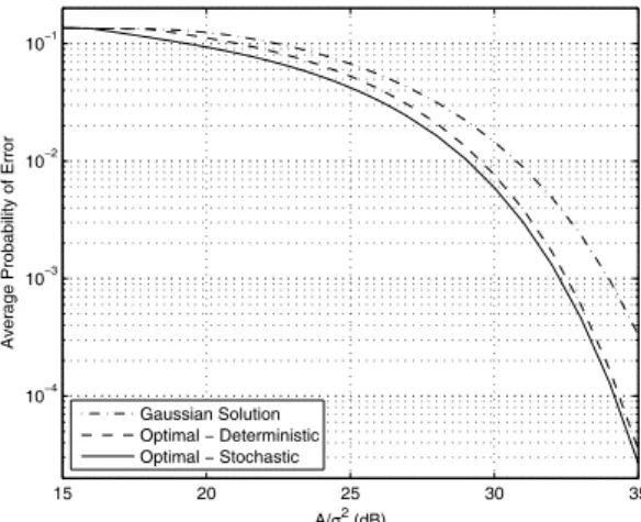
102 IEEE COMMUNICATIONS LETTERS, VOL. 14, NO. 2, FEBRUARY 2010 15 20 25 30 35 10−4 10−3 10−2 10−1 A/σ2 (dB)
Average Probability of Error
Gaussian Solution Optimal − Deterministic Optimal − Stochastic
Fig. 1. Average probability of error versus𝐴/𝜎2 for the three algorithms. noise in (1) is modeled by a Gaussian mixture as in [2] with its PDF being given by𝑝𝑛(𝑦) = √2𝜋 𝜎𝐿1 ∑𝐿𝑖=1e−(𝑦−𝝁𝑖)22𝜎2 , where
𝐿 = 6 and 𝝁 = [0.27 0.81 1.08 − 1.08 − 0.81 − 0.27]
are used. Note that the average power of the noise can be calculated asE{𝑛2} = 𝜎2+ 0.6318. In addition, the average
power limit in (5) is set to𝐴 = 1 and equally likely symbols
are considered (𝜋0= 𝜋1= 0.5).
In the following, three different approaches are compared. Gaussian Solution: In this case, the transmitter is assumed to have no information about the noise PDF and selects the signals ass0= −√𝐴 and s1=√𝐴 , which are known to be
optimal in the presence of zero-mean Gaussian noise [1]. On the other hand, the MAP decision rule is used at the receiver. Optimal – Stochastic: This approach refers to the solution of the most generic optimization problem in (6), which can also be obtained from (9) as studied in the previous section.
Optimal – Deterministic: This is a simplified version of the optimal solution in (9). It assumes that the signals are deterministic; i.e., they are not randomization of two different signal levels. Hence, the optimization problem in (9) becomes
min
s0,s1
∫
ℝ𝐾min{𝜋0𝑝n(y − s0) , 𝜋1𝑝n(y − s1)} 𝑑y
subject to ∣s0∣2≤ 𝐴 , ∣s1∣2≤ 𝐴 . (12)
In other words, this approach provides the optimal solution when the signals are deterministic.
In Fig. 1, the average probabilities of error are plotted versus
𝐴/𝜎2for the three algorithms above by considering symmetric
signaling. In obtaining the optimal stochastic solution from (9), the PSO algorithm is employed with 50 particles and 1000 iterations. Please refer to [5] for the details of the PSO algorithm1. On the other hand, the optimal deterministic
solution in (12) can be obtained via a one-dimensional search due to symmetric signaling. From Fig. 1, it is observed that the Gaussian solution performs significantly worse than the optimal approaches for small 𝜎 values. In addition, the
optimal approach based on stochastic signaling has the best performance.
In order to explain the results in Fig. 1, Table I presents the solutions of the optimization problems in (6) and (12) for the optimal stochastic and the optimal deterministic approaches,
1The other parameters are set to𝑐
1= 𝑐2= 2.05 and 𝜒 = 0.72984, and the inertia weight𝜔 is changed from 1.2 to 0.1 linearly with the iteration
number [5].
TABLE I
OPTIMAL STOCHASTIC AND DETERMINISTIC SIGNALS FOR SYMBOL1.
Stochastic Deterministic 𝐴/𝜎2 (dB) 𝜆 1 s11 s12 s1 15 N/A 1 1 1 20 0.1836 1.648 0.7846 0.7927 25 0.2104 1.614 0.7576 0.7587 30 0.2260 1.586 0.7475 0.7476 35 0.2347 1.568 0.7441 0.8759
respectively. Note that the results for symbol 1 are listed in Table I, and the results for symbol 0 are the negatives of the signal values in the table since symmetric signaling is considered. For small 𝐴/𝜎2 values, such as 15 dB, the
optimal solutions are the same as the Gaussian solution, that is, s11 = s12 = s1 = √𝐴 = 1. However, for large 𝐴/𝜎2’s,
the Gaussian solution becomes quite suboptimal and choosing the largest possible deterministic signal value, 1, results in higher average probabilities of error, as can be observed from Fig. 1. For example, at 𝐴/𝜎2 = 30 dB, the optimal
deterministic solution sets s1 = −s0 = 0.7476 and achieves
an error rate of 7.66 × 10⁻³, whereas the Gaussian one uses
s1 = −s0 = 1, which yields an error rate of 0.0146. This
seemingly counterintuitive result is obtained since the average probability of error is related to the area under the overlaps of the two shifted noise PDFs as in (12). Although optimal deterministic signaling uses less power than permitted, it results in a lower error probability than Gaussian signaling by avoiding the overlaps between the components of the Gaussian mixture noise more effectively. On the other hand, optimal stochastic signaling further reduces the average probability of error by using all the available power and assigning some of the power to a large signal component that results in less overlapping between the shifted noise PDFs. For example, at
𝐴/𝜎2= 30 dB, the optimal stochastic signal is a
randomiza-tion ofs11 = −s01 = 1.586 and s12 = −s02= 0.7475 with
𝜆0 = 𝜆1 = 0.226 (cf. (7)), which achieves an error rate of
5.95 × 10⁻³.
The results in this letter can be extended to 𝑀-ary
com-munications systems as well by noting that the average probability of error expression in (11) becomes Pe = 1 −
∫
max{𝜋0𝑝0(y), . . . , 𝜋𝑀−1𝑝𝑀−1(y)}𝑑y for 𝑀-ary systems.
Then, an optimization problem similar to that in Proposition 1 can be obtained, where the optimization is performed over
{𝜆𝑖, s𝑖1, s𝑖2}𝑀−1𝑖=0 .
REFERENCES
[1] H. V. Poor, An Introduction to Signal Detection and Estimation, 2nd ed., New York: Springer-Verlag, 1994.
[2] V. Bhatia and B. Mulgrew, “Non-parametric likelihood based channel estimator for Gaussian mixture noise,” Signal Processing, vol. 87, pp. 2569–2586, Nov. 2007.
[3] C. Goken, S. Gezici, and O. Arikan, “Stochastic signaling under sec-ond and fourth moment constraints,” submitted, Jan. 2010. [Available: www.ee.bilkent.edu.tr/∼gezici/goken.pdf].
[4] A. Patel and B. Kosko, “Optimal noise benefits in Neyman-Pearson and inequality-constrained signal detection,” IEEE Trans. Sig. Processing, vol. 57, no. 5, pp. 1655–1669, May 2009.
[5] K. E. Parsopoulos and M. N. Vrahatis, Particle swarm optimization
method for constrained optimization problems. IOS Press, 2002, pp.
214–220, in Intelligent Technologies–Theory and Applications: New Trends in Intelligent Technologies.
[6] R. T. Rockafellar and R. J.-B. Wets, Variational Analysis, Berlin: Springer-Verlag, 2004.
[7] M. Azizoglu, “Convexity properties in binary detection problems,” IEEE