Sustainability of the Actuarial Balance: Turkey’s Experience Between 1972-2013

(1)

Doğuş Üniversitesi Dergisi, 20 (1) 2019, 141-158

(1)_{Türkiye İş Kurumu Genel Müdürlüğü, yasar.yasarlar@iskur.gov.tr} (2)_{İstanbul Üniversitesi, İktisat Bölümü, ybayraktar@istanbul.edu.tr} Geliş/Received: 25-04-2018, Kabul/Accepted: 13-12-2018

Sustainability of the Actuarial Balance: Turkey’s Experience

Between 1972-2013

1

Aktüeryal Dengenin Sürdürülebilirliği: 1972-2013 Arası Türkiye Deneyimi

Yaşar YAŞARLAR (1)_{, Yüksel BAYRAKTAR}(2)

ABSTRACT: This study is designed based on a two-part hypothesis that (1) active/passive ratios, which are the most commonly used criteria in measuring financial balances of social security institutions in Turkey, are a good indicator and that (2) the 1972-2013 actuarial balance is not sustainable. In this study, demographic, economic, and several other factors thought to affect the actuarial balance in Turkey were analysed using multiple regression, the Johansen Cointegration Test, ECM, and VECM. The results of the analyses revealed the short- and long-run effects of the said factors on the actuarial balance sustainability. The results also proved that the active/passive ratios were a good indicator and the actuarial balance between 1972 and 2013 in Turkey was not sustainable.

Keywords: Actuarial Balance, Sustainability, Turkish Pension System, Social Security Institution

ÖZ: Bu çalışma, Türkiye özelinde sosyal güvenlik kurumlarının finansal dengelerinin

ölçülmesinde en yaygın şekilde kullanılan kriter olan aktif/pasif oranlarının (1) iyi bir gösterge olduğu ve (2) 1972-2013 dönemi için aktüeryal dengenin sürdürülebilir olmadığı şeklindeki iki parçalı hipotez üzerine şekillenmiştir. Bu çalışmada, Türkiye için aktüeryal dengenin sürdürülebilirliği etkilediği düşünülen demografik, ekonomik ve diğer faktörler; çoklu regresyon, Johansen Eşbütünleşme, ECM ve VECM ile analiz edilmiştir. Analizlerin bulguları bu faktörlerin kısa ve uzun vadede aktüeryal dengenin sürdürülebilirliğine etkilerini ortaya çıkarmıştır. Ayrıca söz konusu bulgular aktif/pasif oranlarının iyi bir gösterge olduğu ve çalışma kapsamında 1972-2013 dönemi için Türkiye’de aktüeryal dengenin sürdürülebilir olmadığı ispatlamıştır.

Anahtar Kelimeler: Aktüeryal Denge, Sürdürülebilirlik, Türk Sosyal Güvenlik

Sistemi, Sosyal Sigortalar Kurumu

Jel Classifications: C01, G22, H55

1. Introduction

Actuarial balance involves insurance companies meeting damage payments by the insurance products created for risks transferred to these companies and premiums received in exchange for these products. The fundamental point here is that the contributions made are equivalent to benefits procured (Tuna, 2009). The US Congressional Budget Office defines actuarial balance as the difference between

1_{This paper is based on Yaşarlar (2016) PhD. study titled ‘Sustainability of actuarial} balance: Experience of Turkey’.

(2)

142 Yaşar YAŞARLAR, Yüksel BAYRAKTAR

social security income and cost ratios (Congress of The United States, 2013). According to Social Security Institution (SGK), social security institution in Turkey, actuarial balance is the ability to compensate expenses using both the income collected and excess reserves (Tuna, 2009). While in a narrower sense, actuarial sustainability refers to whether a pension system will be able to continue providing benefits in a sustainable manner in the future; actuarial sustainability may be more broadly understood as comprising the non-monetary aspects of systemic stability related to distributive justice (Mattil, 2006).

Three different models were constructed during the present study examining the sustainability of Turkey’s 1972-2013 actuarial balance; using namely, a multiple regression model, a cointegration analysis model, and a vector error correction model. The specific aim of this study is to test, within a Turkish context, sustainability of the actuarial balance between 1972 and 2013 by taking active/passive ratios as its basis, as they are the most commonly used criteria in measuring financial balances of social security institutions.

2. Literature

Although the primary literature pertaining to the measurement of the actuarial balance sustainability began to accumulate in the 1990s, the US Board of Trustees of the Federal OASI and Disability Insurance Trust Funds has prepared a report analysing sustainability of the actuarial balance every year since 1941 (Boado-Penas and Vidal-Meliá, 2013). In the field’s pioneering study, Lee and Tuljapurkar (1998) used an ARIMA model including time series data on fertility, death, productivity, and interest rates for the USA between 1948 and 1994 in order to make predictions for trust funds for the years 1995-2007. According to these predictions, if the taxation and benefit rates in the current pension system fail to change, there is a 95% probability that pension funds will be exhausted from 2014 to 2037 and a 2.5% probability that pension funds will be balanced in 2070. If the social security tax rate is immediately increased by 1%, there is a 92% probability that these funds will be exhausted before 2070, while an increase of between 2-2.19% makes for a 75% probability of such funds to be exhausted by the same year. In addition, the results of the Chow test performed to detect structural breaks revealed that the data collected both prior to and post 1961 did not experience a significant change. Results of the study also revealed that fertility rate was the greatest source of ambiguity in the pension system’s long-run financing, and that death rate was the least significant variable.

Plamondon et al. (2002), whose study was later published in a book form by the ILO, used a multiple regression analysis with demographic data (fertility, death, migration, and dependency rates) and economic data (labour force participation, employment, unemployment, GNP growth, inflation, wage growth, and interest rates) for the small Caribbean island of Guyana between 1998-2000 to make predictions between 2000-2050. Their results revealed that the National Insurance Programme’s financial state was actuarially healthy and that the cost of retirement insurance will increase in stages over the next ten years thereby requiring an increase in contribution rates, recommending that certain rules be implemented in order to determine financing goals and to guide contribution rates increases.

Improving on the data set and analysis method used in Lee and Tuljapurkar’s (1998) study, Lee, Anderson and Tuljapurkar. (2003: 1-17) used US data from 1940 to 2001

(3)

Sustainability of the Actuarial Balance: Turkey’s Experience Between 1972-2013

143

to make predictions on trust funds for 2002-2077. The authors first conducted a multiple regression analysis using the following data based on gender and age: (i) social security taxes paid per-capita and social security benefits, (ii) the number of individuals in the system, (iii) administration expenses belonging to the pension system, (iv) total taxes collected, (v) total social security benefits, and (vi) the total taxed rate of retirement and disability wages. The authors then used a VAR model into which they entered the real wage increase rate, the real interest rate, and return on equity data in order to make their predictions. A low level correlation was found among the variables in the VAR analysis. The results of their study revealed that (i) although the fund’s actuarial balance is predicted to remain positive until 2041, there is a 50% probability of insolvency by 2038, (ii) assuming a 50% solvency probability until the year 2014, the fund’s actuarial balance is expected to remain positive until 2047 by raising the retirement age to 69 beginning in 2024, and (iii) assuming a 50% solvency probability until the year 2077, the fund’s actuarial balance is expected to remain positive until 2101 by raising payroll tax by 1%, increasing the age of retirement to 69, and investing 25% of the fund in equities.

Roach and Ackerman (2005: 10-29) performed a multiple regression analysis using average yearly per-capita income, taxable income time series data for the USA between 1990 and 2003 to make predictions for trust funds. In their study, in order for actuarial balance to be sustainable in 2080, three political actions were recommended to be implemented: (i) taxes collected from wages needed to be increased by 0.5% every year until 2017, reaching a total increase of 6% while also reducing social security benefits by a total of 16%, (ii) social security tax rates needed to be increased by 0.1% every year until 2013, reaching a total increase of 0.7%, and (iii) social security tax needed to be immediately increased by 0.4%.

Boado-Penas, Sakamato and Vidal Meliá (2009: 5, 8) used a financial statement evaluation model (Swedish model) into which they entered actuarial income and expense monthly time series data for Sweden between 2004 and 2008 to make predictions for 2008-2082. Aiming to balance the actuarial imbalance in the Swedish pension system, a law was passed regarding Automatic Balancing Mechanisms (ABM) (Boado-Penas and Vidal Meliá, 2013). When solvency ratio (total income divided by total expenses) falls below 1, ABMs come into force to quickly resolve this imbalance. According to the 75-year prediction made in 2007, while solvency rate will be 1.1 in 2037 in the best case scenario, it will fall below 1.0 in 2025 in the worst case scenario (Boado-Penas, Sakamato and Vidal Meliá, 2009: 8).

The first study in the literature on this subject examining Turkey was that of Sayan (2005: 37-53), in which he used the genetic algorithm method to examine the different combinations of premium rate, income replacement rate, and retirement age which will minimise today’s discounted real value of accumulated deficit created by SSK’s (Social Insurance Institution) old age insurance operation between 2000 and 2060 (A). The study exhibited the expected results of the 1999 and 2002 regulations on SSK’s income-expense balances concerning retirement age until the year 2060. By virtue of the 1999 reforms, it was predicted that SSK’s -300 trillion ₺ deficit in 2000 would fall to -200 trillion ₺ in 2060. Following the 2002 intervention into SSK’s deficit, it was predicted that the deficit would fall to -100 trillion ₺ in 2020. Had these regulations not been made, it was predicted that the SSK deficit would reach -850 trillion ₺ in 2060.

(4)

In his study in which he developed a model based on the effects that replacement rate and contribution rate, both concepts treated in Sayan and Turhan-Sayan’s (2001) yet to be published article, have on labour and retirement income flexibility of labour force, Alparslan (2005) used the genetic algorithm method in order to discuss a realistic model for parametric pension reform alternatives. The study predicted two scenarios concerning SSK’s accumulated deficit based on the 1999, 2002, and (expected) 2006 reforms. In the first scenario, in addition to the total actuarial deficit being zero, the model horizon would not only produce higher actuarial surpluses than in previous years, it would also allow for a lower replacement rate/contribution rate rationing than the current situation. In the second scenario, not only would the total actuarial deficit be near zero, the high actuarial surpluses produced in previous years would also continue. It is also observed in this second scenario that the actuarial deficit would increase as a result of important changes in the number of retired individuals.

Keskin (2006) conducted an ANOVA analysis using SSK data for maximum and minimum premium based earnings as well as the average value from 1978 to 2006 in order to make predictions regarding social security deficits under a variety of demographic projections for 2007-2095. Keskin adds three more scenarios to Sayan’s three predictions concerning legal processes. According to Keskin’s first scenario, SSK’s 100 trillion ₺ deficit in 2005 will shrink to 60 trillion ₺ in 2095. Keskin’s second scenario predicts that the SSK deficit will shrink to approximately 30 trillion ₺ in 2095 whereas in her third scenario, the SSK deficit will be reduced to zero by 2095.

Akyıldız and Yavuz (2007: 424-436) conducted a multiple regression analysis in order to measure effects active/passive ratios and real pension data belonging to SSK, Bagkur (Artisans and Craftsmen and Other Independent Workers Social Security Institution), and Emekli Sandığı (State Employees’ Pension Fund) on the financial deficits of these social security institutions for the years 1989-2006. The results of the study revealed that SSK’s actuarial balance would improve. Moreover, while no significant relation was found between SSK’s actuarial and financing balance, one was found for both Emekli Sandığı and Bagkur.

Ündemir (2009) conducted a stationary analysis on SGK’s 4/a (SSK), 4/b (Bagkur), and 4/c (Emekli Sandığı) items from 1972 to 2008, making predictions for actively insured individuals, passively insured individuals, and covered population series for 2009-2023. While predictions for actively insured individuals of 4/b and its covered population series, and 4/c’s covered population series was made via Winters exponential smoothing method, Holt exponential smoothing method was used to make predictions for all the other series. According to the analyses conducted in the study, no change was predicted in active/passive ratio for 4/a. However, it was predicted that the 2009 active/passive ratio of 1.92 for 4/b and active/passive ratio of 1.51 for 4/c would fall to 1.41 and 1.31, respectively, in 2023.

Güner (2012) developed seven multi-regression based models containing SGK data from 1990 to 2010, the results of which revealed that active-passive ratios significantly affected the financing system. For this reason, the need to prevent informal employment and frequent applications to premium amnesty laws, as well as the need to take other preventive measures, were revealed. Güner’s study contributed to the literature by using of a new set of data and by revealing theoretic relationships through the use of seven separate models.

(5)

145

3. Data and Methodology

The most commonly used criteria in measuring financial balances of premium-based social security instutions are the active/passive ratios. These ratios express how many employees (actively insured individuals) balance out retired individuals and/or dependents (passively insured individuals) in a pension system (Acar and Kitapcı, 2008: 80). Today, while six employees finance one retired individual in OECD countries and four employees finance one retired individual in EU countries, approximately two employees finance one retired individual in Turkey. In 2014, SGK’s active/passive ratio was 1.94 (SGK, 2015) which below the signal level of 2 necessary to sustain the actuarial balance (Acar and Kitapcı, 2008: 80). This is due to Turkey having such a high number of retired individuals. That is, compared to EU countries, there are more retired individuals needing to be financed. As a result, the “necessary condition” in order to sustain the actuarial balance is an active/passive ratio of at least 2 whereas a ratio of at least 4 may be considered a “sufficient condition.” When the necessary condition is fulfilled, the actuarial balance is considered to be “sustainable at a weak level” whereas if the sufficient condition is met, it is considered to be “sustainable at a strong level.”

Sustainability of the actuarial balance generally consists of empirical studies of time series analyses based on a multiple linear regression model and/or VAR model analyses whose independent variables consist of demographic data (such as fertility, death, migration, dependency rates) and economic data (such as labour force participation, employment, unemployment, GDP growth, inflation, wage growth, interest rates), and dependent variable is the actuarial balance. Our study is divided into three stages. In the first stage, an actuarial balance model will be constructed using a time series analysis approach based on a multiple-linear regression model of the dependent variable (active/passive ratios). In the second stage of the analysis, a Johansen Cointegration Test and an ECM will be conducted to determine the model’s long- and short-run effects, respectively, on the actuarial balance variability. In the third and final stage, a VEC model will be constructed, impulse-response and variance decomposition analyses will be conducted, and future predictions will be made, thereby concluding the study.

Law number 1479, coming into force 02 Oct 1971, established the social security institution for Artisans and Craftsmen and Other Independent Workers Social Security Institution (Bagkur), the latest established Institution of the former system. Beginning from 1972 when Bagkur released its first balance sheet, this system was run under three separate social security bodies (i) the State Employees’ Pension Fund, (ii) the Social Insurance Institution, and (iii) Bagkur until 2007, at which time they were brought under a single administrative roof called the Social Security Institution (SGK) by law number 5510, otherwise known as the “Social Insurance and Universal Health Insurance Law,” that came into force in 2008. Variables of this study consist of data from 1972 to 2007 collected from the former system’s three separate bodies as well as SGK data for the active/passive ratio (ACTPASS) which will be the dependent variable, income/expense ratio (INCEXP), and insured population/total population of Turkey ratio (COVER) from 2008 to 2013 collected from the latter system. The demographic data included in this study consist of OECD data for Turkey’s fertility rate (FERT) and death rate (DEATH) whereas macro-economic data consist of TURKSTAT data for the inflation rate (INF) and interest rate (INT). Data for GDP

(6)

growth rate (GDP) consist of data from Republic of Turkey Ministry of Development for the years 1972-1997 and data from TURKSTAT for the years 1988-2013. Data on the unemployment rate (UNEM) for individuals aged 15+ consist of data from TURKSTAT for the years 1989-2013 and for the years 1972-1988, from Tuncer Bulutay, who collected and consolidated data from TURKSTAT’s predecessor organisation, SSI (Bulutay, 1995). Data sets contain data from 1972-2013. A graphic examination was performed on the series and disproportional series’ (ACTPASS, GDP, and FERT) logarithmic conversion were performed. An “L” was placed at the beginning of those variables that underwent logarithmic conversion. First of all, Model-1 of multiple regression will be contracted with all these variables included. The equation of Model-1 is shown below:

0 1 5 6 7 8 2 3 8 4 t t t t t t t t t t

D( L _ ACTPASS) D(L _ GDP) D(L _ FERT) D( INT ) D(INCEX ) D(UNEM ) D( COVER ) D( DEATH ) D( INF ) (TREN

P D )                       (1)

The second multiple regression model, Model-2 İS constructed after the insignificant variables are removed from Model-1 via using the general-to-specific method. The equation of Model-2 is as follows:

0 1 t 2 3 4

t t t t

) D( ) D(

D( L _ ACTPASS    L_ FERT  INCEXP)D( COVER)(TREND) (2)

Cointegration analyses provide the opportunity to test the stationary of non-stationary series’ linear combinations and in the case that stationary are determined, the opportunity to examine their long-run balance dynamics. In addition to this, cointegration analyses are based on the assumption that although series may not be stationary, a long-run relationship may still exist between them and this relationship may have a stationary structure. (Tarı and Yıldırım, 2006: 100). The critical values used in the tests were indicated by Johansen and Juselius (1990: 208, 209) and by Osterwald-Lenum (1992: 467-472). When all of these are considered, a Johansen Cointegration Analysis will be implemented in this study and the equation that will be used in this Analysis is given below:

0 1 t 2 3

t t t t

( L _ ACTPASS

)



 



(

L _ FERT

)





(

INCEXP

)





( COVER )





(3) According to Granger’s Representation Theorem (Engle and Granger, 1987: 251, 252), if two variables are cointegrated there exists a long-run relationship between them. The short-run imbalance occurring between these two variables is corrected using the error correction mechanism. In order for the error correction mechanism to work, it is necessary that the ECT(-1) coefficient, in other words adjustment coefficient be between -1 and 0 (Sevüktekin and Çınar, 2014). In order to find the best EC model for the actuarial balance model, Hendry and Ericsson’s (1991: 19, 20) general-to-specific approach will be used in this study. This approach excludes insignificant parameters from the model. The remaining parameters will show the significant effects of factors in identifying the actuarial balance model. Since the differences of endogenous variables are taken during the estimation process, the optimal lagged model, a VAR(3) model, can be expressed as the actuarial balance EC(2) model below:

2 2 2 2 1 2 3 4 5 1 1 0 0 0 t t i t i t i t i t t i i i i ( ) ( ) (

(7)

147

3.1. Stationary Test

When working with non-stationary time series, it is possible that the problem of “spurious regression” occur (Granger and Newbold, 1974: 112-114). In other words, the traditional t- and f-tests, as well as R2_{values, may give deviant results (Yerdelen} Tatoğlu, 2018). For this reason, before starting to econometric analyses of the time series, it is essential to ascertain whether the time series are stationary or not. The results of the regression analyses performed showed that with the exception of interest and inflation rates all other variables included trend terms. Based on these results, it can further be said that all variables include constant terms. These results will be kept in mind while performing econometric analyses.

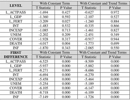
Table 1: Results of the ADF Unit Root Test

LEVEL With Constant Term With Constant and Trend Terms

T Statistic P Value T Statistic P Value

L_ACTPASS -1.694 0.427 -0.627 0.972 L_GDP -1.360 0.592 -2.107 0.527 L_FERT -3.209 0.027 -1.260 0.884 INT -1.483 0.532 -0.335 0.866 INCEXP -1.085 0.713 -1.461 0.827 UNEM -2.202 0.209 -2.451 0.349 COVER -1.928 0.317 -0.917 0.944 DEATH -4.017 0.004 -1.773 0.699 INF -1.870 0.343 -2.065 0.550 FIRST DIFFERENCE

With Constant Term With Constant and Trend Terms

T Statistic P Value T Statistic P Value

L_ACTPASS -6.525 0.000 -8.509 0.000 L_GDP -5.937 0.000 -5.882 0.000 L_FERT -8.271 0.000 -8.686 0.000 INT -6.694 0.000 -6.270 0.000 INCEXP -5.458 0.000 -5.464 0.000 UNEM -5.254 0.000 -5.189 0.001 COVER -6.105 0.000 -6.147 0.000 DEATH -8.718 0.000 -6.109 0.000 INF -7.149 0.000 -1.726 0.000

Sources: All data tables and charts presented in this study were obtained from Authors calculations. Note: The Schwarz Information Criterion (SIC) was used for the optimal lag length. L_ACTPASS, L_FERT and DEATH series were stationary, that is I(0) at level without constant and trend terms. All other series for all models were not stationary, that is I(0) at level and were stationarised after taking first differences, that is I(1).

The unit root tests are summarised in Table 1. It was mentioned that with the exception of interest rate and inflation rate, all of the variables included trend and constant terms. Upon examination of Table 1, it is found that although not all variables were stationary at level, all variables appeared stationarised after taking the first difference.

3.2. Regression Analyses

In the first stage of the analysis to be performed on sustainability of the actuarial balance, a multi-linear regression model was designed including the dependent variable active/passive ratios and the other independent variables in the data set.

(8)

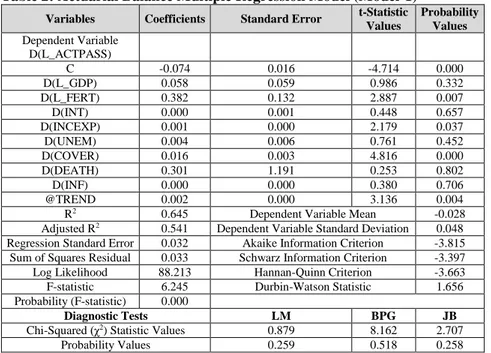
Table 2: Actuarial Balance Multiple Regression Model (Model-1)

Variables Coefficients Standard Error t-Statistic

Values Probability Values Dependent Variable D(L_ACTPASS) C -0.074 0.016 -4.714 0.000 D(L_GDP) 0.058 0.059 0.986 0.332 D(L_FERT) 0.382 0.132 2.887 0.007 D(INT) 0.000 0.001 0.448 0.657 D(INCEXP) 0.001 0.000 2.179 0.037 D(UNEM) 0.004 0.006 0.761 0.452 D(COVER) 0.016 0.003 4.816 0.000 D(DEATH) 0.301 1.191 0.253 0.802 D(INF) 0.000 0.000 0.380 0.706 @TREND 0.002 0.000 3.136 0.004

R2 _0.645 _{Dependent Variable Mean} _-0.028

Adjusted R2 _0.541 _{Dependent Variable Standard Deviation} _0.048

Regression Standard Error 0.032 Akaike Information Criterion -3.815

Sum of Squares Residual 0.033 Schwarz Information Criterion -3.397

Log Likelihood 88.213 Hannan-Quinn Criterion -3.663

F-statistic 6.245 Durbin-Watson Statistic 1.656

Probability (F-statistic) 0.000

Diagnostic Tests LM BPG JB

Chi-Squared (χ2_{) Statistic Values} _0.879 _8.162 _2.707

Probability Values 0.259 0.518 0.258

Note: Here and hereinafter D symbols, which stand infront of the variables, denote the first differences.

As seen in Table 2, Model-1 was constructed in order to measure the effects of all of the variables on actuarial balance. The regression model that was estimated is statistically significant [Prob (F-statistic) = 0.000054]. Among the diagnostic tests conducted in relation to the model were the Breusch-Godfrey LM autocorrelation test, the Breusch-Pagan-Godfrey (BPG) heteroscedasticy test, and the Jarque-Bera test of normality of residuals. The results of these tests revealed that the model did not contain autocorrelation and heteroscedasticity problems and that the residuals were normally distributed. The R2 _{value in Model-1 was found to be 0.645 Although three} independent variables fertility rate, coverage ratio were found to be significant in 1% significant level and income/expense ratio in 5% significant level in as a result of the t-tests conducted, the fact that the others were found to be insignificant even in 10% significant level is not consistent with the theoretic expectations. When this is the case, the first thing that should be considered is whether there exists a multicollinearity or not. Some of the systematic tests used to research the existence of multicollinearity include determining whether there exists a high correlation between the explanatory variables [correlations of greater than 0.8 among independent variables generally indicate multicollinearity (Allison, 1999)], comparing multiple correlations and partial correlations, and variance inflation factor (VIF) measures. A VIF>5 indicates the existence of multicollinearity (Tarı, 2018). As seen in the Correlation Matrix in Table 3, the correlation coefficients between all of the independent variables is less than 0.8. Moreover, as seen in Table 4, the VIF values of all of the independent variables are less than 5. Based on these results, it can be said that also multicollinearity problem does not exist in Model-1.

(9)

149

Table 3: Correlation Matrix

X1 X2 X3 X4 X5 X6 X7 X8 X9 X1 1.000 -0.022 -0.018 0.113 -0.158 0.116 -0.212 -0.130 -0.064 X2 -0.022 1.000 -0.055 0.040 -0.103 0.168 0.067 0.088 0.094 X3 -0.018 -0.055 1.000 -0.037 -0.207 -0.066 0.093 0.505 -0.210 X4 0.113 0.040 -0.037 1.000 -0.123 0.136 -0.144 -0.300 0.069 X5 -0.158 -0.103 -0.207 -0.123 1.000 -0.201 0.168 0.016 -0.062 X6 0.116 0.168 -0.066 0.136 -0.201 1.000 -0.113 -0.009 -0.279 X7 -0.212 0.067 0.093 -0.144 0.168 -0.113 1.000 0.209 0.208 X8 -0.130 0.088 0.505 -0.300 0.016 -0.009 0.209 1.000 -0.151 X9 -0.064 0.094 -0.210 0.069 -0.062 -0.279 0.208 -0.151 1.000

Note: X1, X2, X3, X4, X5, X6, X7, X8, and X9 represent D(L_GDP), D(L_FERT), D(INT), D(INCEXP), D(UNEM), D(COVER), D(DEATH), D(INF), and @TREND variables, respectively.

Table 4: VIF Values

X1 X2 X3 X4 X5 X6 X7 X8 X9

VIF 1.084 1.087 1.602 1.175 1.235 1.260 1.202 1.614 1.312

Note: X1, X2, X3, X4, X5, X6, X7, X8, and X9 represent D(L_GDP), D(L_FERT), D(INT), D(INCEXP), D(UNEM), D(COVER), D(DEATH), D(INF), and @TREND variables, respectively.

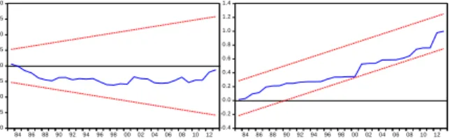
-20 -15 -10 -5 0 5 10 15 20 848688909294969800020406081012 CUSUM 5% Significance -0.4 -0.2 0.0 0.2 0.4 0.6 0.8 1.0 1.2 1.4 848688909294969800020406081012 CUSUM of Squares 5% Significance

Figure 1: CUSUM and CUSUM-SQ Charts (Model-1)

As seen in Figure 1, both the CUSUM and CUSUM-SQ charts remained between the boundaries of the 95% confidence interval. Where α stands for significance level, confidence interval is calculated as a percentage 100·(1 − α). Accordingly, 95% confidence interval correspond to 5% significance level. In order to determine whether there existed a structural break in the 1972-2013 data set included in Model-1, both a CUSUM and CUSUM-SQ structural break test were conducted. The results indicated that no structural break existed because that it is remained between the boundaries of confidence interval in both CUSUM charts.

(10)

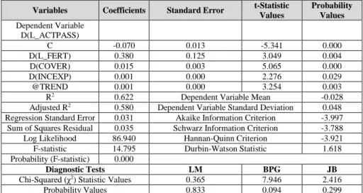
Table 6: Actuarial Balance Multiple Regression Model (Model-2)

Values Probability Values Dependent Variable D(L_ACTPASS) C -0.070 0.013 -5.341 0.000 D(L_FERT) 0.380 0.125 3.049 0.004 D(COVER) 0.015 0.003 5.065 0.000 D(INCEXP) 0.001 0.000 2.276 0.029 @TREND 0.001 0.000 3.254 0.003

Adjusted R2 _0.580 _{Dependent Variable Standard Deviation} _0.048

Log Likelihood 86.940 Hannan-Quinn Criterion -3.921

F-statistic 14.795 Durbin-Watson Statistic 1.618

Presented in Table 6, Model-2 (actuarial balance model) is also significant [Prob (F-statistic) = 0.00000]. According to the diagnostic tests related to the model, Model-2 does not contain autocorrelation or heteroscedasticity problems and the residuals are normally distributed. The R2_{value in Model-2 was found to be 0.622. In other words,} five other insignificant variables not included in Model 2 that were included in Model-1 together explained only 2.3% of the actuarial balance (64.5% - 62.2%). Lastly, it is necessary to ascertain whether any structural breaks existed in the 1972-2013 data sets included in Model-2.

Table 5: Model Selection Criteria

Model Selection Criteria Model-1 Model-2

Adjusted R2 _0.541 _0.580

Akaike Information Criterion -3.815 -3.997 Schwarz Information Criterion -3.397 -3.788

Model-2 was constructed using the general-to-specific method to remove the insignificant variables from Model-1. Compared to Model-1, Model-2 contains lower AIC and SIC values as well as a greater Adjusted R2 _{value. Model-2 is clearly seen to} be a better model than Model-1 based on both nested and non-nested model selection criteria. -20 -15 -10 -5 0 5 10 15 20 1980 1985 1990 1995 2000 2005 2010 CUSUM 5% Significance -0.4 -0.2 0.0 0.2 0.4 0.6 0.8 1.0 1.2 1.4 1980 1985 1990 1995 2000 2005 2010 CUSUM of Squares 5% Significance

Figure 2: CUSUM and CUSUM-SQ Charts (Model-2)

As seen in Model-2’s CUSUM-SQ chart (Figure 2), peaked the confidence interval in 1999 and 2000. In the CUSUM chart however, it is remained between the boundaries of the confidence interval. In such cases, although a break is observed in the

(11)

CUSUM-Sustainability of the Actuarial Balance: Turkey’s Experience Between 1972-2013

151

SQ chart, since such a break is not encountered in the CUSUM chart, it is disregarded (Brown, Durbin and Evans, 1975: 159; Tarı and Bozkurt, 2006: 20).

3.3. Johansen Cointegration Analysis

In the previous section, Model-2 (actuarial balance model) was constructed by removing those variables found to be insignificant in Model-1. Since Model-2 was then determined to be a better model according to both nested and non-nested tests, Model-2 will be used in all analyses henceforth.

Table 7: Selection Criteria in Determining Lag Length

Note: LR: Likelihood Ratio, FPE: Final Prediction Error, AIC: Akaike Information Criterion, SIC: Schwarz Information Criterion, HQ: Hannan-Quinn Information Criterion. * indicates the lag length chosen by the related criteria.

As is the case in single response variable models, the optimal value of lag length p value is also unknown in practice in VAR models. The selection criteria in determining lag length can be found in Table 7. According to LR, FPE, and AIC criteria, the optimal lag length, in other words the lowest value was three whereas according to SIC and HQ criteria, it was 1. Since the three information criteria recommended, lag length was selected as 3. (Sevüktekin and Çınar, 2014).

Table 8: Johansen Cointegration Test Results Null Hypothesis Alternative Hypothesis Trace Statistic 5% critical value 1% critical value Null Hypothesis Alternative Hypothesis Maximum Eigenvalue Statistic 5% critical value 1% critical value r = 0 r>0 **92.407 53.120 60.160 r = 0 r=1 **50.055 28.140 33.240 r ≤ 1 r>1 **42.352 34.910 41.070 r ≤ 1 r=2 20.519 22.000 26.810 r ≤ 2 r>2 *21.832 19.960 24.600 r ≤ 2 r=3 *17.915 15.670 20.200 r ≤ 3 r>3 3.917 9.240 12.970 r ≤ 3 r=4 3.917 9.240 12.970

Note: The cointegration test was performed by using the cointegrating equation with a constant term and no trend term and the VAR model with no constant and trend terms. A lag length of 2 was used. r indicates the number of cointegrating vectors. Critical values were taken from Osterwald-Lenum (1992: 467). *, and ** indicates that the null hypothesis was rejected at significance level of 5% and 1%, respectively.

-.1 .0 .1 .2 .3 .4 .5 1975 1980 1985 1990 1995 2000 2005 2010 Cointegrating relation 1 .00 .05 .10 .15 .20 .25 .30 1975 1980 1985 1990 1995 2000 2005 2010 Cointegrating relation 2

Figure 3: Cointegrating Relation Charts

When the results of Johansen’s Cointegration Test presented in Table 8 are examined, at the 1% significance level while the trace statistic implied the existence of two cointegrating vectors, the maximum eigenvalue implied that there was a single cointegrating vector. In the case that the trace statistic and the maximum eigenvalue statistic imply a different number of cointegrating vectors, Johansen and Juselius’ (1992: 220-223) method is followed in order to determine the number of cointegrating vectors to be taken into consideration. Johansen and Juselius named r≤ (m-1) as

Lag LR FPE AIC SIC HQ

0 NA 0.0114 6.8774 7.2187 6.9998

1 182.0365 0.0001 2.1817 *3.2053 *2.5489

2 *21.8955 0.0001 2.2472 3.9534 2.8593

(12)

reduced rank whereas m indicates the number of variables. If the trace statistic and maximum eigenvalue statistics show a different number of cointegrating vectors in the reduced rank, then stationary of the cointegrating charts are observed. If the cointegrating relationship charts of the ranks implying a higher number appear to be stationary, the rank implying a higher number is accepted. Otherwise, the rank implying a lower number is accepted. In addition to this, Lütkepohl, Saikonnen and Trenkler (2001: 15) stated that although the two tests are of equal power, trace statistic tests are more effective than maximum eigenvalue tests for short-run samples. When the cointegrating relation charts included in Figure 3 are examined according to Johansen and Juselius’ method, it is clearly observed that 1 cointegrating vector should be accepted, just like the maximum eigenvalue statistic had indicated. A single cointegrating vector was accepted and the analysis continued. The normalised vector is presented in Table 9. Upon examination of the normalised cointegrating vector in Table 9, fertility rate, from among all variables, were observed to have the greatest effect on active/passive ratios. Using normalised coefficients, the equation showing the long-run relationship is shown below:

   

_ 5.4753 3.074 _ 0.0427 0.0095

L ACTPASS  L FERT  COVER  INCEXP (5)

Table 9: Normalised Cointegrating Vector

L_ACTPASS (-1) L_FERT (-1) COVER (-1) INCEXP (-1) C

Coefficient 1 3.074028 0.042761 -0.009566 -5.475322

Standard Error -0.7109 -0.01076 -0.00189 -1.33184

t-Statistic Value [ 4.32415] [ 3.97354] [-5.06033] [-4.11110]

Probability Value 0.00010 0.00030 0.00001 0.00020

Note: t-statistic values were converted to probability values by using the following link.: http://www.danielsoper.com/statcalc3/calc.aspx?id=8 (16.07.2015). Two-tailed t-test was used. All coefficients are significant at the 1% significance level.

Fertility rate, SGK’s coverage ratio, and income/expense ratio are observed to be effective on the long-run actuarial balance (active/passive ratios) ambiguity in Turkey. In order to determine whether possible deviations in the long-run relationship would be corrected in the short-run, an error correction model (ECM) should be constructed.

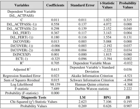
3.4. Error Correction Model (ECM)

In Table 10, the results of the error correction model are presented. It is observed that the adjustment coefficient of the error correction term included in the model is -0.325. As expected, the adjustment coefficient was between -1 and 0. Since this result confirmed the long-run relationship in the actuarial balance model, it can be said that the balancing mechanism, by decreasing deviations from the long-run balance by approximately 33% each year, is effective in bringing the model into balance.

(13)

153

Table 10: Error Correction Model Results

Values Probability Values Dependent Variable D(L_ACTPASS) C 0.011 0.011 1.023 0.315 D(L_ACTPASS(-1)) 0.558 0.137 4.072 0.000 D(L_ACTPASS(-2)) 0.298 0.139 2.152 0.040 D(L_FERT) 0.367 0.117 3.143 0.004 D(L_FERT(-1)) 0.180 0.116 1.554 0.131 D(COVER) 0.013 0.003 5.088 0.000 D(COVER(-1)) -0.006 0.003 -2.192 0.037 D(COVER(-2)) -0.008 0.004 -2.222 0.034 D(INCEXP) 0.001 0.000 1.815 0.080 ECT(-1) -0.325 0.096 -3.394 0.002

Adjusted R2 _0.613 Dependent Variable’s Standard

Deviation 0.036

Log Likelihood 98.159 Hannan-Quinn criterion -4.368

F-statistic 7.689 Durbin-Watson statistic 2.222

3.5. VAR/VEC Models

The traditional economic approach used until the 1970s was abandoned for a number of reasons following the 1970s. In his radical critique, as was stated in Lucas’ own critique, Sims (1980) criticised the fact that during the preparation stage of the policy making process, macro-economic policy makers very frequently used simultaneous models that act arbitrarily not only when making distinction between endogenous and exogenous variables, but also when limiting parameters. Instead, Sims advocated VAR models, in which all variables were included as endogenous variables in the system. In addition to together being called innovation accounting, the impulse-response and variance decomposition analyses used in VAR/VEC models are considered to be extremely useful tools for observing relationships among economic variables (Enders, 2004).

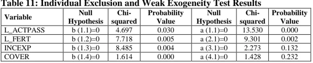
3.5.1. Individual Exclusion and Weak Exogeneity Tests

Individual exclusion and weak exogeneity hypotheses are expressed as H0:b 11=0, H0:b 12=0, H0:b 13=0, H0:b 14=0 and H0: a 11=0, H0: a 21=0, H0: a 31=0, H0: a 41=0, respectively. Weakly exogenous variables appear solely on the right-hand side of the equation whereas endogenous variables appear on the left-hand side of the equation (Metin and Üçdoğruk 1998: 283). Since weakly exogenous variables are excluded from the vector on the left-hand side of the equation, their short-run behaviours are not modelled, they yet remain in the long-run model. If weakly exogenous variables are also found to be insignificant in the long-run cointegration space according to the individual exclusion test, they can be excluded from the system (Harris and Sollis, 2003). At the 5% significance level, while all variables were found to be significant in the long-run cointegration space according to the results of the individual exclusion test, both income/expense ratio and coverage ratio was found to be weakly exogenous

(14)

according to the results of the weak exogeneity test. According to the same weak exogeneity test neither active/passive ratio nor fertility rate was found to be weakly exogenous. No weakly exogenous variables were excluded from the system.

Table 11: Individual Exclusion and Weak Exogeneity Test Results

Variable Null Hypothesis Chi-squared Probability Value Null Hypothesis Chi-squared Probability Value L_ACTPASS b (1.1)=0 4.697 0.030 a (1.1)=0 13.530 0.000 L_FERT b (1.2)=0 7.718 0.005 a (2.1)=0 9.301 0.002 INCEXP b (1.3)=0 8.485 0.004 a (3.1)=0 2.273 0.132 COVER b (1.4)=0 1.614 0.000 a (4.1)=0 1.428 0.232 3.5.2. Impulse-Response Analysis

1. In order to perform a correct impulse-response analysis, variables must be clockwise ordered as from the most exogenous to the most endogenous. While ordering variables in such a way, either prior knowledge acquired from economic theory or causality relationships obtained using the Granger causality test are benefited from (Enders, 2004). Using results from the Granger Causality table included in Appendix 1 (Bozdağlıoğlu and Özpınar, 2011: 52), an order of L_ACTPASS, L_FERT, INCEXP and COVER (from the highest number of granger-causes to the lowest number of granger-granger-causes) was deemed appropriate. Appendix 2 presents the Impulse-Response Analysis Charts.

3.5.3. Variance Decomposition

A variance decomposition analysis shows the ratio between variances resulting from a variable’s own shocks and the variances resulting from other variables’ shocks. In other words, the variances appearing in one variable show the degree of interpretation of the other variables used in the model (Sevüktekin and Çınar, 2014). Variance decomposition tables are presented in Appendix 3. The important thing here is that 31% of variances in social security institutions’ income/expense ratios during the first period and roughly 50% of variances from the final period stem from the same institutions’ active/passive ratios. Such a powerful explanatory relation that active/passive ratio had over the income/expense ratios, proved that active/passive ratios, the most commonly used criteria in measuring financial balances of social security institutions in Turkey, were a good indicator.

3.5.4. Future Predictions for the Variables

VAR/VEC models are used extensively in making predictions concerning time series. In this context, VAR/VEC models are accepted as being among the most effective prediction methods in the literature. While making macro-economic predictions, it is observed that not only VAR/VEC models composed of three or four variables are more commonly used, but also the inclusion of a higher number of endogenous variables may lead to inconsistent predictions, due to mutlicollinearity (Başar, 2007: 19, 20). The prediction charts, which span until 2050, of the variables used in the VEC model predicted in the present study are presented in Appendix 4. While examining the prediction charts of the variables, the 2013 active/passive ratio of 1.9 and fertility rate of 2.09 were predicted to reach 1.72 and 2.33, respectively, in 2050. The 2013 SGK coverage ratio of 81.9% and income/expense ratio of 89.23% were both predicted to be approximately 73% in 2050.

(15)

155

4. Conclusion and Evaluations

Based on three different models for the 1972-2013 period, findings related to the sustainability of Turkey’s actuarial balance are presented as follows:

i) The coverage ratio found to increase the pension system’s active/passive ratio in the short-run was found to decrease the same ratio in question in the long-run. In the light of these findings:



It is evident that fundamental principle of an insurance system presuming every single worker and every individual with a job be compulsorily insured is not viable in Turkey and due to economic reasons, when the number of dependents without their own insurance is compared to the number of actively insured individuals paying insurance premiums, it is observed that the system is running beyond viable capacity. In this respect, in order for the actuarial balance to be affected positively in the long-run, it is necessary to expand social security coverage to the number of individuals paying a premium instead of to dependents.

ii) Fertility rate found to increase the pension system’s active/passive ratio in the short-run was found to decrease the same ratio in question in the long-short-run. In the light of these findings:



An increase in the active/passive ratio is linked to an increase in the ratio between actively insured individuals and number of retired individuals and/or dependents receiving insurance benefits in the system. Although the Pension Reform initiated by law number 4447 began to gradually increase the age of retirement, the expected decrease in numbers of passively insured individuals has not been realised. While this process continues, it does not seem possible to increase the age of retirement again. For this reason, whether an increase in fertility rate has a positive effect on the actuarial balance in the long-run is bound to whether young individuals are included in the pension system as actively insured individuals or not.



An increase in the youth population’s education, carrier, and employment opportunities is necessary. In this respect, not only do the necessary incentives need to be provided directly by the government or by means of social security institutions, so do the necessary precautions need to be taken. iii) The pension system’s income/expense ratio was found to increase the active/passive ratio in both short- and long-run. Moreover, active/passive ratios, the most commonly used criteria in measuring financial balances of social security institutions in Turkey, were proven to be a good indicator. In the light of these findings:



First, social security institutions’ expenditures should be disciplined and transfers from the general budget to social security should be reduced. In order to achieve this, previously applied programmes, such as early retirement, debt service, and premium amnesty should not be reinstated. Foreign debt service, however, should be reviewed from a benefit-cost perspective.



In order to increase social security institutions’ income, it is recommended that informal employment be reduced, controls be increased, and formal employment be encouraged.



Premium collection related problems need to be solved and pension funds should be used in productive areas.

(16)

For Turkey, it is predicted that the active/passive ratios will fall below the signal level. In conclusion, the actuarial balance during 1973-2013 was proved to be not sustainable.

5. References

Acar, İ. A. and Kitapcı, İ. (2008). Sosyal güvenliğin demografik boyutu: Türkiye’deki emeklilik sistemindeki değişim. Maliye Dergisi, (154), 77-98.

Akyıldız, H. and Yavuz, A. (2007). Türkiye’de sosyal güvenliğin finansman açıklarının temel dinamikleri üzerine bir analiz. Karamanoğlu Mehmetbey Üniversitesi İktisadi ve İdari Bilimler Fakültesi Dergisi, 2(3), 424-437.

Allison, P. D. (1999). Multiple regressions: A primer. California: Thousand Oaks Pine Forge Press.

Alparslan, A. (2005). A genetic algorithm-based search for parametric reform alternatives for the Turkish pension system: 2005-2060 (Unpublished master thesis). Bilkent Üniversitesi Sosyal Bilimler Enstitüsü İktisat Anabilim Dalı, Ankara.

Başar, S. (2007). Türkiye için bir makro iktisadi öngörü modeli. İktisat, İşletme ve Finans Dergisi, 22(254), 18-27.

Boado-Penas, M. del and Vidal-Meliá, C. (2013). The actuarial balance of the pay-as-you-go pension system: The Swedish NDC model versus the US DB model. Holzmann, R., Palmer, E. and Robalino, D. (Ed.) Non-financial Defined Contribution (NDC) Pension Systems: Progress and New Frontiers in a Changing Pension World içinde (443-479 ss.) The World Bank, Washington. Boado-Penas, M. del, Sakamato, J. and Vidal-Meliá, C. (2009). Models of the

actuarial balance of the pay-as-you-go pension system. A review and some lessons. 4th International colloquium of the IAA pension, benefits and social security section içinde (1-19. ss.)

Bozdağlıoğlu, E. Y. ve Özpınar, Ö. (2011). Türkiye’ye gelen doğrudan yabancı yatırımların Türkiye’nin ihracat performansına etkilerinin VAR yöntemi ile tahmini. Dokuz Eylül Üniversitesi Sosyal Bilimler Enstitüsü Dergisi, 13(3), 39-63.

Brown, R. L, Durbin, J. and Evans, J. M. (1975). Techniques for testing the constancy of regression relationships over time. Journal of the Royal Statistical Society, 37(2), 149-192.

Bulutay, T. (1995). Employment, unemployment and wages in Turkey. Ankara: ILO Publications.

Congress of the United States (2013). The 2013 long-term projections for social security: additional information. John, S. (Ed.) Erişim adresi

https://www.cbo.gov/sites/default/files/113th-congress-2013-2014/reports/44972-SocialSecurity.pdf

Enders, W. (2004). Applied econometric time series. (2th ed.). New York: John Wiley Publications.

Engle, R. F. and Granger, C.W.F. (1987). Co-integration and error correction: Representation, estimation, and testing. Econometrica, 55(2), 251-276. Granger, C.W.J. and Newbold, P. (1974). Spurious regressions in econometrics.

Journal of Econometrics, 2(2), 112-120.

Güner, T. (2012). Türkiye’de primli sosyal güvenlik sisteminin finansman yapısının analizi. (Unpublished master thesis). Isparta Üniversitesi Sosyal Bilimler Enstitüsü Çalışma Ekonomisi ve Endüstri İlişkileri Anabilim Dalı, Isparta.

(17)

157

Harris, R. and Sollis, R. (2003). Applied time series modelling and forecasting. (1st ed.). Chicester: John Wiley Publications.

Hendry, D. F. and Ericsson, N. R. (1991). An econometric analysis of U.K. money demand in monetary trends in the United States and the United Kingdom by Friedman, M. and Schwartz, A.J. American Economic Review, (81), 8-38. Johansen, S. and Juselius, K. (1990). Maximum likelihood estimation and inference

on cointegration-with applications to demand for money. Oxford Bulletin of Economics and Statistics, (52), 69-210.

Johansen, S. and Juselius, K. (1992). Testing structural hypotheses in a multivariate cointegration analysis of the PPP and the UIP for UK. Journal of Econometrics, (53), 211-244.

Keskin, M. (2006). Türkiye’de sosyal güvenlik açığı bir doğrusal optimizasyon analizi. (Unpublished master thesis) Marmara Üniversitesi Sosyal Bilimler Enstitüsü İşletme Anabilim Dalı, İstanbul.

Lee, R. and Tuljapurkar, S. (1998). Stochastic forecasts for social security. Wise, D. (Ed.) Frontiers in the economics of aging içinde (393-428. ss.) University of Chicago Press, Chicago.

Lee, R., Anderson, M.W. and Tuljapurkar, S. (2003). stochastic forecasts of the social security trust fund. University of Michigan Retirement Research Center, (043), 1-36.

Lütkepohl, H., Saikkonen, P. and Trenkler, C. (2001). Maximum eigenvalue versus trace tests for the cointegrating rank of a VAR Process. Econometrics Journal, 4(2), 1-29.

Mattil, B. (2006). Pension systems: Sustainability and distributional effects in Germany and United Kingdom. Germany: Physica-Verlag.

Metin, K. and Üçdoğruk, Ş. (1998). Türk imalat sanayinde uzun dönem ücret-fiyat-istihdam ilişkilerinin ekonometrik olarak incelenmesi. Çukurova Üniversitesi İktisadi ve İdari Bilimler Fakültesi Dergisi, 8(1), 279-287.

Osterwald-Lenum, M. (1992). A note with quantiles of the asymptotic distribution of the ML cointegration rank test statistics. Oxford Bulletin of Economics and Statistics, 54, 461-472.

Plamondon, P., Drouin, A., Binet, G., Cichon, M., Mcgillivray, W.R., Bédard, M. and Perez Montas, H. (2002). Quantitative methods in social protection series: Actuarial practice in social security. Geneva: Oxford-ILO Publications.

Roach, B. and Ackerman, F. (2005). Securing social security: Sensitivity to economic assumptions and analysis of policy options. GDAE Working Paper, 05(03), 1-32. Sayan, S. (2005). Sosyal sigortalar kurumu’nun uzun dönem aktüeryel dengeleri: 1999 reformu ve alternatifleri. Muğla Üniversitesi İktisadi ve İdari Bilimler Fakültesi Dergisi, (1), 29-55.

Sevüktekin, M. and Çınar, M. (2014). Ekonometrik zaman serileri analizi. (4.bs.) Bursa: Ezgi Matbaacılık.

SGK (2015). Erişim adresi www.sgk.gov.tr

Sims, C. A. (1980). Macroeconomics and reality. Econometrica, 48(1), 1-48. Tarı, R. ve Bozkurt, H. (2006). Türkiye’de istikrarsız büyümenin var modelleri ile

analizi (1991.1-2004.3), İstanbul Üniversitesi Ekonometri ve İstatistik Dergisi, (4): 12-28.

Tarı, R. ve Yıldırım, D. Ç. (2006). Döviz kuru belirsizliğinin ihracata etkisi: Türkiye için bir uygulama, Yönetim ve Ekonomi Dergisi, 16(2), 95-105.

(18)

Tuna, G. (2009). Genel sağlık sigortası primini basamaklandırmanın aktüeryal denge üzerine etkisi. (Sosyal güvenlik kurumu uzmanlık tezi). Sosyal Güvenlik Kurumu, Ankara.

Ündemir, Y. G. (2009). Sosyal güvenliğin önemli değişkenlerinin zaman serileri analizi ile öngörüsü. (Sosyal güvenlik kurumu uzmanlık tezi). Sosyal Güvenlik Kurumu, Ankara.

Yaşarlar, Y. (2016). Aktüeryal dengenin sürdürülebilirliği: Türkiye deneyimi. (Unpublished PhD. thesis). İstanbul Üniversitesi Sosyal Bilimler Enstitüsü İktisat Anabilim Dalı, İstanbul.

Yerdelen Tatoğlu, F. (2018). İleri panel veri analizi-Stata uygulamalı. (3.bs.). İstanbul: Beta Yayıncılık.