1. Introduction
As a matter of fact, growth of the Turkish economy has been remarkable during the last decade, while it also has been relatively stable as compared to the previous decades and to the economies of developing and developed countries in general. Accordingly, there has also been significant increase in foreign trade. The volume of Turkey’s foreign trade during the period under concern (1989-2012) has increased from to US Dollar 27.4 billion to US Dollar 375.6 billion. However, the increase during the last decade is even more remarkable from US Dollar 72.7 billion to US Dollar 375.6 billion that is more than 416%. However, the crucial point may not be this increase but the change in the structure of the foreign trade and the trade deficit. That is this increase has not been distributed uniformly among Turkey’s top trading partners on one hand, and on the other, while volume of trade increased at the same time the current account deficit increased, and even relatively faster. According to data from the World Bank Development Indicators, the current account deficit as the percentage of GDP is 9.94% in 2011 and is the highest among G20 economies. So, one should take more seriously the rate of increase in imports rather than the increase in total volume of trade.
This paper aims to estimate import demand functions in Turkey. However, different from many studies, we focus on the disaggregated import demand functions, namely for capital goods, intermediate inputs and consumption goods imports, instead of aggregated import demand. We point out the differences in short-run elasticity and long-run elasticity for three different categories of imports. Therefore, our empirical findings can be noteworthy for both the Turkish economy and its main trading partner economies, such as the European Union, the Russian Federation, China PR and the United States (Gozgor 2011). Particularly, it can be important to know the effects of exchange rate changes on specific categories of imports in Turkey thereby one can see how possible deprecation in the real value of the Turkish Lira affects different groups of imports and in terms of current account balance deficit. Furthermore, decomposition of total imports is important in Turkey because import demand for some goods is critical not only to reduce current account deficit, but also to provide sustainable economic growth and export promotion. In this case, intermediate goods imports are particularly important because almost 70% share of total imports is intermediate inputs in the Turkish economy over related period (Ketenci and Uz 2010).
Aggregated import dynamics in Turkey have intensively examined in the literature, such as that by Kotan and Saygili (1999), Aydin et al. (2004), Bahmani-Oskooee and Kara (2005) and Yavuz and Guris (2006). Only two studies had attempted to investigate the disaggregated import demand in Turkey (Togan and Berument 2007; Aldan et al. 2012).1 Togan and Berument (2007) used cointegration technique of Johansen in order to estimate long-run price elasticity and income elasticity of disaggregated imports, namely consumption goods, capital goods and non-energy intermediate goods imports. They used the annual data for the period from 1970 to 2005. They found that long-run coefficients of domestic demand and real exchange rate were greater in consumption goods imports, as compared to capital goods and non-energy intermediate goods import demand. In addition, the long-run elasticity of domestic demand was higher than real exchange rate in all cases. Aldan et al. (2012) investigated the short-run dynamics of (disaggregated) import demand in Turkey, namely consumption goods, capital goods except transportations vehicles, transportation vehicles incidental to industry, and non-energy intermediate goods imports, for the period from 2003 to 2011 in the quarterly data set. They used the Kalman filter to obtain time-varying parameters in the ordinary least square (OLS) state-space framework and found that income
1
Limited number of studies in literature investigated the disaggregated import demand in other developing or developed economies. For instance, see Senhadji (1998), Pattichis (1999), Mah (2000) and Fukumoto (2012).
elasticity of import demand was higher than real exchange rate, except for capital goods excluding transportation. They also realized a significant heterogeneity in response of imports to GDP and real exchange rate both through different sectors and through time; particularly in period of the great global recession although their methodology did not give opportunity to investigate the period of great global recession and to use time trend. Perhaps, they also realized that a further study would contribute to their empirical findings. Finally, they concluded in the favor of “aggregation bias”, where there was a significant difference between direct and indirect estimations (Khan 1975).
This study attempts to make two contributions to the existing literature. First, we systemically focus on the disaggregated import demand functions instead of aggregated demand of the Turkish imports, unlike the other studies. To the best of our knowledge, this paper is the first to estimate the short-run and at the same time long-run disaggregated import functions for Turkey. Secondly, related to our aim, the methodology used and the period covered, which also include impacts of the great global recession differ from other studies.
The remainder of this paper is organized as follows. Next section explains the methodology, the model specifications and the data. Third section discusses the empirical findings, and final section is the concluding remarks.
2. Methodology, Model Specifications and Data
This paper investigates both the short-run and the long-run dynamics of disaggregated import demand in Turkey and in terms of the period over the ‘global trade collapse’.2 Just as in the case of Bahmani-Oskooee and Kara (2005) and Yavuz and Guris (2006), we use Autoregressive Distributed Lag (ARDL) model because this model allows estimating both short-run and long-run coefficients. On the other hand, ARDL model has an advantage compared to other cointegration techniques because it is free from the assumption of same integration degree of as I(1) in cointegrating series (Pesaran et al. 2001). We re-examine long-run estimations by using Dynamic Ordinary Least Squares (DOLS) technique, and also aim to control the effects of seasonality, time trend, the periods of the floating exchange rate regime and the great global recession. Doing so, in a way we check the econometric robustness of main empirical findings of the ARDL model.
Actually, there are a number of efficient methods for estimating the cointegrating relationship in literature.3 In this paper, we use DOLS technique, just because it outperforms similar approaches, such as error correction models, particularly in small samples.4 Given the relatively small sample in this study, we ignore maximum likelihood multivariate approach of Johansen (1988, 1991) and Johansen and Juselius (1990). Thus, we somewhat follow a similar methodology which is also used by Cheung et al. (2012).
The effects of income and the real exchange rate on import demand are well-known in literature. Imports demand, exports demand, and the movements of trade balance are explained by changes in relative prices, exchange rate and income in the imperfect substitute model of Goldstein and Khan (1985). For the disaggregated import demand function, we
2 The period of recent global recession also called as ‘the global trade collapse’ in literature. We believe that investigating the impact of global recession on import demand is also important because the global recession and financial turmoil from 2008 to 2009 was related with a dramatic collapse in world international trade, in excess of the fall in production, and this significantly larger than the fall in GDP (Gopinath et al. 2012).
3 For instance, Phillips and Hansen (1990) proposed an estimator called the Fully Modified Ordinary Least Square (FMOLS). This method is asymptotically unbiased and has fully efficient mixture normal asymptotics permits standard Wald tests by using asymptotic Chi-square statistical inference. Similarly, Park (1992)’s Canonical Cointegrating Regression (CCR) estimator follows a mixture normal distribution which is free of non-scalar nuisance parameters, and allowing for asymptotic Chi-square testing procedure.
follow this theoretical framework, and assume that foreign and domestic products are imperfect substitutes, such as
*
( / , )
it xit t t
X f P P Y (1) In this function, X is it type of disaggregated import value in Turkey, it *
/
xit t
P P is the real effective exchange rate in Turkey and Y is the Real Gross Domestic Product (GDP) in the t
Turkish Lira (TRY). Following this simple model, we basically estimate six equations those in the logarithmic form of disaggregated imports demand functions in Turkey as follows:
0 1 2 3 1
lnCAGt lnGDPt lnREERtCONTROLt (2a)
4 5 6 7 2
lnCAGt lnGFCFt lnREERt CONTROLt (2b)
0 1 2 3 3
lnIGt lnGDPt lnREERt CONTROLt (3a)
4 5 6 7 4
lnIGt lnEXt lnREERt CONTROLt (3b)
0 1 2 3 5
lnCOGt lnGDPt lnREERtCONTROLt (4a)
4 5 6 7 6
lnCOGt lnDCt lnREERt CONTROLt (4b)
- Where, LNCAG= Natural logarithm of Capital Goods Imports (in the USD). Data
Source: The Turkish Statistical Institute (TSI).
- LNGDP= Natural logarithm of Real Gross Domestic Product (GDP) (in the Turkish
Lira (TRY) and GDP Deflator is used 2003=100). Data Source: The International Monetary Fund (IMF).
- LNREER= Natural logarithm of the Real Effective Exchange Rate Index: (the
consumer price index (CPI) based is used 2003=100). Data Source: The Central Bank of the Republic of Turkey (CBRT).
- LNGFCF= Natural logarithm of Real Gross Fixed Capital Formation (in the TRY,
GDP Deflator is used 2003=100). Data Source: IMF.
- LNING= Natural logarithm of Intermediate Goods Imports (in the USD). Source: TSI. - LNEX= Natural logarithm of Goods and Services Exports (in the USD). Data Source:
TSI.
- LNCOG= Natural logarithm of Consumption Goods Imports (in the USD). Data
Source: TSI.
- LNDC= Natural logarithm of Real Domestic Credit in Banking Sector (not includes
bank-to-bank loans) (in the TRY, the CPI is used 2003=100). Data Source: CBRT.
- Control variables (CONTROL) are FLO= Exchange Rate Regime Shift Dummy
Variable (Floating Exchange Rate=1, t≥2001Q2). REC= the Great Recession Dummy Variable (REC09=1 (t=09Q1, 09Q2, 09Q3)). Q1, Q2, Q3: The Quarter Dummy Variables. Trend: The Time Trend Variable.
This paper estimates disaggregated import demand functions for three different categories of imports of Turkey, for the period from 1989Q1 to 2012Q1 in the quarterly data set. In our estimations, the main determinants of disaggregated imports are GDP and REER, where their coefficients indicate the income elasticity and price elasticity, respectively.5 Each equation in above includes the control variables as “constant term”, “time trend term”, “FLO”, “REC09”, “Q1, Q2 and Q3” in DOLS estimations. We consider a proxy variable for each disaggregated
5
Yin and Hamori (2011) and Wang and Lee (2012) recently followed similar model and methodology but they estimated the aggregated import demand functions for China PR.
imports demand estimation. We use GFCF as a proxy variable of GDP in our first estimation of capital goods imports. We investigate the effect of GFCF on capital goods imports since it can be accepted as the main component and indicator of capital formation in Turkey. On the other hand, we consider exports as a proxy variable for intermediate goods imports, because the main motivation of intermediate goods imports is to produce tradable goods in Turkey. In this context, we also use domestic credits as a proxy variable in the estimations of consumption goods imports. One can suggest that disposable income may also be used instead of domestic credits in the estimation of consumption goods imports function; however, quarterly disposable income data are not available over the related period for Turkey. Thus, following Cheung et al. (2012), we suggest that domestic credits also be an indicator of the domestic demand in Turkey, particularly when recent developments in the Turkish economy are considered.6
By using these proxy variables, we aim to check not only the econometric robustness of our findings, but also the theoretical robustness of related estimations. Theoretical framework of import demand also indicates that import demand directly effects the value of aggregate GDP, because (GDP= C+I+G+X-M) where C is the consumption, I is the investment, G is the government expenditure, X is the aggregate exports and M is the aggregate imports. Therefore, we also estimate the income elasticity of import demand by using other kind of domestic income and domestic demand indicators instead of GDP.
On the other hand, Togan and Berument (2007) and Aldan et al. (2012) both in their studies used the Broad Economic Classification (BEC) of the related TSI data as we did. Although the three studies based the disaggregation and specifications of variables on the BEC, the specifications differ slightly from each other. Namely, Togan and Berument (2007) and Aldan et al. (2012) used non-energy intermediate input imports data whereas in this study we use total intermediate input imports of Turkey. As a matter of fact, in BEC classification, there is no specific-term standing for energy import demand. There is an unknown import item so called ‘confidential data’ under the heading of intermediate inputs imports.7 Therefore, we don’t consider ‘confidential data’ as energy imports demand, and used the total intermediate input imports of Turkey.
3. Empirical Findings
In this section, we firstly examine stochastic properties of variables, and report the results from unit root test of Phillips and Perron (1988) and Zivot and Andrews (1992) in Table I. As one can be seen in Table I, results from the Phillips and Perron (PP) and the Zivot and Andrews (ZA) unit root test show that the integration degrees of series are different. However, results from the ZA unit root test show that dependent variables of each regression (lnCAG, lnING and lnCOG) are stationary. Therefore, we use ARDL model.
We report the results of ARDL model in Table II and Table III. We also check the robustness of results from ARDL model by using DOLS, and report the findings in Table IV. Empirical findings basically suggest that there are significant short-run and long-run relationships between the estimated coefficient of price elasticity and income elasticity and disaggregated imports demands. In ARDL models, assumptions of no serial correlation in error terms, normally-disturbed and homoskedastic error terms are successfully satisfied. Also, results of the Ramsey-Reset test do not reject null hypothesis of the correct model specifications. We find that coefficients of the error correction mechanism in ARDL models are also significant.
6 We refer the recent and ongoing increasing real domestic credits demand in Turkey, and effects of monetary policy framework on real domestic credits demand.
Table I. Results of the Phillips-Perron (PP) and Zivot-Andrews (ZA) unit root tests Constant PP CV 1% CV 5% ZA CV 1% CV 5% Break LnCAG -1.62 -3.50 -2.89 -5.10 -5.34 -4.93 2000Q4 LnING -0.76 -3.50 -2.89 -4.95 -5.34 -4.93 2004Q1 LnCOG -1.92 -3.50 -2.89 -5.84 -5.34 -4.93 2000Q4 lnGDPt -3.09 -3.50 -2.89 -4.11 -5.34 -4.93 1999Q1 LnREERt -1.88 -3.50 -2.89 -5.42 -5.34 -4.93 1994Q1 lnGCFCt -2.44 -3.50 -2.89 -4.66 -5.34 -4.93 1998Q4 LnEX -0.04 -3.50 -2.89 -3.79 -5.34 -4.93 2003Q4 LnD 0.69 -3.50 -2.89 -2.87 -5.34 -4.93 2005Q2 Constant+Trend PP CV 1% CV 5% ZA CV 1% CV 5% Break LnCAG -4.56 -4.06 -3.45 -5.18 -5.57 -5.08 2000Q4 LnING -2.97 -4.06 -3.45 -5.66 -5.57 -5.08 2004Q1 LnCOG -3.91 -4.06 -3.45 -5.85 -5.57 -5.08 2000Q4 LnGDPt -8.59 -4.06 -3.45 -4.18 -5.57 -5.08 2000Q4 LnREERt -3.55 -4.06 -3.45 -5.41 -5.57 -5.08 1994Q1 lnGCFCt -3.73 -4.06 -3.45 -5.03 -5.57 -5.08 2000Q4 LnEX -3.43 -4.06 -3.45 -3.58 -5.57 -5.08 2003Q4 LnDC -1.21 -4.06 -3.45 -5.12 -5.57 -5.08 2001Q2
Notes: CV: Critical Value. Phillips and Perron (PP) (1988) unit root test is defined by using Barlett Kernel and
bandwidth selection method of Andrews (1991). Series have a unit root according to the null hypothesis of the PP unit root test. Series have a unit root with a structural break in constant and trend terms according to the null hypothesis of the Zivot-Andrews (ZA) unit root test.
Table II. Results of the bounds tests for cointegration analysis
Bounds Test Results F-statistic 95% Lower Bound 95% Upper Bound LM-statistic 95% Lower Bound 95% Upper Bound Capital Goods I 6.888 3.877 4.971 20.66 11.63 14.91 Capital Goods II 3.937 3.877 4.971 11.81 11.63 14.91 Intermediate Goods I 4.211 3.877 4.971 13.63 11.63 14.91 Intermediate Goods II 6.451 3.877 4.971 17.62 11.63 14.91 Consumption Goods I 6.744 3.877 4.971 18.23 11.63 14.91 Consumption Goods II 4.129 3.877 4.971 12.75 11.63 14.91
Notes: If the calculated F-statistics and LM-statistics are smaller than the lower bound that means null
hypothesis of no cointegration cannot be rejected. Critical values are given in Pesaran et al. (2001).
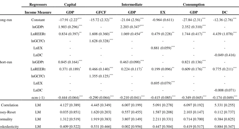
As can be seen in Table III, the coefficients of GDP and REER are statistically significant both in short-run and long-run estimated by ARDL model for all disaggregated imports demand. However, as a proxy variable instead of GDP, while GFCF and EX are also significant, DC is not significant both in the short-run and long run. Our results from ARDL model also show that coefficients of GPD are greater than coefficient of REER both in the short-run and the long-run. This main result is also confirmed in the long-run findings from DOLS estimation in Table IV. Results from ARDL model suggested if GDP increases at 1%, import demand will rise 1.90%, 2.20% , 2.35% in the long-run; and 0.84%, 0.46%, 0.82% in the short-run for capital, intermediate, and consumption goods imports, respectively. If REER rises at 1%, import demand would increase 0.83%, 1.06%, 1.74% in the long-run; and 0.37%, 0.22%, 0.61% in the short-run for capital, intermediate, and consumption goods imports, respectively. These coefficients are significant, and slightly be changed in the second frameworks of disaggregated import demands in Column II, Column IV and Column VI.
Table III. The estimated long-run and short-run coefficients by ARDL model
Regressors Capital Intermediate Consumption
Income Measure GDP GFCF GDP EX GDP DC Long-run Constant -17.91 (2.22)*** -15.72 (2.32)*** -21.04 (2.56)*** -0.964 (0.611) -27.84 (2.31)*** -12.36 (2.76)*** lnGDPt 1.903 (0.296)*** - 2.203 (0.347)*** - 2.352 (0.310)*** - LnREERt 0.834 (0.397)** 1.608 (0.360)*** 1.069 (0.454)** 0.479 (0.228)** 1.744 (0.417)*** 4.439 (1.078)*** lnGCFCt - 1.628 (0.328)*** - - - - LnEX - - - 0.881 (0.059)*** - - LnDC - - - -0.049 (0.416) Short-run lnGDPt 0.845 (0.164)*** - 0.463 (0.090)*** - 0.821 (0.136)*** - LnREERt 0.371 (0.189)* 0.466 (0.140)*** 0.224 (0.117)* 0.199 (0.096)** 0.609 (0.176)*** 0.775 (0.211)*** lnGCFCt - 1.355 (0.125)*** - - - - LnEX - - - 0.695 (0.079)*** - - LnDC - - - -0.008 (0.071) ecm (-1) -0.444 (0.064)*** -0.290 (0.064)*** -0.210 (0.041)*** -0.415 (0.085)*** -0.349 (0.045)*** -0.174 (0.049)*** Serial Correlation LM 4.127 [0.389] 4.445 [0.349] 6.007 [0.199] 5.091 [0.278] 6.097 [0.192] 5.331 [0.255] Ramsey-Reset LM 0.035 [0.851] 1.620 [0.203] 0.557 [0.455] 1.587 [0.208] 2.103 [0.147] 0.112 [0.737] Normality LM 1.312 [0.519] 1.919 [0.383] 3.807 [0.149] 2.211 [0.331] 0.714 [0.700] 0.384 [0.825] Heteroskedasticity LM 0.409 [0.522] 0.531 [0.466] 0.002 [0.956] 0.447 [0.504] 0.419 [0.517] 0.884 [0.347]
Notes: Table shows that results of short-run and long-run coefficients using ARDL model of Pesaran and Shin
(1999). Serial correlation tests the null hypothesis of no residual serial correlation against alternative hypothesis of serial correlation of order 4 by using LM statistic. The Ramsey-Reset tests the null hypothesis of correct specification (functional form) in models. Normality refers to the Jarque-Bera test that null hypothesis of error term is normally distributed. Heteroskedasticity refers to the LM statistic that null hypothesis of homoskedastic variance. Standard errors are given in parentheses and probability values are given in brackets. ***, ** and * indicate significance levels at the 1%, 5% and 10%, respectively.
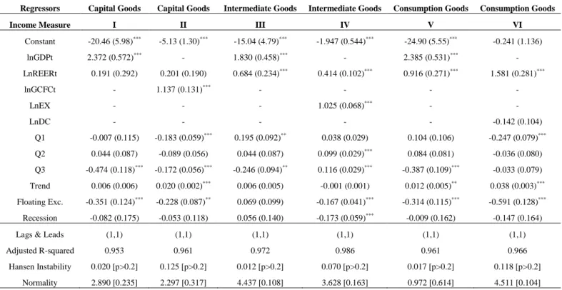
According to DOLS estimations in Table IV, the assumption of normally-disturbed error terms is satisfied. On the other hand, results from the parameter instability test of Hansen (1992) show that there is a stable parameter relationship among cointegrated variables. Results for capital goods from DOLS estimations suggest that long-run coefficient of REER is not statistically significant, and coefficient of GPD is elastic as 2.37. On the other hand, results from DOLS estimation suggest that insignificant coefficient of REER may come from the effect of the floating exchange rate regime and seasonality on capital goods imports. Results from DOLS estimation in Column II show that coefficient of REER is insignificant, and coefficient of GFCF is 1.13. The effects of seasonality, time trend and floating exchange rate regime are also significant. Negative effect of the floating exchange rate regime on capital goods imports find in both framework. The time trend positively affects the capital goods imports demand as it is expected.
Findings for intermediate goods from DOLS estimations in Table 4 suggest that the long-run coefficient of GPD is 1.83, and coefficient of REER is inelastic (0.68). On the other hand, results from DOLS estimation suggest that only the dummy variables of seasonality are statistically significant. Results in Column IV for intermediate goods also report that the coefficient of REER is 0.41, and the coefficient of exports is 1.02. Effects of seasonality, the great recession, and floating exchange rate regime are also significant variables. Negative effects of floating exchange rate regime and the great recession on intermediate goods imports are also valid in this framework for intermediate inputs imports.
Table IV. Results of the dynamic ordinary least square estimations
Regressors Capital Goods Capital Goods Intermediate Goods Intermediate Goods Consumption Goods Consumption Goods
Income Measure I II III IV V VI
Constant -20.46 (5.98)*** -5.13 (1.30)*** -15.04 (4.79)*** -1.947 (0.544)*** -24.90 (5.55)*** -0.241 (1.136) lnGDPt 2.372 (0.572)*** - 1.830 (0.458)*** - 2.385 (0.531)*** - LnREERt 0.191 (0.292) 0.201 (0.190) 0.684 (0.234)*** 0.414 (0.102)*** 0.916 (0.271)*** 1.581 (0.281)*** lnGCFCt - 1.137 (0.131)*** - - - - LnEX - - - 1.025 (0.068)*** - - LnDC - - - -0.142 (0.104) Q1 -0.007 (0.115) -0.183 (0.059)*** 0.195 (0.092)** 0.038 (0.029) 0.104 (0.106) -0.247 (0.079)*** Q2 0.044 (0.087) -0.089 (0.056) 0.044 (0.087) 0.099 (0.029)*** 0.084 (0.081) -0.036 (0.080) Q3 -0.474 (0.118)*** -0.172 (0.056)*** -0.246 (0.094)** 0.116 (0.029)*** -0.387 (0.109)*** -0.033 (0.079) Trend 0.006 (0.006) 0.020 (0.002)*** 0.006 (0.005) -0.001 (0.001) 0.012 (0.005)** 0.038 (0.003)*** Floating Exc. -0.351 (0.124)*** -0.228 (0.087)** 0.069 (0.099) -0.167 (0.041)*** -0.314 (0.115)*** -0.591 (0.128)*** Recession -0.082 (0.175) -0.053 (0.118) 0.056 (0.140) -0.173 (0.059)*** -0.009 (0.162) -0.147 (0.164)
Lags & Leads (1,1) (1,1) (1,1) (1,1) (1,1) (1,1)
Adjusted R-squared 0.953 0.961 0.972 0.986 0.961 0.966
Hansen Instability 0.020 [p>0.2] 0.125 [p>0.2] 0.012 [p>0.2] 0.070 [p>0.2] 0.017 [p>0.2] 0.118 [p>0.2] Normality 2.890 [0.235] 2.297 [0.317] 4.437 [0.108] 3.628 [0.163] 0.972 [0.614] 4.511 [0.104]
Notes: The coefficient covariance matrix is calculated by using Barlett Kernel and the bandwidth selection
method of Andrews (1991). Hansen instability refers to the LM statistic of Hansen (1992) parameter instability test that null hypothesis of series are cointegrated. Standard errors are given in parentheses and probability values are given in brackets. ***, ** and * indicate significance levels at the 1%, 5% and 10%, respectively.
Results in Column V for consumption goods imports suggest that the long-run coefficient of GPD is 2.38, and coefficient of REER is 0.91. Moreover, findings show that only the dummy variables of seasonality, time trend, and floating exchange rate regime are statistically significant. Once again, floating exchange rate regime negatively affected on consumption goods imports. Furthermore, time trend positively impacted on consumption goods imports. Results in Column VI report that coefficient of REER is elastic and 1.58, and the coefficient of domestic credits is statistically insignificant. Effects of seasonality, time trend, and floating exchange rate regime are also significant determinants. Negative effects of floating exchange rate regime and the great recession on consumption goods imports also exist in this framework for consumption goods imports. Finally, we report the summary of the long-run and the short-run results by ARDL and DOLS in Table V as follows:
Table V. Summary of the long-run and the short-run results
Long-run
BEC Classification GDP REER GFCF REER EX REER DC REER
Capital Goods Yes
Yes
(No in DOLS) Yes
Yes
(No in DOLS) - - - -
Intermediate Goods Yes Yes - - Yes Yes - -
Consumption Goods Yes Yes - - - - No Yes
Short-run
BEC Classification GDP REER GFCF REER EX REER DC REER
Capital Goods Yes Yes Yes Yes - - - -
Intermediate Goods Yes Yes - - Yes Yes - -
To sum up, empirical findings from ARDL models indicate that possible deprecation of the Turkish Lira limitedly increases all disaggregated import goods, and the biggest impact occurs on consumption goods imports both in the short and the long-run. Results from DOLS estimations for capital goods imports indicate that the parameter of REER is insignificant. At this point, we would like to emphasize that the effect of REER will be limited or temporary because we generally obtain inelastic coefficients. According to ARDL and DOLS estimations, GDP, as the main determinant of disaggregated imports demand, has the biggest impact on capital goods in the short-run and on consumption goods imports in the long-run.
4. Concluding Remarks
This paper estimates disaggregated import demand functions for Turkey, for the period from 1989 to 2012 in quarterly data set. We examine both the short-run and the long-run disaggregated import demand functions for capital goods, intermediate inputs, and consumption goods by using ARDL model and DOLS estimation technique. Besides GDP and REER; the impacts of seasonality, time trend, the periods of floating exchange regime, and the great global recession are also taken into account in the estimations of disaggregated import demand functions.
In this paper, four main conclusions stand out. First, both short-run elasticity and long-run elasticity of domestic demand are higher than real exchange rate in all statistically significant cases. These findings are in the line with previous researches of Togan and Berument (2007) and Aldan et al. (2012). One should however recall that Togan and Berument (2007) analyzed only the long-run, while Aldan et al. (2012) analyzed only the short-run dynamics of disaggregated import demands in Turkey. Second, we find that the short-run coefficient of domestic demand is greater in capital goods imports, compared to consumption goods and intermediate goods import demands. On the other hand, the short-run coefficient of real exchange rate is greater in consumption goods imports as compared to other disaggregated import demands. Third, results from ARDL model and DOLS technique both indicate that long-run coefficients of domestic demand is greater in consumption goods imports as compared to other disaggregated import demands. Also, long-run coefficients of real exchange rate are greater in consumption goods imports as compared to other disaggregated import demands. Fourth, we realize the significant effects of floating exchange rate regime on capital goods and consumption goods imports in the long-run. We also find the significant effects of seasonality on all disaggregated import demands cases, whereas time trend and the great recession have almost no impact on disaggregated import demands in Turkey.
All empirical findings show that possible deprecation of the TRY has limited effects on imports demand. The biggest impact of REER occurs on consumption goods. However, the share of consumption goods imports in total imports is less than 13%. Therefore, deprecation of the TRY would not have a significant effect in general on the import demand of Turkey. Accordingly, the main determinant of import demand in Turkey is GDP. However, in order to get more detailed concluding remarks, the demand elasticity of exports should also be examined. Thus, we can take into account the Marshall-Lerner condition as well.
References
Aldan, A., I. Bozok and M. Gunay (2012) “Short Run Import Dynamics of Turkey” Central Bank of the Republic of Turkey working paper number 12/25.
Andrews, D. W. K. (1991) “Heteroskedasticity and Autocorrelation Consistent Covariance Matrix Estimation” Econometrica 59, 817-58.
Aydin, F., U. Ciplak and M. E. Yucel (2004) “Export Supply and Import Demand Models for the Turkish Economy” Central Bank of the Republic of Turkey working paper number 04/09. Bahmani-Oskooee, M. and O. Kara (2005) “Income and Price Elasticities of Trade: Some New Estimates” International Trade Journal 19, 165-78.
Cheung, Y., M. D. Chinn and X. W. Qian (2012) “Are Chinese Trade Flows Different?”
Journal of International Money and Finance 31, 2127-46.
Fukumoto, M. (2012) “Estimation of China's Disaggregate Import Demand Functions” China
Economic Review 23, 434-44.
Goldstein, M. and M. Khan (1985) “Income and Price Effect in Foreign Trade” in Handbook
of International Economics by R.W. Jones and P.B. Kenen, Eds., North Holland: Amsterdam,
1042-99.
Gopinath, G., O. Itskhoki and B. Neiman (2012) “Trade Prices and the Global Trade Collapse of 2008-09” IMF Economic Review 60, 303-28.
Gozgor, G. (2011) “Purchasing Power Parity Hypothesis among the Main Trading Partners of Turkey” Economics Bulletin 31, 1432-38.
Hansen, B. E. (1992) “Tests for Parameter Instability in Regressions with I(1) Processes”
Journal of Business and Economic Statistics 10, 321-35.
Inder, B. (1993) “Estimating Long-run Relationships in Economics: A Comparison of Different Approaches” Journal of Econometrics 57, 53-68.
Johansen, S. (1988) “Statistical Analysis of Cointegration Vectors” Journal of Economic
Dynamics and Control 12, 231-54.
Johansen, S. (1991) “Estimation and Hypothesis Testing of Cointegration Vectors in Gaussian Vector Autoregressive Models” Econometrica 59, 1551-80.
Johansen, S. and K. Juselius (1990) “Maximum Likelihood Estimation and Inference on Cointegration with Applications to the Demand for Money” Oxford Bulletin of Economics
and Statistics 52, 169-210.
Ketenci, N. and I. Uz (2010) “Trade in Services: The Elasticity Approach for the Case of Turkey” International Trade Journal 24, 261-97.
Khan, M. (1975) “The Structure and Behavior of Imports of Venezuela” Review of
Economics and Statistics 57, 221-24.
Kotan, Z. and M. Saygili (1999) “Estimating an Import Function for Turkey” Central Bank of the Republic of Turkey discussion paper number 9909.
Mah, J. S. (2000) “An Empirical Examination of the Disaggregated Import Demand of Korea-the Case of Information Technology Products” Journal of Asian Economics 11, 237-44.
Montalvo, J. G. (1995) “Comparing Cointegrating Regression Estimators: Some Additional Monte Carlo Results” Economics Letters 48, 229-34.
Park, J. Y. (1992) “Canonical Cointegrating Regressions” Econometrica 60, 119-43.
Pattichis, C. A. (1999) “Price and Income Elasticities of Disaggregated Import Demand: Results from UECMs and an Application” Applied Economics 31, 1061-71.
Pesaran, M. H. and Y. Shin (1999) “An Autoregressive Distributed Lag Modeling Approach to Cointegration Analysis” in Econometrics and Economic Theory in the 20th Century: The Ragnar Frisch Centennial Symposium by S. Strom Eds., Cambridge University Press:
Cambridge, 371-413.
Pesaran, M. H., Y. Shin and R. J. Smith (2001) “Bounds Testing Approaches to the Analysis of Level Relationships” Journal of Applied Econometrics 16, 289-326.
Phillips, P. C. B. and B. E. Hansen (1990) “Statistical Inference in Instrumental Variables Regression with I(1) Processes” Review of Economic Studies 57, 99-125.
Phillips, P. C. B. and P. Perron (1988) “Testing for a Unit Root in Time Series Regression”
Biometrika 75, 335-46.
Saikkonen, P. (1992) “Estimation and Testing of Cointegrated Systems by an Autoregressive Approximation” Econometric Theory 8, 1-27.
Senhadji, A. (1998) “Time-series Estimation of Structural Import Demand Equations: A Cross-country Analysis” IMF Staff Papers 45, 236-88.
Stock, J. H. and M. Watson (1993) “A Simple Estimator of Cointegrating Vectors in Higher Order Integrated Systems” Econometrica 61, 783-820.
Togan, S. and H. Berument (2007) “The Turkish Current Account, Real Exchange Rate and Sustainability: A Methodological Framework” Journal of International Trade and Diplomacy
1, 155-92.
Wang, Y. H. and J. D. Lee (2012) “Estimating the Import Demand Function for China”
Economic Modelling 29, 2591-96.
Yavuz, N. C. and B. Guris (2006) “An Aggregate Import Demand Function for Turkey: The Bounds Testing Approach” METU Studies in Development 33, 311-25.
Yin, F. and S. Hamori (2011) “Estimating the Import Demand Function in the Autoregressive Distributed Lag Framework: The Case of China” Economics Bulletin 31, 1576-91.
Zivot, E. and D. W. K. Andrews (1992) “Further Evidence on the Great Crash, the Oil-price Shock, and the Unit-root Hypothesis” Journal of Business and Economic Statistics 10, 251-70.