Threshold Regression Model for Taylor Rule: The Case of
Turkey
PINAR DENIZ
∗Marmara University
THANASIS STENGOS
†University of Guelph
EGE YAZGAN
‡Istanbul Bilgi University
This paper employs the structural threshold approach of Kourtellos et al. (2016) to examine
various specifications of the Taylor rule model. Contrary to the previous work on the Taylor
rule, this methodology allows for endogeneity of the threshold variable in addition to the
right-hand-side variables suggesting a fully comprehensive flexible framework that does
not rely on restrictive linearity and/or exogeneity assumptions. In order to examine the
model, Turkey is selected as an inflation targeting developing economy, since its central
bank (the Central Bank of Turkey) as argued by Dincer and Eichengreen (2014) has been
one of the fastest improving central banks in terms of its transparency score. We will use
monthly data for the period of 2004-2018 that includes a number of historical episodes
such as the global financial crisis as well as various internal political developments that
may have had an impact on the fluctuations of the relevant macroeconomic variables as
well as on the functional form of the inflation targeting Taylor rule specification. Empirical
findings highlight the different reactions of the central bank in determining policy rate
under different regimes.
Keywords:
Nonlinearities, Taylor rule, Threshold regression models
JEL Classifications:
C26, E52, E58
∗
[email protected], Marmara niversitesi Gztepe YerleÅkesi, 34722 Kadky,
stanbul
†
[email protected], 50 Stone Road East Guelph, Ontario, Canada N1G 2W1
‡[email protected], Kazm Karabekir Cad.
No:
2/13, 34060, Eypsultan,
stanbul
c
2020 Pinar Deniz, Thanasis Stengos, and Ege Yazgan.
Licenced under the Creative Commons
Attribution-Noncommercial 3.0 Licence (http://creativecommons.org/licenses/by-nc/3.0/).
Available at http://rofea.org.
1
Introduction
The Turkish economy has had a long history of high inflation, even reaching levels of over a
hundred percent, combined with successive periods of economic crises in 1979, 1994, 1997 and
2001. After the decades of high inflation, Central Bank of the Republic Turkey (CBRT) was
o
fficially granted its independence following the amendment of the Central Bank Law in 2001
and started to implement implicit inflation targeting (IT) policies. Following a successful
disin-flation effort which managed to bring down the indisin-flation rate to single digits, IT was explicitly
adopted as the main target policy. As a result CBRT gained credibility and found itself among
the top central banks in terms of its rapid increase in the transparency index achieved. Within
the group of over 120 central banks CBRT’s transparency score rose from 3.2 in 1998 to 5.5 in
2010 (Dincer and Eichengreen, 2014). The success of this disinflation e
ffort
1led researchers
to estimate di
fferent Taylor rule models for Turkey (Us, 2007; Yazgan and Yilmazkuday, 2007;
C
¸ a˘glayan and Astar, 2010; Aklan and Nargelecekenler, 2008; Civcir and Akc¸a˘glayan, 2010;
Khakimov et al., 2010; Erdem and Kayhan, 2011; G¨uney, 2016). These studies provided
differ-ent results for the estimated parameters as they consider di
fferent periods, versions of the rule
and different methodologies.
Following the great financial crisis 2009, the monetary policy of CBRT has been gradually
redesigned and a macroprudential policy approach has become more and more dominant (Kara,
2012, 2016). This redesign in the monetary policy approach has raised some concerns regarding
the loss of the main objective of maintaining price stability. G¨urkaynak et al. (2015) stated that
while CBRT was a strong inflation targeter early in 2000’s, it has began to pay less attention to
inflation after 2009. They also provided empirical evidence to their claim by detecting a change
in the estimated policy rule coe
fficient at that date. From the institutional perspective Ozel,
2012 indicated a deterioration in the independence of Turkish regulatory agencies in general,
including the CBRT, even though they were regarded as a model for a number of countries at
the begining of 2000’s. Similarly Demiralp and Demiralp (2019) pointed out that CBRT has
currently been experiencing an erosion in its independence. They showed that political
inter-vention, as captured by political commentaries favoring a drop in interest rates, is as influential
as traditional variables in the Taylor rule.
These policy changes and concerns of political interventions indicates the importance of
in-troducing non-linearities and regime changes in modeling Taylor rule targeting for Turkey. This
topic has been recently analyzed together with some other emerging market countries by
Capo-rale et al. (2018) via a threshold model using the inflation as a threshold variable. In this paper,
we also analyze the Taylor rule targeting of Turkey via threshold models allowing however
for the threshold variable and the regressors to be endogenous. In the literature of nonlinear
regression models, threshold regression o
ffers a convenient and parsimonious way to
terize nonlinearities without running into curse of dimensionality issues that plague alternative
nonparametric and semiparametric approaches. These models imply that below and under the
estimated threshold parameter, the slope parameters di
ffer and imply regime specific marginal
responses. Initial studies based on the work of Hansen (2000) and Caner and Hansen (2004),
even allowing for endogenous regressors, assume that the threshold variable itself is exogenous.
The structural threshold models by Kourtellos et al. (2016) provides a generalization that allows
for the endogeneity for the threshold variable and also regime-specific heteroscedasticity. In this
paper we will follow their approach as our estimation strategy, since the threshold variable may
be in itself an important determinant that cannot be separated in an ad hoc manner from the
other potentially endogenous regressors.
The rest of the study is organized as follows. Section 2 explains the model, data and
method-ology. Section 3 presents the empirical findings, while the last section concludes the paper. In
the appendix we collect a variety of additional Taylor rule specifications that were estimated in
addition to the ones reported in the main text
2. These different specifications confirm the main
features of the models presented in the main body of the paper.
2
Model and methodology
The Taylor rule suggests a basic monetary policy rule
3for central banks such that inflation
and real output deviations from their target levels would be determining the short-term interest
rate target. Following this basic rule, several different versions are used in the literature taking
into account open economy requirements and country specifications. We consider two di
fferent
specification for the Taylor rule.
2.1
Model I
This first model is a basic Taylor rule augmented by exchange rate. The standard Taylor rule
(Taylor, 1993) observes a policy rule for Federal Reserve suggesting that inflation gap and
output gap are the determinants of the federal funds rate. Several papers considered the
in-corporation of exchange rate as an additional variable into the policy rule (see, among others,
Taylor (2001) and Mohanty and Klau (2005)). Many studies of Turkish monetary policy
high-2In the literature, there are many criticisms against different specifications. Hamilton (2018) criticizes
HP filtering technique for calculations of gap. Fernandez et al. (2010) suggests that unemployment rate
is more useful than detrended output in the monetary policy models. Orphanides (2003) argues that
concepts such as the natural rate of interest and potential output are known to be notoriously unreliable as
policy indicators. Yellen (2005) criticizes constant natural (or neutral) real interest rate. Considering these
criticisms, we run several Taylor rule estimations using di
fferent specifications for relevant variables. We
do not document all the results to conserve some space, however, the complete results can be provided
upon request.
3
Taylor (1993) provides a policy rule for Federal Reserve suggesting that inflation (π) above a target of 2
percent and percentage deviation of real GDP from its trend (y) affect federal funds rate (r) by 0.5, i.e.,
r
= π + 0.5y + 0.5(π − 2) + 2.
light the importance of the inclusion of exchange rate in the policy rule considering the fragility
of economy to exchange rate shocks (Us, 2007; Civcir and Akc¸a˘glayan, 2010; Erdem and
Kay-han, 2011). Moreover, Turkey was found as the only country whose reaction function has a
significant response to exchange rate changes among the 5 emerging markets considered by
Caporale et al. (2018, pp.312). Following this literature, the first estimated Taylor rule in this
paper also includes an exchange rate variable in addition to inflation gap and output gap. Froyen
and Guender (2018) strongly suggest the use of real exchange rate in a Taylor rule specification
and following this suggestion, we will use the real exchange rate rather than the nominal one.
The model employs policy rate (i
t) as a function of inflation gap, which is the difference
between realized inflation (π
t) and the inflation target set by the central bank (π
Tt), output gap
( ˜
y
t), which is calculated as HP filtered output, and the real e
ffective exchange rate (rer
t).
i
t= β
0+ β
1(π
t−
π
tT)
+ β
2y
˜
t+ β
3rer
t(1)
2.2
Model II
The second model is selected based on CBRT’s own approach to be country specific, as outlined
in inflation reports of CBRT (CBRT, 2018). This model takes the natural real interest rate into
account:
r
t= r
t−1∗+ ρ
r(r
t−1− r
∗t−1)
+ (1 − ρ
r)(θ
πE
t(π
t+1−
π
Tt)
+ θ
yy
˜
t)
+ u
t(2)
where ˜
y
tis the output gap using HP filter, r
tis the interest rate minus the average inflation rate
and r
∗is the natural (neutral) real interest rate.
2.3
Methodology
In this study, the two Taylor rule models outlined above are examined using a threshold
regres-sion methodology, an approach that relies on a parsimonious modeling of possible nonlinearities
that avoids the curse of dimensionality issue that plagues alternative nonparametric
methodolo-gies. Threshold regression models have been used extensively in applied work in the last twenty
years. In the first generation of threshold models, Hansen (2000) developed a useful asymptotic
distribution theory for both the threshold parameter estimate and the regression slope
coeffi-cients under the assumption that the threshold e
ffect becomes smaller as the sample increases,
while Caner and Hansen (2004) allowed for endogenous regressors, under an exogenous
thresh-old variable framework. In the second generation of threshthresh-old models Kourtellos et al. (2016)
allow for an endogenous threshold variable. The main strategy here was to exploit the intuition
obtained from the limited dependent variable literature, and to relate the problem of having an
endogenous threshold variable with the analogous problem of having an endogenous dummy
variable or sample selection in the limited dependent variable framework. However, there is one
important di
fference. While in sample selection models, we observe the assignment of
obser-vations into regimes but the (threshold) variable that drives this assignment is taken to be latent,
here, it is the opposite here as we do not know which observations belong to which regime
(we do not know the threshold value), but we can observe the threshold variable. To put it
dif-ferently, while endogenous dummy models treat the threshold variable as unobserved and the
sample split as observed (dummy), here one treats the sample split value as an unknown to be
estimated. Just as in the limited dependent variable framework, consistent estimation of slope
parameters under normality requires the inclusion of a set of inverse Mills ratio bias
correc-tion terms, implying that the slope parameter estimates of the threshold regression by Hansen
(2000) and Caner and Hansen (2004) will be inconsistent in the endogenous threshold variable
case due to the omission of the inverse Mills ratio bias correction terms.
As there are many potential endogenous threshold variable candidates we select the one that
best fits the data using a GMM J-statistic criterion to identify the best threshold model out of
the pool of threshold variable candidates. Once the threshold variable is selected then we will
adopt both a two stage least squares (2SLS) and GMM estimation approach for the estimation
of slope parameters and we will also provide asymptotically valid confidence intervals for the
threshold parameter. We will proceed as follows. We first test the null hypothesis of linearity
against the alternative of a nonlinear Taylor rule model using the LM-test of Hansen (2000)
for all possible threshold variable candidates and select the one with the best fit according to
the J-statistic. We then estimate the threshold Taylor rule models, by applying the Kourtellos
et al. (2016) structural threshold regression (STR) estimation tests using both two-stages least
squares and GMM methodology.
3
Empirical Findings
3.1
Data
We employ monthly data for the period of 2004-2018 for Turkey. The existence of a ”plethora”
of interest rates employed by CBRT (see Figure 1) requires a choice on the appropriate policy
rate. We use official policy rates, i.e., overnight rate for the period of January 2004 - 2010
April, one-week repo for the period of May 2010 - December 2013 and average funding rate of
CBRT
4for the period of January 2014 - June 2018.
5Inflation is used as the annual (%) change of CPI. Inflation target is the o
fficial target of
CBRT. Output is seasonally adjusted industrial production index. Output gap is calculated by
taking HP filter of logarithmic output. Real e
ffective exchange rate (RER) is CPI 2003 based
4This is the weighted average cost of outstanding funding by the CBRT via Interbank Money Market
(overnight lending facility) and Open Market Operations (BIST repo, primary dealer repo, one-week repo
via quantity auction, one-week repo via traditional auction and one-month repo, see K¨uc¸¨uk et al. (2016)
5Alp et al. (2012) and G¨urkaynak et al. (2015), both use TRlibor arguing that it is a better predictor as a
policy rate.
Figure 1: Policy rates (%)
and is in logarithmic form. A rise in RER refers to appreciation.
6Table 1 presents descriptive
statistics.
Table 1: Descriptive statistics
Variables Mean Std Dev Max Min Interest rate 0.1299 0.0681 0.3100 0.0500 Inflation rate 0.0874 0.0199 0.1600 0.0400 Inflation gap 0.0235 0.0220 0.0781 -0.0240 Output gap 0.0003 0.0415 0.0900 -0.1500 RER 4.6697 0.1031 4.8514 4.3442
Table 2 provides Phillips and Perron (1988) and Lee and Strazicich (2003) unit root test
results. The latter one allows for breaks with unknown dates. Inflation gap, output gap and
real exchange rate are observed to be stationary rejecting the null hypothesis of unit root with
break. However, the interest rate produces an ambiguous result with either test. There are
several studies observing an ambiguity regarding the (non)stationarity property of interest rates
but end up using them in levels according to theoretical arguments Clarida et al. (2000); Martin
and Milas (2004, 2013); Castro (2011); Caporale et al. (2018).
6
CBRT defines real effective exchange rate, which is calculated by the weighted averages of foreign
currencies according to their trade ratio, using this formula: P/(P
∗XR), where P and P
∗are domestic and
foreign prices, respectively.
Table 2: Unit Root Tests
Phillips-Perron Test Lee-Strazizich Test Variables C C-T LM-Stat Break date Interest rate -2.6030* -0.7824 -2.9339 2014M08 Inflation gap -1.8450 -0.7889 -4.3916** 2008M09 Output gap -4.7449*** -4.7317*** -4.3922** 2008M09 RER -0.5711 -2.0608 -4.2337** 2008M09
Note: The values above are test statistics. The null hypothesis for Phillips-Perron and Lee-Strazizich tests are existence of unit root (with break in the latter one). *,**,*** denote significance at 10%,5% and 1% significance levels. For Lee-Strazizich test, the critical values for RER are 4.7833, 4.2337 and 3.9588; for the other variables are -4.7266, -4.1707 and -3.8877 at 1%, 5% and 10% significance levels, successively. For Phillips-Perron test, the critical values are -2.5757, -2.8781 and -3.4683 for constant case; -3.1421, -3.4360 and -4.0119 for constant and trend case, successively. C and C-T refer to constant and constant&trend cases.
3.2
Structural Threshold Taylor Rule model I
In this first model, nominal interest rate is used in levels form and is regressed on inflation
gap, output gap and real e
ffective exchange rate using each variable as a candidate threshold
variable. q
tis defined as the threshold variable and γ is the threshold parameter. Threshold
variable lower
/higher than the estimate for the threshold parameter denotes low regime (L)
periods
/high regime (H) periods.
i
t= I(q
t≤
γ)(β
L0+ β
L 1(π
t−
π
Tt)
+ β
L 2y
˜
t+ β
L3rer
t+ I(q
t> γ)(β
H0+ β
H 1(π
t−
π
Tt)
+ β
H 2y
˜
t+ β
3Hrer
t)
+ u
t. (3)
Hansen (2000) LM-test in Table 3 shows that regressions with all candidate threshold
vari-ables reject the null hypothesis of linearity for model I. The Structural Threshold Taylor Rule
(STR) model using GMM estimation shows that regression with the threshold variable inflation
gap best fits as the J statistic is the lowest. However, the threshold estimate is observed to be
insignificant which results in ambiguity in terms of selecting the best fitted model. There are
two models with significant threshold parameters, RER and interest rate. Among these two
candidates, RER has the smallest J-statistics. Hence, in Table 4, test results for the model with
the threshold variable RER are provided for Hansen, STR-GMM and STR-2SLS
7.
The test results reflects that in the low regime period, when RER is lower than the estimated
threshold level, inflation gap and RER variables are found to be significant with negative coe
ffi-cients. Keeping in mind that a rise in RER refers to an appreciation, the low regime period refers
to the relatively depreciated currency period and the negative coe
fficient of RER suggests that
7Test results for the models with other threshold candidates are available in the appendix
Table 3: Threshold estimates for Model 1
Threshold Hansen Test GMM 2SLS
Candidates LM-test Threshold J-stat Threshold Threshold Inflation gap 48.2661 0.0039 4.5242 -0.0017 0.0039 (0.0000) [-0.0001, 0.0070] [-0.0151, 0.062] [-0.0151, 0.062] Output gap 36.7058 0.0112 22.5194 0.0000 0.0100 (0.0000) [0.0056, 0.0249] [-0.05, 0.05] [-0.05, 0.05] RER 32.2128 4.6619 8.5986 4.6687 4.7005 (0.0000) [4.6283, 4.7101] [4.5096, 4.7878] [4.5096, 4.7878] Interest rate 115.8041 0.1550 25.9689 0.1400 0.1400 (0.0000) [0.1350, 0.1550] [0.06, 0.23] [0.06, 0.23]
Note: Apart from LM-test and J statistics, values above are threshold estimates. Values in brackets are confidence intervals in 95%. Values in paranthesis for LM-test are bootstrap p-values.
a depreciation in the currency raises interest rates in this period. As will be discussed below,
since depreciations not only induce serious cost inflation in Turkey but also cause
inflation-ary expectations to become more pessimistic, CBRT is expected to have tendency to favor the
appreciation. As an emerging market country raising interest rates may help to attract capital
flows, hence results in appreciation which is also helpful for controlling prices. On the other
hand, the inflation gap is observed to have a negative e
ffect on interest rate contrary to theory.
Hence, we may argue that when the depreciation is over the threshold, concerns on currency
dominate monetary policy over inflation targeting and we observe an opposite sign on the
infla-tion gap variable. However, in the high regime period, that is when RER is above the estimated
threshold level for RER (appreciated currency), the inflation gap becomes the sole significant
variable with the expected sign. In this period, there is no need for CBRT to worry about
de-preciation for its adverse e
ffect on inflation so it can use its interest rate policy to dampen the
domestic demand to fight against inflation.
3.3
Structural Threshold Taylor Rule model II
In this model, the natural real interest rate (r
∗t) is estimated using Kalman filter based on ¨
O˘g¨unc¸
and Batmaz (2011).
8In our model, expected inflation is the expected end of year inflation and
real exchange rate is also added to the original model in equation 2 considering the importance
of exchange rate to a developing open economy.
r
t− r
∗t−1
= I(q
t≤
γ)(β
L0+ β
L1(r
t−1− r
∗t−1)
+ β
L2(E
tπ
end−
π
Tt)
+ β
3Ly
˜
t+ β
L4rer
t)
+ I(q
t> γ)(β
H0+ β
1H(r
t−1− r
∗t−1)
+ β
H2(E
tπ
end−
π
Tt)
+ β
H3y
˜
t+ β
H4rer
t)
+ u
t(4)
8
They employ two alternative specifications for natural real interest rates for the period of 1989-2005.
The first model assumes a simple random walk specification for natural interest rate and the second
model related natural rate with a trend growth rate and risk premium. Kara et al. (2007) also make a
similar proposition to the first model in their output gap model estimation. For simplicity, we employ the
first model of ¨
O˘g¨unc¸ and Batmaz (2011)
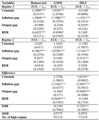
Table 4: Threshold Test Results for Model 1
Variables Hansen test GMM 2SLS Regime 1 RERt< ˆγrer RERt< ˆγrer RERt< ˆγrer
Constant 2.1800*** 3.8181** -0.3148 (0.5137) (1.6786) (0.8098) Inflation gap -1.3848*** -2.1986*** -1.1553*** (0.3128) (0.3555) (0.3415) Output gap -0.2996 -0.2348 -0.2519* (0.2292) (0.227) (0.142) RER -0.4422*** -0.8306* 0.2189 (0.1111) (0.4785) (0.2276) Regime 2 RERt> ˆγrer RERt> ˆγrer RERt> ˆγrer
Constant 0.225 1.4425 -2.1362 (0.617) (3.035) (1.3057) Inflation gap 0.7483*** 1.0198*** 1.1144*** (0.2334) (0.2368) (0.1916) Output gap 0.2077 0.1495 0.3131** (0.1389) (0.1610) (0.1260) RER -0.0218 -0.2457 0.3558 (0.1302) (0.5323) (0.2278) Difference Constant 2.3756 1.8214** (1.5863) (0.9042) Inflation gap -3.2184*** -2.2697*** (0.4377) (0.3913) Output gap -0.3842 -0.5650*** (0.277) (0.1908) RER -0.5849*** -0.1369 (0.1953) (0.1754) IMR -0.2191 0.7251** (0.7092) (0.3607) JSSE 0.5775 0.5872
No. of high regime 97/174 77/174
Note: The instrumental variables for the model are first and twelfth lags of inflation gap, output gap and real exchange rate. Values in paranthesis are standard errors. *,**,*** denote significance at 10%,5% and 1% significance levels. JSSE refers to joint sum of squares and IMR refers to inverse Mill ratio.
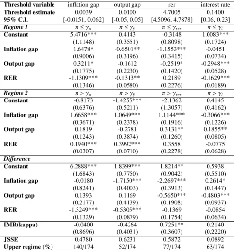
Hansen (2000) LM-test in Table 5 shows that models with all the threshold candidates reject
the null of linearity at 10% significance level. The STR model using GMM selects the model
with the threshold variable output gap according to J-statistics, however the threshold estimate
is observed to insignificant. Again, only the model with RER as the threshold variable has
significant threshold effect.
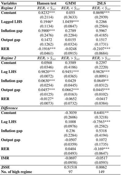
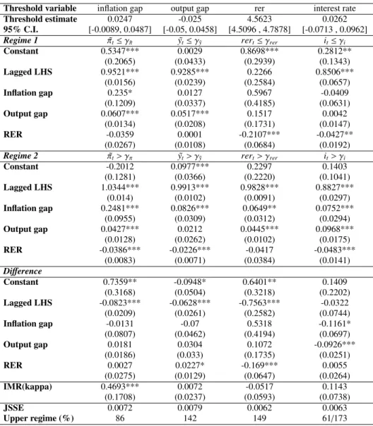
The test results for Model 2, given in Table 6 are in line with the results in Model 1, such that
RER has a negative effect in the low regime period (depreciated currency), whereas inflation
gap has a positive e
ffect on the real policy rate gap (using natural real policy rate) in the high
regime period (appreciated currency). In addition to these findings, Model 2 shows a positive
effect of output gap in the appreciated currency period. Hence, the high regime period fits the
Table 5: Threshold estimates for Model 2
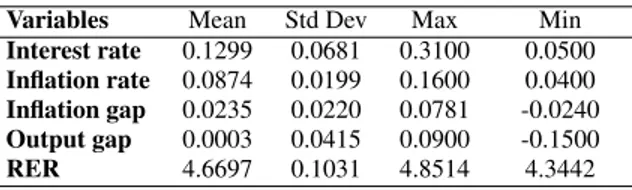
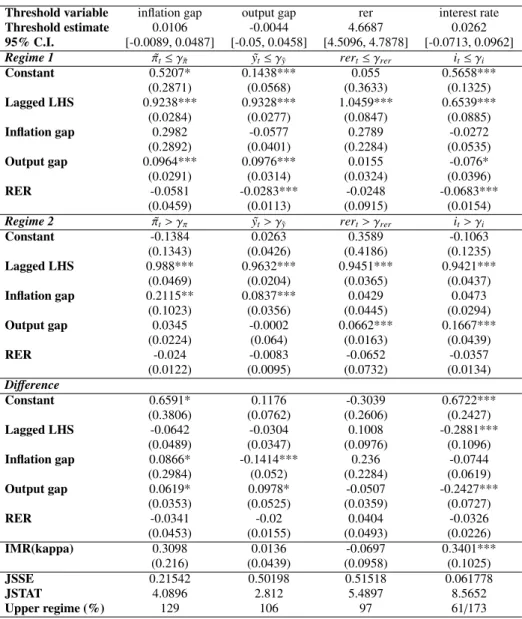
Threshold Hansen Test GMM 2SLS
Candidates LM-test Threshold J-stat Threshold Threshold Inflation gap 14.3985 0.0478 4.0896 0.0106 0.0247 (0.033) [0.0170, 0.0574] [-0.0089, 0.0487] [-0.0089, 0.0487] Output gap 13.0258 -0.024 2.812 -0.0044 -0.0250 (0.065) [0.034, 0.0200] [-0.05, 0.0458] [-0.05, 0.0458] RER 17.3548 4.5623 5.4897 4.6687 4.5623 (0.005) [0.5622, 4.5886] [4.5096, 4.7878] [4.5096 , 4.7878] Interest rate 21.781 0.0662 8.5652 0.0262 0.0262 (0.001) [0.0061, 0.0711] [-0.0713, 0.0962] [-0.0713 , 0.0962] Note: As in Table 3
expectations from a standard central bank policy standpoint as both the inflation and output
gaps display positive and significant effects.
4
Conclusion
This study examines how policy rate is determined in Turkish economy using two Taylor rule
models. As an open developing economy, it seems highly possible that there is not a single
rule followed by CBRT as also argued by several empirical work in the literature (Kara et al.,
2007; G¨urkaynak et al., 2015; Caporale et al., 2018). Dummy variables, structural breaks,
sam-ple splitting models are some of the options to handle nonlinearity issues. However, threshold
regression models stand out since these techniques estimate the threshold parameters and hence
are less restrictive compared to time-dependent regime switching models. Kourtellos et al.
(2016), di
fferently from the previous threshold models, allows for endogeneity for the
thresh-old variables. In this paper, we employ GMM and two stages least squares methodology of
Kourtellos et al. (2016).
In the empirical work, real exchange rate is added to the standard Taylor rule model and
is selected as the preferred threshold variable by the employed test statistics. Our estimates
indicate the Taylor rule implies di
fferent behaviors according to whether the real exchange is
above or below the threshold. In the appreciated currency period, when CBRT has no need
to have concerns on currency due its adverse e
ffects on inflation, the Taylor rule exhibits its
expected characteristics and indicates that CBRT adjust interest rate according to inflation and
output.
However, in the times of currency depreciation, CBRT may appear to lose its main policy
objective of inflation targeting and focuses on the depreciation of the currency. We think that
this interpretation should be taken with caution. It is widely known that Turkish economy is
highly dependent on imported inputs and exchange rate depreciations cause to inflation via
pass-through mechanism. Moreover, currency depreciations deteriorate confidence, worsen inflation
expectations, and have the potential of leading to depreciation-inflation spiral (Arbalı, 2003;
Table 6: Threshold Test Results for Model 2
Variables Hansen test GMM 2SLS Regime 1 RERt< ˆγrer RERt< ˆγrer RERt< ˆγrer
Constant 0.8232*** 0.055 0.8698*** (0.2114) (0.3633) (0.2939) Lagged LHS 0.1946* 1.0459*** 0.2266 (0.1134) (0.0847) (0.2584) Inflation gap 0.5900*** 0.2789 0.5967 (0.2476) (0.2284) (0.4185) Output gap 0.1472 0.0155 0.1517 (0.1262) (0.0324) (0.1731) RER -0.1916*** -0.0248 -0.2107*** (0.0461) (0.0915) (0.0684) Regime 2 RERt> ˆγrer RERt> ˆγrer RERt> ˆγrer
Constant 0.0568 0.3589 0.2297 (0.0346) (0.4186) (0.2220) Lag LHS 0.9820*** 0.9451*** 0.9828*** (0.0072) (0.0365) (0.0091) Inflation gap 0.0630*** 0.0429 0.0649** (0.0254) (0.0445) (0.0312) Output gap 0.0457*** 0.0662*** 0.0445*** (0.0125) (0.0163) (0.0102) RER -0.0127* -0.0652 -0.0417 (0.0073) (0.0732) (0.0384) Difference Constant -0.3039 0.6401** (0.2606) (0.3218) Lag LHS 0.1008 -0.7563*** (0.0976) (0.2582) Inflation gap 0.236 0.5318 (0.2284) (0.4194) Output gap -0.0507 0.1072 (0.0359) (0.1735) RER 0.0404 -0.169*** (0.0493) (0.0647) IMR -0.0697 -0.0517 (0.0958) (0.0593) JSSE 0.51518 0.0062
No. of high regime 97 149
Note: As in Table 4. Lagged LHS refers to the lagged value of left hand side (dependent) variable variable.
Kara et al., 2007; Kara and ¨
O˘g¨unc¸, 2008; Karag¨oz et al., 2016; Civcir and Akc¸a˘glayan, 2010;
L´opez-Villavicencio and Mignon, 2017). As emphasized by Benlialper and C¨omert (2015),
because of its impact on inflation, exchange rate appreciation has played an important role as a
dis-inflationary tool in Turkey. Hence focusing on the currency depreciation may not necessary
mean that CBRT loses its objective of fighting inflation. As indicated in the introduction, after
the great financial crisis of 2009, the newly adopted macro-prudential approach has rendered
Turkish central bank more cautious about financial stability. As in many emerging markets, in
Turkey, financial stability is always considered closely linked to exchange rate stability. By also
following the famous fear of floating argument of Calvo and Reinhart (2002) it can be argued
that keeping exchange rate stable is crucial since fluctuations can deteriorate the confidence on
the economy leading to capital outflows that further destabilize exchange rates which hampers
the implementation of inflation targeting. Consequently, when the currency depreciation is
above certain threshold it is certainly possible that its priority dominates monetary policy.
References
Aklan, N. A. and Nargelecekenler, M. (2008), Taylor rule in practice: Evidence from Turkey,
International Advances in Economic Research 14(2), 156–166.
Alp, H., Ogunc, F. and Sarikaya, C. (2012), Monetary Policy and Output Gap : Mind the
Composition, CBT Research Notes in Economics No: 1207, Central Bank of the Republic
of Turkey.
Arbalı, E. C. (2003), Exchange Rate Pass-Through In Turkey: Looking for Asymmetries.,
Cen-tral Bank Review 3(2), 85–124.
Benlialper, A. and C¨omert, H. (2015), Implicit asymmetric exchange rate peg under inflation
targeting regimes: the case of Turkey, Cambridge Journal of Economics 40(6), 1553–1580.
C
¸ a˘glayan, E. and Astar, M. (2010), Taylor Rule: Is it an Applicable Guide for Inflation Targeting
Countries, Journal of Money Investment and Banking 18, 55–67.
Calvo, G. A. and Reinhart, C. M. (2002), Fear of floating, The Quarterly Journal of Economics
117(2), 379–408.
Caner, M. and Hansen, B. E. (2004), Instrumental variable estimation of a threshold model,
Econometric Theory 20(5), 813–843.
Caporale, G. M., Helmi, M. H., C
¸ atık, A. N., Ali, F. M. and Akdeniz, C. (2018), Monetary
policy rules in emerging countries: Is there an augmented nonlinear taylor rule?, Economic
Modelling 72, 306–319.
Castro, V. (2011), Can central banks monetary policy be described by a linear (augmented)
Taylor rule or by a nonlinear rule?, Journal of Financial Stability 7(4), 228–246.
CBRT (2018), Central Bank of the Republic of Turkey, Inflation Report 2018-III.
Civcir, I. and Akc¸a˘glayan, A. (2010), Inflation targeting and the exchange rate: Does it matter
in Turkey?, Journal of Policy Modeling 32(3), 339–354.
Clarida, R., Gali, J. and Gertler, M. (2000), Monetary policy rules and macroeconomic stability:
evidence and some theory, The Quarterly Journal of Economics 115(1), 147–180.
Demiralp, S. and Demiralp, S. (2019), Erosion of Central Bank Independence in Turkey, Turkish
Studies 20(1), 49–68.
Dincer, N. N. and Eichengreen, B. (2014), Central bank transparency and independence:
up-dates and new measures, International Journal of Central Banking 10(1), 189–253.
Erdem, E. and Kayhan, S. (2011), The Taylor rule in estimating the performance of inflation
targeting programs: the case of Turkey, Global Economy Journal 11(1), 185–219.
Ersel, H. and ¨
Ozatay, F. (2008), Fiscal dominance and inflation targeting: Lessons from Turkey,
Emerging Markets Finance and Trade 44(6), 38–51.
Fernandez, A. Z., Koenig, E. F. and Nikolsko-Rzhevskyy, A. (2010), Can alternative
Taylor-rule specifications describe Federal Reserve policy decisions?, Journal of Policy Modeling
32(6), 733–757.
Froyen, R. T. and Guender, A. V. (2018), The real exchange rate in Taylor rules: A
Re-Assessment, Economic Modelling 73, 140–151.
G¨uney, P. ¨
O. (2016), Does the central bank directly respond to output and inflation uncertainties
in Turkey?, Central Bank Review 16(2), 53–57.
G¨urkaynak, R. S., Kantur, Z., Tas¸, M. A. and Yıldırım, S. (2015), Monetary policy in Turkey
after Central Bank independence, Iktisat Isletme ve Finans 30(356), 9–38.
Hamilton, J. D. (2018), Why you should never use the Hodrick-Prescott filter, Review of
Eco-nomics and Statistics 100(5), 831–843.
Hansen, B. E. (2000), Sample splitting and threshold estimation, Econometrica 68(3), 575–603.
Kara, H. (2012), K¨uresel kriz sonrası para politikası, Iktisat I¸sletme ve Finans 27(315), 9–36.
Kara, H. (2016), A brief assessment of Turkey’s macroprudential policy approach: 2011–2015,
Central Bank Review 16(3), 85–92.
Kara, H. and ¨
O˘g¨unc¸, F. (2008), Inflation targeting and exchange rate pass-through: the Turkish
experience, Emerging Markets Finance and Trade 44(6), 52–66.
Kara, H., ¨
O¨unc¸, F., ¨
Ozlale, ¨
U. and Sarikaya, C
¸ . (2007), Estimating the output gap in a changing
economy, Southern Economic Journal 74(1), 269–289.
Karag¨oz, M., Demirel, B. and Bozda˘g, E. G. (2016), Pass-through E
ffect from Exchange Rates
to the Prices in the Framework of Inflation Targeting Policy: A Comparison of Asia-Pacific,
South American and Turkish Economies, Procedia Economics and Finance 38, 438–445.
Khakimov, O. A., Erdogan, L. and Uslu, N. C
¸ . (2010), Assessing Monetary Policy Rule in
Turkey, International Journal of Economic Perspectives 4(1), 319.
Kourtellos, A., Stengos, T. and Tan, C. M. (2016), Structural threshold regression, Econometric
Theory 32(4), 827–860.
K¨uc¸¨uk, H., ¨
Ozl¨u, P., Talaslı, ˙I. A., ¨
Unalmıs¸, D. and Y¨uksel, C. (2016), Interest rate corridor,
liq-uidity management, and the overnight spread, Contemporary Economic Policy 34(4), 746–
761.
Lee, J. and Strazicich, M. C. (2003), Minimum Lagrange multiplier unit root test with two
structural breaks, Review of Economics and Statistics 85(4), 1082–1089.
L´opez-Villavicencio, A. and Mignon, V. (2017), Exchange rate pass-through in emerging
coun-tries: Do the inflation environment, monetary policy regime and central bank behavior
mat-ter?, Journal of International Money and Finance 79, 20–38.
Martin, C. and Milas, C. (2004), Modelling monetary policy: inflation targeting in practice,
Economica 71(282), 209–221.
Martin, C. and Milas, C. (2013), Financial crises and monetary policy: Evidence from the UK,
Journal of Financial Stability 9(4), 654–661.
Mohanty, M. S. and Klau, M. (2005), Monetary policy rules in emerging market economies:
issues and evidence, Monetary policy and macroeconomic stabilization in Latin America,
Springer, pp. 205–245.
¨
O˘g¨unc¸, F. and Batmaz, I. (2011), Estimating the neutral real interest rate in an emerging market
economy, Applied Economics 43(6), 683–693.
Orphanides, A. (2003), Historical monetary policy analysis and the Taylor rule, Journal of
Monetary Economics 50(5), 983–1022.
Ozel, I. (2012), The politics of de-delegation: Regulatory (in) dependence in Turkey, Regulation
& Governance 6(1), 119–129.
Phillips, P. C. and Perron, P. (1988), Testing for a unit root in time series regression, Biometrika
75(2), 335–346.
Taylor, J. B. (1993), Discretion versus policy rules in practice, Carnegie-Rochester Conference
Series on Public Policy, Vol. 39, Elsevier, pp. 195–214.
Taylor, J. B. (2001), The role of the exchange rate in monetary-policy rules, American Economic
Review 91(2), 263–267.
Us, V. (2007), Alternative monetary policy rules in the Turkish economy under an
inflation-targeting framework, Emerging Markets Finance and Trade 43(2), 82–101.
Yazgan, M. E. and Yilmazkuday, H. (2007), Monetary policy rules in practice: evidence from
Turkey and Israel, Applied Financial Economics 17(1), 1–8.
Yellen,
J.
(2005),
”The
Yellen
View”,
International
Economy,
http://www.
international-economy.com/TIE_Sp05_Yellen.pdf.
Appendix A: Linear GMM analysis for alternative models
Table A. 1 provides the results of linear GMM estimation for the following seven alternative
models.
Model 1
i
t= β
0+ β
1(π
t−
π
Tt)
+ β
2y
˜
t+ β
3rer
t+ u
t,
where i
tis o
fficial policy rates as explained in the data section, ˜y
tis the output gap using HP
filter, rer
tis the real e
ffective exchange rate as explained in the data section. In this model,
inflation gap is employed as the difference between contemporaneous inflation and inflation
target.
Model 2
r
t− r
∗t−1= β
0+ β
1(r
t−1− r
t−1∗+ β
2E
t(π
end−
π
Tt)
+ β
3y
˜
t+ β
4rer
t+ u
t,
where r
tis the real interest rate which is calculated as nominal interest rate minus
expected end of year inflation. Expected inflation for the end of year is obtained from the survey
of expectations of CBRT.
Model 3
∆i
t= β
0+ β
1(E
tπ
end−
π
tT)
+ β
2u
˜
t+ β
3rer
t+ u
t,
where ˜
u
tis the unemployment gap. Unemployment gap is the di
fference between NAIRU and
unemployment rate where NAIRU is calculated by regressing the first difference of inflation on
unemployment rate using the following model: π
t−
π
et= −a(u − u
∗
t
)
+ ν
t, where we assume
adaptive expectations, so that π
et
= π
t−1and constant non-accelarating inflation rate of
unem-ployment as defined in Ball and Mankiw (2002). In this model nominal interest rate is assumed
to be non-stationary, and its first di
fference, ∆i
t, is used in the estimation.
Model 4
∆i
t= β
0+ β
1(π
t−
π
Tt)
+ β
2y
˜
t+ β
3rer
t+ u
t,
Model 5
∆r
t= β
0+ β
1(E
tπ
end−
π
tT)
+ β
2y
˜
t+ β
3rer
t+ u
tModel 6
∆i
t= β
0+ β
1(E
tπ
end−
π
tT)
+ β
2y
˜
t+ β
3xrvol
t+ u
t,
where xrvol
tis the exchange rate volatility using monthly standard deviations of daily data.
Model 7
∆i
t= β
0+ β
1(E
tπ
end−
π
tT)
+ β
2y
˜
t+ β
3rer
t+ u
tAppendix B: Threshold analysis for the 7 alternative models outlined in
Ap-pendix A
Model 1:
i
t= I(q
t≤
γ)(β
0L+ β
L 1(π
t−
π
Tt)
+ β
L 2y
˜
t+ β
L3rer
t)
+ I(q
t> γ)(β
H0+ β
H 1(π
t−
π
Tt)
+ β
H 2y
˜
t+ β
H3rer
t)
+ u
t(B. 1)
Table A. 1: Linear - GMM models
Variables (1) (2) (3) (4) (5) (6) (7) Constant 0.0764*** 0.0710** 0.0650* 0.1192*** -0.1832 -0.0086*** -0.0395 (0.0289) (0.0294) (0.0378) (0.0428) (0.2649) (0.0032) (0.04267) Lagged LHS 0.9885*** (0.0088) Inflation gap 0.0644** 0.0493* -0.0262 -0.0605* -0.0139 -0.1865** 0.1026*** (0.03071) (0.0272) (0.0379) (0.0365) (0.3483) (0.0914) (0.0357) Output gap 0.0260 0.0344*** 0.0881*** 0.3055* 0.1143*** -0.0523** (0.0175) (0.0117) (0.0274) (0.1670) (0.0360) (0.0267) Unemployment gap 0.0004 (0.0007) RER -0.0168*** -0.0156*** -0.0138* -0.0252*** 0.0669 0.0076 (0.0061) (0.0062) (0.0080) (0.0091) (0.0554) (0.0090) XRVOL 0.4592*** (0.1607)Note: Lagged LHS refers to the lagged value of left hand side (dependent) variable variable. RHS (right hand side) variables are instrumented using their lagged values. Values in parentheses are robust standard errors. *,**,*** denote significance at 1%,5% and 10% significance levels.
Table B. 1: Hansen (2000) for Model 1
Threshold variable inflation gap output gap rer interest rate Threshold estimate 0.0039 0.0112 4.6619 0.1550 95% C.I. [-0.0001, 0.0070] [0.0056, 0.0249] [4.6283, 4.7101] [0.1350, 0.1550] Regime 1 π ≤ γπ π ≤ γ˜y π ≤ γrer π ≤ γi
Constant 5.5603*** 0.9694*** 2.1800*** 0.8710*** (0.9764) (0.3117) (0.5137) (0.1320) Inflation gap 1.6458 -0.6782*** -1.3848*** -0.0499 (1.0419) (0.2317) (0.3128) (0.1230) Output gap 0.3433** -0.0399 -0.2996 -0.3401*** (0.1683) (0.1701) (0.2292) (0.0592) RER -1.1429*** -0.1783*** -0.4422*** -0.1698*** (0.2060) (0.0666) (0.1111) (0.0280) Regime 2 π > γπ π > γ˜y π > γrer π > γi
Constant -0.8394*** -1.4435*** 0.2250 0.5941*** (0.1999) (0.3655) (0.6170) (0.1609) Inflation gap 1.6826*** 1.2027*** 0.7483*** -0.3033*** (0.2456) (0.3063) (0.2334) (0.0903) Output gap 0.1789 0.0698 0.2077 0.0979 (0.1323) (0.4577) (0.1389) (0.0793) RER 0.1916*** 0.3274*** -0.0218 -0.0794** (0.0423) (0.0798) (0.1302) (0.0342) LM-test 48.2661 36.7058 32.2128 115.8041 Bootstrap P-Value 0.0000 0.0000 0.0000 0.0000 Note:Values in paranthesis are standard errors. *,**,*** denote significance at 10%, 5% and 1% signifi-cance levels.
Table B. 2: Structural regression model using GMM for Model 1
Threshold variable inflation gap output gap rer interest rate Threshold estimate -0.0017 0.0000 4.6687 0.1400 95% C.I. [-0.0151, 0.062] [-0.05, 0.05] [4.5096, 4.7878] [0.06, 0.23] Regime 1 π ≤ γπ π ≤ γ˜y π ≤ γrer π ≤ γi
Constant 19.5147*** 0.8138* 3.8181** 1.3508*** (3.3289) (0.4606) (1.6786) (0.1220) Inflation gap 16.0191*** -1.3190*** -2.1986*** -0.1405 (3.0555) (0.3620) (0.3555) (0.1046) Output gap 0.7963* -0.2620 -0.2348 -0.3138*** (0.4067) (0.3576) (0.2270) (0.0526) RER -2.6007*** -0.3096*** -0.8306* -0.1822*** (0.3750) (0.0580) (0.4785) (0.0233) Regime 2 π > γπ π > γ˜y π > γrer π > γi
Constant -8.2207*** -1.1068** 1.4425 0.2488 (1.8161) (0.4359) (3.0350) (0.3918) Inflation gap 8.3658*** 1.1293*** 1.0198*** -0.2695* (1.7259) (0.3095) (0.2368) (0.1505) Output gap -0.7569** -1.3775 0.1495 0.3943*** (0.3834) (1.0921) (0.1610) (0.1371) RER 0.2918*** 0.4326*** -0.2457 -0.0967 (0.0809) (0.1094) (0.5323) (0.0764) Difference Constant 27.7354*** 1.9206*** 2.3756 1.1020*** (5.0319) (0.7487) (1.5863) (0.4374) Inflation gap 7.6532*** -2.4483*** -3.2184*** 0.1290 (2.2501) (0.4704) (0.4377) (0.1858) Output gap 1.5532*** 1.1156 -0.3842 -0.7081*** (0.5723) (0.9317) (0.2770) (0.1450) RER -2.8925*** -0.7423*** -0.5849*** -0.0855 (0.3802) (0.1361) (0.1953) (0.0784) IMR(kappa) 8.6157*** -0.9849 -0.2191 0.5325*** (2.2435) (0.6157) (0.7092) (0.1399) JSSE 0.4514 0.6479 0.5775 0.0902 JSTAT 4.5242 22.5194 8.5986 25.9689 Upper regime (%) 147/174 88/174 97/174 63/174 Note: The instrumental variables for the model are first and twelfth lags of inflation gap, output gap and real exchange rate.. Values in paranthesis are standard errors. *,**,*** denote significance at 1%,5% and 10% significance levels. JSSE is short for joint sum of squares.
Table B. 3: Structural threshold regression using Least Squares for Model 1
Threshold variable inflation gap output gap rer interest rate Threshold estimate 0.0039 0.0100 4.7005 0.1400 95% C.I. [-0.0151, 0.062] [-0.05, 0.05] [4.5096, 4.7878] [0.06, 0.23] Regime 1 π ≤ γπ π ≤ γ˜y π ≤ γrer π ≤ γi
Constant 5.4716*** 0.4143 -0.3148 1.0083*** (1.1148) (0.3551) (0.8098) (0.1724) Inflation gap 1.6478* -0.6501** -1.1553*** -0.0451 (0.9006) (0.3196) (0.3415) (0.0734) Output gap 0.3211* -0.1612 -0.2519* -0.2948*** (0.1775) (0.2230) (0.1420) (0.0528) RER -1.1309*** -0.1313** 0.2189 -0.1629*** (0.1346) (0.0580) (0.2276) (0.0189) Regime 2 π > γπ π > γ˜y π > γrer π > γi
Constant -0.8173 -1.4255*** -2.1362 0.4145 (0.6376) (0.5211) (1.3057) (0.4162) Inflation gap 1.6658*** 1.0649*** 1.1144*** -0.3066*** (0.3671) (0.2378) (0.1916) (0.1226) Output gap 0.1819 -0.2781 0.3131** 0.1855** (0.1243) (0.3874) (0.1260) (0.0805) RER 0.1940*** 0.3992*** 0.3558 -0.0775 (0.0307) (0.0710) (0.2278) (0.0628) Difference Constant 6.2888*** 1.8399*** 1.8214** 0.5938 (1.6843) (0.7750) (0.9042) (0.5510) Inflation gap -0.0180 -1.7150*** -2.2697*** 0.2614* (0.8241) (0.4003) (0.3913) (0.1447) Output gap 0.1393 0.1169 -0.5650*** -0.4803*** (0.2177) (0.4139) (0.1908) (0.0937) RER -1.3249*** -0.5305*** -0.1369 -0.0854 (0.1329) (0.0879) (0.1754) (0.0634) IMR(kappa) -0.0400 -0.4264 0.7251** 0.2140 (0.8696) (0.4031) (0.3607) (0.2220) JSSE 0.4780 0.6231 0.5872 0.0892 Upper regime (%) 140/174 52/174 77/174 63/174 Note: The instrumental variables for the model are first and twelfth lags of inflation gap, output gap and real exchange rate. Values in paranthesis are standard errors. *,**,*** denote significance at 1%,5% and 10% significance levels.
Model 2:
r
t− r
∗t−1= I(q
t≤
γ)(β
L0+ β
L 1(r
t−1− r
∗t−1)
+ β
L 2E
t(π
end−
π
Tt)
+ β
L 3y
˜
t+ β
L4rer
t)
+ I(q
t> γ)(β
H0+ β
H 1(r
t−1− r
t−1∗)
+ β
H 2E
t(π
end−
π
Tt)
+ β
H 3y
˜
t+ β
H4rer
t)
+ u
t(B. 2)
Table B. 4: Hansen (2000) for Model 2
Threshold variable inflation gap output gap rer interest rate Threshold estimate 0.0478 -0.0240 4.5623 0.0662 95% C.I. [0.0170, 0.0574] [0.034, 0.0200] [0.5622, 4.5886] [0.0061, 0.0711] Regime 1 π˜t≤γ˜π y˜t≤γ˜y rert≤γrer it≤γi
Constant 0.0724** -0.0010 0.8232*** 0.1362*** (0.0314) (0.0905) (0.2114) (0.0323) Lagged LHS 0.9671*** 0.9281*** 0.1946* 0.9721*** (0.0089) (0.0226) (0.1134) (0.0123) Inflation gap 0.0107 0.0097 0.5900*** -0.0236 (0.0396) (0.0458) (0.2476) (0.0380) Output gap 0.0501*** 0.0492 0.1472 0.0477*** (0.0158) (0.0317) (0.1262) (0.0131) RER -0.0159*** -0.0003 -0.1916*** -0.0294*** (0.0067) (0.0192) (0.0461) (0.0068) Regime 2 π˜t> γπ y˜t> γ˜y rert> γrer it> γi
Constant 0.1821*** 0.1038*** 0.0568 0.5861*** (0.0751) (0.0301) (0.0346) (0.0982) Lagged LHS 0.9953*** 0.9912*** 0.9820*** 0.7586*** (0.0703) (0.0088) (0.0072) (0.0513) Inflation gap -0.2379 0.0821*** 0.0630*** 0.0656 (0.1725) (0.0347) (0.0254) (0.0632) Output gap 0.0770** 0.0189 0.0457*** 0.1781*** (0.0372) (0.0266) (0.0125) (0.0517) RER -0.0352** -0.0227*** -0.0127* -0.1204*** (0.0176) (0.0064) (0.0073) (0.0209) LM-test 14.3985 13.0258 17.3548 21.7810 Bootstrap P-Value 0.0330 0.0650 0.0050 0.0010 Note:Values in paranthesis are standard errors. *,**,*** denote significance at 10%,5% and 1% significance levels.
Table B. 5: Structural regression model using GMM for Model 2
Threshold variable inflation gap output gap rer interest rate Threshold estimate 0.0106 -0.0044 4.6687 0.0262 95% C.I. [-0.0089, 0.0487] [-0.05, 0.0458] [4.5096, 4.7878] [-0.0713, 0.0962] Regime 1 π˜t≤γ˜π y˜t≤γ˜y rert≤γrer it≤γi
Constant 0.5207* 0.1438*** 0.055 0.5658*** (0.2871) (0.0568) (0.3633) (0.1325) Lagged LHS 0.9238*** 0.9328*** 1.0459*** 0.6539*** (0.0284) (0.0277) (0.0847) (0.0885) Inflation gap 0.2982 -0.0577 0.2789 -0.0272 (0.2892) (0.0401) (0.2284) (0.0535) Output gap 0.0964*** 0.0976*** 0.0155 -0.076* (0.0291) (0.0314) (0.0324) (0.0396) RER -0.0581 -0.0283*** -0.0248 -0.0683*** (0.0459) (0.0113) (0.0915) (0.0154) Regime 2 π˜t> γπ y˜t> γ˜y rert> γrer it> γi
Constant -0.1384 0.0263 0.3589 -0.1063 (0.1343) (0.0426) (0.4186) (0.1235) Lagged LHS 0.988*** 0.9632*** 0.9451*** 0.9421*** (0.0469) (0.0204) (0.0365) (0.0437) Inflation gap 0.2115** 0.0837*** 0.0429 0.0473 (0.1023) (0.0356) (0.0445) (0.0294) Output gap 0.0345 -0.0002 0.0662*** 0.1667*** (0.0224) (0.064) (0.0163) (0.0439) RER -0.024 -0.0083 -0.0652 -0.0357 (0.0122) (0.0095) (0.0732) (0.0134) Difference Constant 0.6591* 0.1176 -0.3039 0.6722*** (0.3806) (0.0762) (0.2606) (0.2427) Lagged LHS -0.0642 -0.0304 0.1008 -0.2881*** (0.0489) (0.0347) (0.0976) (0.1096) Inflation gap 0.0866* -0.1414*** 0.236 -0.0744 (0.2984) (0.052) (0.2284) (0.0619) Output gap 0.0619* 0.0978* -0.0507 -0.2427*** (0.0353) (0.0525) (0.0359) (0.0727) RER -0.0341 -0.02 0.0404 -0.0326 (0.0453) (0.0155) (0.0493) (0.0226) IMR(kappa) 0.3098 0.0136 -0.0697 0.3401*** (0.216) (0.0439) (0.0958) (0.1025) JSSE 0.21542 0.50198 0.51518 0.061778 JSTAT 4.0896 2.812 5.4897 8.5652 Upper regime (%) 129 106 97 61/173
Note: The instrumental variables for the model are first and twelfth lags of inflation gap, output gap and real exchange rate. Values in paranthesis are standard errors. *,**,*** denote significance at 10%,5% and 1% significance levels.
Table B. 6: Structural regression model using Least Squares for Model 2
Threshold variable inflation gap output gap rer interest rate Threshold estimate 0.0247 -0.025 4.5623 0.0262 95% C.I. [-0.0089, 0.0487] [-0.05, 0.0458] [4.5096 , 4.7878] [-0.0713 , 0.0962] Regime 1 π˜t≤γ˜π y˜t≤γ˜y rert≤γrer it≤γi
Constant 0.5347*** 0.0029 0.8698*** 0.2812** (0.2065) (0.0433) (0.2939) (0.1343) Lagged LHS 0.9521*** 0.9285*** 0.2266 0.8506*** (0.0156) (0.0239) (0.2584) (0.0657) Inflation gap 0.235* 0.0127 0.5967 -0.0409 (0.1209) (0.0337) (0.4185) (0.0631) Output gap 0.0607*** 0.0517*** 0.1517 0.0042 (0.0134) (0.0208) (0.1731) (0.0147) RER -0.0359 0.0001 -0.2107*** -0.0427** (0.0267) (0.0108) (0.0684) (0.0192) Regime 2 π˜t> γπ y˜t> γ˜y rert> γrer it> γi
Constant -0.2012 0.0977*** 0.2297 0.1403 (0.1281) (0.0366) (0.2220) (0.1041) Lagged LHS 1.0344*** 0.9913*** 0.9828*** 0.8827*** (0.014) (0.0102) (0.0091) (0.0297) Inflation gap 0.2481*** 0.0826*** 0.0649** 0.0752*** (0.0955) (0.0309) (0.0312) (0.0294) Output gap 0.0427*** 0.0212 0.0445*** 0.0968*** (0.0128) (0.0262) (0.0102) (0.0175) RER -0.0386*** -0.0226*** -0.0417 -0.0483*** (0.0083) (0.0071) (0.0384) (0.0141) Difference Constant 0.7359** -0.0948* 0.6401** 0.1409 (0.3168) (0.0504) (0.3218) (0.2202) Lagged LHS -0.0823*** -0.0628*** -0.7563*** -0.0322 (0.0209) (0.0261) (0.2582) (0.0744) Inflation gap -0.0131 -0.07 0.5318 -0.1161* (0.0807) (0.0462) (0.4194) (0.0697) Output gap 0.0181 0.0304 0.1072 -0.0926*** (0.0186) (0.033) (0.1735) (0.0251) RER 0.0027 0.0227* -0.169*** 0.0055 (0.0275) (0.0129) (0.0647) (0.0264) IMR(kappa) 0.4693*** 0.0072 -0.0517 0.1143 (0.1708) (0.0237) (0.0593) (0.0738) JSSE 0.0072 0.0079 0.0062 0.0063 Upper regime (%) 86 142 149 61/173
Note: The instrumental variables for the model are first and twelfth lags of inflation gap, output gap and real exchange rate. Values in paranthesis are standard errors. *,**,*** denote significance at 10%,5% and 1% significance levels.
Model 3:
∆i
t= I(q
t≤
γ)(β
L0+ β
L 1(E
tπ
end−
π
Tt)
+ β
L 2u
˜
t+ β
L3rer
t)
+ I(q
t> γ)(β
H0+ β
H 1(E
tπ
end−
π
Tt)
+ β
H 2u
˜
t+ β
H3rer
t)
+ u
t(B. 3)
Table B. 7: Hansen (2000) for Model 3
Threshold variable inflation gap unemployment gap rer interest rate Threshold estimate 0.0153 -2.7803 4.7275 -0.01 95% C.I. [-0.0210 , 0.0781] [-2.7803 , 2.5196] [4.7123, 4.7855] [-0.0100, -0.0100] Regime 1 π ≤ γπ π ≤ γ˜y π ≤ γrer π ≤ γi
Constant -0.0784 1.0354 0.1593*** 0.0055 (0.2056) (1.7371) (0.0627) (0.0517) Inflation gap 0.0133 2.4238 -0.0912 0.0206 (0.1999) (1.5468) (0.0657) (0.0492) Unemployment gap 0.0018 0.0095 0.0017*** -0.0004 (0.0013) (0.0190) (0.0007) (0.0006) RER 0.0171 -0.2128 -0.0341 -0.0040 (0.0434) (0.3568) (0.0133) (0.0110) Regime 2 π > γπ π > γ˜y π > γrer π > γi
Constant 0.0778* 0.0703* 0.2264 0.0409 (0.0412) (0.0388) (0.1964) (0.0271) Inflation gap 0.0123 -0.0442 0.1075 0.0010 (0.0637) (0.0475) (0.0841) (0.0369) Unemployment gap 0.0002 0.0005 -0.0032*** 0.0002 (0.0008) (0.0007) (0.0014) (0.0004) RER -0.0169* -0.0148* -0.0474 -0.0077 (0.0088) (0.0082) (0.0411) (0.0057) LM-test 7.1054 3.99788 11.5222 71.8867 Bootstrap P-Value 0.606 0.958 0.092 0.000 Note:Values in paranthesis are standard errors. *,**,*** denote significance at 1%,5% and 10% significance levels.
Table B. 8: Structural regression model using GMM for Model 3
Threshold variable inflation gap unemployment gap rer interest rate Threshold estimate 0.0113 2.12 4.7259 -0.01 95% confidence interval [0.0068 , 0.0498] [-1.88 , 2.32] [4.5051 , 4.7923] [-0.01 , 0.01] Regime 1 π ≤ γπ π ≤ γ˜y π ≤ γrer π ≤ γi
Constant -1.2924 0.0375 0.1213 -0.7524** (0.8312) (0.0354) (0.2287) (0.3724) Inflation gap -0.423 -0.0522 -0.0332 0.0287 (0.4479) (0.0500) (0.0719) (0.0285) Unemployment gap -0.0039 0.0008 0.0011* -0.0004 (0.0027) (0.0012) (0.0006) (0.0006) RER 0.2809** -0.0076 -0.0248 0.0051 (0.1433) (0.0075) (0.0666) (0.0078) Regime 2 π > γπ π > γ˜y π > γrer π > γi
Constant 0.0309 0.435** 0.4877 0.7152** (0.2201) (0.2249) (0.5886) (0.3336) Inflation gap 0.0512 0.0612 0.0926 0.0177 (0.1732) (0.2109) (0.0726) (0.0401) Unemployment gap 0.0002 0.0001 -0.0021 -0.0002 (0.0009) (0.013) (0.0016) (0.0005) RER -0.017** -0.0935** -0.1034 -0.0016 (0.0084) (0.0467) (0.1072) (0.0067) Difference Constant -1.3233 -0.3975* -0.3664 -1.4677** (1.0026) (0.2274) (0.3966) (0.705) Inflation gap -0.4742 -0.1134 -0.1258 0.011 (0.3456) (0.2165) (0.1065) (0.0459) Unemployment gap -0.0041 0.0007 0.0032* -0.0002 (0.0027) (0.0127) (0.0017) (0.0008) RER 0.2979** 0.0859* 0.0785 0.0067 (0.1425) (0.0474) (0.058) (0.0091) IMR(kappa) 0.0596 0.0037 0.0088 -0.889** (0.2799) (0.0053) (0.1089) (0.4438) JSSE 0.013392 0.013476 0.012998 0.0049152 J stat 13.5672 4.81 3.0631 2.5171 Upper regime (%) 125/149 22 45 110
Note: The instrumental variables for the model are first and twelfth lags of inflation gap, output gap and real exchange rate. Values in paranthesis are standard errors. *,**,*** denote significance at 1%,5% and 10% significance levels.
Table B. 9: Structural regression model using Least Squares for Model 3
Threshold variable inflation gap unemployment gap rer interest rate Threshold estimate 0.0153 2.12 4.7276 -0.01 95% confidence interval [0.0068, 0.0498] [-1.88, 2.32] [4.5051, 4.7923] [-0.01, 0.01] Regime 1 π ≤ γπ π ≤ γ˜y π ≤ γrer π ≤ γi
Constant 0.1519 0.0382 0.2028** -0.9813** (0.2577) (0.0348) (0.0921) (0.4284) Inflation gap 0.1741 -0.0277 -0.0881* 0.049* (0.2584) (0.0443) (0.0501) (0.029) Unemployment gap 0.0017 0.001 0.0016*** -0.0008 (0.0017) (0.0011) (0.0007) (0.0007) RER 0.0068 -0.0079 -0.0473* 0.0043 (0.037) (0.0074) (0.0257) (0.0085) Regime 2 π > γπ π > γ˜y π > γrer π > γi
Constant -0.1005 0.4325** 0.2983 0.935** (0.1659) (0.212) (0.1923) (0.3872) Inflation gap 0.1191 0.0058 0.1029 0.0367 (0.1079) (0.1852) (0.0682) (0.0357) Unemployment gap 0.0003 -0.0024 -0.0032*** -0.0001 (0.0009) (0.0119) (0.0012) (0.0005) RER -0.0182** -0.0913** -0.0586 0.0002 (0.0076) (0.0459) (0.0368) (0.0063) Difference Constant 0.2524 -0.3943* -0.0956 -1.9163** (0.3947) (0.2149) (0.1689) (0.8145) Inflation gap 0.055 -0.0336 -0.191** 0.0122 (0.2267) (0.1900) (0.0849) (0.0439) Output gap 0.0014 0.0034 0.0048*** -0.0006 (0.0019) (0.0117) (0.0014) (0.0009) RER 0.025 0.0834* 0.0114 0.004 (0.0379) (0.0465) (0.0354) (0.0093) IMR(kappa) 0.2298 0.0044 -0.0237 -1.1781** (0.2023) (0.0047) (0.0420) (0.5091) JSSE 0.0131 0.01338 0.0126 0.0048 Upper regime (%) 117/149 22 43 110
Note: The instrumental variables for the model are first and twelfth lags of inflation gap, output gap and real exchange rate. Values in paranthesis are standard errors. *,**,*** denote significance at 1%,5% and 10% significance levels.
Model 4:
∆i
t= I(q
t≤
γ)(β
L0+ β
L 1(π
t−
π
Tt)
+ β
L 2y
˜
t+ β
L3rer
t)
+ I(q
t> γ)(β
H0+ β
H 1(π
t−
π
Tt)
+ β
H 2y
˜
t+ β
H3rer
t)
+ u
t(B. 4)
Table B. 10: Hansen (2000) for Model 4
Threshold variable inflation gap output gap rer interest rate Threshold estimate 0.0515 -0.0364 4.4526 -0.01 95% C.I. [-0.0213, 0.0713] [-0.1150, 0.0137] [4.4445, 4.7258] [-0.010 , -0.0100] Regime 1 π ≤ γπ π ≤ γ˜y π ≤ γrer π ≤ γi
Constant 0.0332 -0.1987 -0.7920 0.0248 (0.0457) (0.1610) (1.2276) (0.0472) Inflation gap 0.0896*** 0.1155 0.3875 -0.0060 (0.0376) (0.0847) (0.2837) (0.0320) Output gap 0.0059 0.1439*** -1.5414 0.0055 (0.0198) (0.0545) (0.9925) (0.0179) RER -0.0076 0.0445 0.1764 -0.0080 (0.0097) (0.0342) (0.2772) (0.0101) Regime 2 π > γπ π > γ˜y π > γrer π > γi
Constant 0.0467 0.0588 0.0545 0.0509** (0.0525) (0.0355) (0.0392) (0.0240) Inflation gap 0.5465*** 0.1050*** 0.0749*** 0.0577*** (0.1494) (0.0314) (0.0288) (0.0215) Output gap 0.0554 0.0192 0.0157 -0.0050 (0.0457) (0.0309) (0.0181) (0.0148) RER -0.0174 -0.0134* -0.0121 -0.0103** (0.0110) (0.0076) (0.0084) (0.0051) LM-test 5.7308 9.4076 8.5442 70.7282 Bootstrap P-Value 0.86 0.272 0.426 0
Note:Values in paranthesis are standard errors. *,**,*** denote significance at 1%,5% and 10% significance levels.
Table B. 11: Structural regression model using GMM for Model 4
Threshold variable inflation gap output gap rer interest rate Threshold estimate 0.0065 -0.0331 4.5096 -0.01 95% confidence interval [-0.0151 0.062] [-0.05 0.0458] [4.5096 4.7878] [-0.01 0.01] Regime 1 π ≤ γπ π ≤ γ˜y π ≤ γrer π ≤ γi
Constant 0.642** -0.2244 0.3709 -0.739*** (0.3042) (0.1618) (0.6355) (0.2159) Inflation gap 0.149 0.1308* 0.5367** -0.0133 (0.2676) (0.0704) (0.2488) (0.0249) Output gap 0.0722*** 0.2086*** -0.9634*** -0.019 (0.0268) (0.0708) (0.2859) (0.0211) RER 0.0051 0.0558 -0.1829 0.0033 (0.0244) (0.0357) (0.2030) (0.0088) Regime 2 π > γπ π > γ˜y π > γrer π > γi
Constant -0.5497** 0.1206* 2.0411 0.7038*** (0.2238) (0.0641) (1.3049) (0.1762) Inflation gap 0.4169** -0.0364 -0.0482 0.0507* (0.1922) (0.0393) (0.0618) (0.0265) Output gap 0.1006*** 0.0881 0.0719** -0.0296 (0.0386) (0.0713) (0.0330) (0.0212) RER -0.0264*** -0.0305*** -0.3546 -0.0001 (0.0069) (0.0091) (0.2259) (0.0074) Difference Constant 1.1916** -0.3449** -1.6701** -1.4428*** (0.5199) (0.1728) (0.7649) (0.3891) Inflation gap -0.2679** 0.1672** 0.5849** -0.064* (0.1378) (0.0831) (0.2429) (0.0344) Output gap -0.0283 0.1205* -1.0353*** 0.0106 (0.0469) (0.0743) (0.2876) (0.0268) RER 0.0315 0.0862** 0.1717*** 0.0034 (0.0247) (0.0367) (0.065) (0.0102) IMR(kappa) 0.8442*** 0.0285 -0.5488 -0.8848* (0.2841) (0.0760) (0.3580) (0.2448) JSSE 0.01417 0.0151 0.01525 0.0057176 JSTAT 14.6727 10.2025 7.7662 3.6959 Upper regime (%) 139 149 157 127
Note: The instrumental variables for the model are first and twelfth lags of inflation gap, output gap and real exchange rate. Values in paranthesis are standard errors. *,**,*** denote significance at 1%,5% and 10% significance levels.
Table B. 12: Structural regression model using Least Squares for Model 4
Threshold variable inflation gap output gap rer interest rate Threshold estimate 0.0187 -0.0364 4.5194 -0.01 95% C.I. [-0.0151, 0.062] [-0.05, 0.0458] [4.5096, 4.7878] [-0.01, 0.01] Regime 1 π ≤ γπ π ≤ γ˜y π ≤ γrer π ≤ γi
Constant 1.051*** -0.2312* -0.0992 -0.8155*** (0.2243) (0.1423) (0.2530) (0.2313) Inflation gap 0.6507*** 0.0861 0.3298* 0.0068 (0.1525) (0.0762) (0.1832) (0.0206) Output gap 0.0794*** 0.1234** -0.5704*** -0.0145 (0.0191) (0.0526) (0.2226) (0.0137) RER -0.0309*** 0.0415 0.0132 0.0004 (0.0125) (0.0315) (0.0572) (0.0081) Regime 2 π > γπ π > γ˜y π > γrer π > γi
Constant -0.8515*** 0.1074* 0.1584 0.7915*** (0.1966) (0.0554) (0.1297) (0.1996) Inflation gap 0.7117*** 0.1007*** 0.0743*** 0.0793*** (0.1308) (0.0295) (0.0280) (0.0223) Output gap 0.0235 0.001 0.0151 -0.0252* (0.0285) (0.0301) (0.018) (0.0133) RER -0.0172*** -0.0143* -0.0289 -0.0002 (0.005) (0.0077) (0.0222) (0.0063) Difference Constant 1.9025*** -0.3386** -0.2576 -1.607*** (0.4169) (0.1514) (0.2581) (0.4287) Inflation gap -0.0611 -0.0145 0.2554 -0.0725** (0.0695) (0.0801) (0.1855) (0.0298) Output gap 0.0559* 0.1224** -0.5856*** 0.0107 (0.0323) (0.0573) (0.2233) (0.0186) RER -0.0137 0.0558* 0.0421 0.0007 (0.013) (0.0322) (0.0544) (0.0095) IMR(kappa) 1.1508*** -0.057 -0.0367 -0.9959*** (0.2536) (0.0484) (0.0394) (0.2688) JSSE 0.0076 0.0145 0.0148 0.0053 Upper regime (%) 119/174 151 155 127 Note: The instrumental variables for the model are first and twelfth lags of inflation gap, output gap and real exchange rate. Values in paranthesis are standard errors. *,**,*** denote significance at 1%,5% and 10% significance levels.
Model 5:
∆r
t= I(q
t≤
γ)(β
0L+ β
L 1(E
tπ
end−
π
Tt)
+ β
L 2y
˜
t+ β
L3rer
t)
+ I(q
t> γ)(β
H0+ β
H 1(E
tπ
end−
π
Tt)
+ β
H 2y
˜
t+ β
H3rer
t)
+ u
t(B. 5)
Table B. 13: Hansen (2000) for Model 5
Threshold variable inflation gap output gap rer interest rate Threshold estimate 0.0690 -0.0327 4.5859 0.0023 95% C.I. [-0.0242, 0.0713] [-0.1150, 0.0630] [4.4445, 4.8367] 0.0009, 0.0032] Regime 1 π ≤ γπ π ≤ γ˜y π ≤ γrer π ≤ γi
Constant 0.0681* 0.1149 0.3859* 0.0286 (0.0395) (0.1577) (0.2329) (0.0297) Inflation gap -0.0163 -0.0552 -0.3646*** -0.0292 (0.0320) (0.0671) (0.1525) (0.0236) Output gap 0.0398** -0.0481 0.4433*** 0.0379*** (0.0193) (0.0502) (0.1861) (0.0155) RER -0.0146* -0.0266 -0.0819 -0.0072 (0.0084) (0.0336) (0.0505) (0.0063) Regime 2 π > γπ π > γ˜y π > γrer π > γi
Constant 0.2212** 0.0526 0.0596 0.1037*** (0.1010) (0.0380) (0.0570) (0.0412) Inflation gap -1.1258*** -0.0522 -0.0130 -0.0095 (0.3682) (0.0346) (0.0325) (0.0370) Output gap 0.0863 -0.0019 0.0364* 0.0388 (0.1619) (0.0338) (0.0194) (0.0235) RER -0.0293 -0.0108 -0.0128 -0.0199** (0.0203) (0.0081) (0.0121) (0.0088) LM-test 7.0772 11.3613 5.8068 89.6762 Bootstrap P-Value 0.6660 0.1050 0.8450 0.0000 Note:Values in paranthesis are standard errors. *,**,*** denote significance at 1%,5% and 10% significance levels.
Table B. 14: Structural regression model using GMM for Model 5
Threshold variable inflation gap output gap rer interest rate Threshold estimate 0.0328 -0.0331 4.5985 0.0017 95% C.I. [-0.0151, 0.062] [-0.05, 0.0458] [4.5985, 4.5985] [-0.013, 0.0118] Regime 1 π ≤ γπ π ≤ γ˜y π ≤ γrer π ≤ γi
Constant -1.0342*** 0.0878 0.8231** -0.5665* (0.3436) (0.1525) (0.3628) (0.3105) Inflation gap -0.644** -0.0732 0.1343 -0.0238 (0.2965) (0.0753) (0.0866) (0.0271) Output gap -0.0227 -0.0759 0.2189* 0.0137 (0.0339) (0.0730) (0.1294) (0.0196) RER 0.0083 -0.0165 -0.262*** -0.0047 (0.0124) (0.0286) (0.0937) (0.0061) Regime 2 π > γπ π > γ˜y π > γrer π > γi
Constant 1.0478*** -0.0473 1.8573*** 0.6572** (0.3328) (0.0635) (0.3943) (0.2990) Inflation gap -0.7206** 0.0494 0.1187** -0.0532 (0.2999) (0.0404) (0.0493) (0.0433) Output gap -0.0383 -0.0574 -0.0138 0.0421** (0.0355) (0.0647) (0.0354) (0.0173) RER -0.0014 0.0052 -0.3222*** -0.0131 (0.0098) (0.0092) (0.0688) (0.0087) Difference Constant -2.0820*** 0.1352 -1.0343*** -1.2237** (0.6727) (0.1832) (0.2578) (0.6077) Inflation gap 0.0766 -0.1226 0.0156 0.0294 (0.1279) (0.0873) (0.0991) (0.0482) Output gap 0.0156 -0.0185 0.2327* -0.0284 (0.0482) (0.0715) (0.1350) (0.0262) RER 0.0097 -0.0217 0.0602 0.0084 (0.0154) (0.0299) (0.0533) (0.0108) IMR(kappa) -1.2758*** 0.0288 -0.4709*** -0.7326* (0.4171) (0.0727) (0.0984) (0.3905) JSSE 0.0166 0.0162 0.0162 0.0077 JSTAT 6.6234 14.8725 14.0112 3.4198 Upper regime (%) 78 149 137 61/174
Note: The instrumental variables for the model are first and twelfth lags of inflation gap, output gap and real exchange rate. Values in paranthesis are standard errors. *,**,*** denote significance at 1%,5% and 10% significance levels.
Table B. 15: Structural regression model using Least Squares for Model 5
Threshold variable inflation gap output gap rer interest rate Threshold estimate 0.0167 -0.0331 4.586 0.0015 95% C.I. [-0.0151, 0.062] [-0.05, 0.0458] [4.5096, 4.7878] [-0.013, 0.0118] Regime 1 π ≤ γπ π ≤ γ˜y π ≤ γrer π ≤ γi
Constant -0.7653*** 0.1743 0.4722* -0.7556** (0.2353) (0.1309) (0.2511) (0.3749) Inflation gap -0.4063** -0.0132 -0.3409** -0.0666** (0.1737) (0.0518) (0.1612) (0.0276) Output gap -0.0088 -0.0138 0.4578* 0.0341*** (0.0202) (0.0404) (0.2498) (0.0126) RER 0.0353** -0.021 -0.1111* -0.0058 (0.0153) (0.0272) (0.0612) (0.0056) Regime 2 π > γπ π > γ˜y π > γrer π > γi
Constant 0.6796*** -0.0358 0.2566 0.8774*** (0.2158) (0.0522) (0.2579) (0.3402) Inflation gap -0.4832*** -0.0466 -0.0102 -0.0352 (0.1529) (0.0309) (0.0294) (0.0301) Output gap 0.0408 0.0368 0.0349** 0.0324** (0.027) (0.0299) (0.0162) (0.0153) RER -0.0143* -0.0095 -0.0457 -0.0185* (0.0080) (0.0084) (0.0443) (0.0103) Difference Constant -1.4449*** 0.2101 0.2156 -1.6331** (0.4442) (0.1466) (0.2638) (0.7137) Inflation gap 0.0769 0.0334 -0.3306** -0.0314 (0.0919) (0.0593) (0.1629) (0.0354) Output gap -0.0495* -0.0507 0.4228* 0.0017 (0.0302) (0.0493) (0.2507) (0.0203) RER 0.0497*** -0.0115 -0.0653 0.0126 (0.0173) (0.0285) (0.0495) (0.0111) IMR(kappa) -0.7575*** 0.1059** -0.0583 -0.9777** (0.2839) (0.0440) (0.0703) (0.4651) JSSE 0.0132 0.0161 0.0162 0.0072 Upper regime (%) 123 149 146 63/174
Note: The instrumental variables for the model are first and twelfth lags of inflation gap, output gap and real exchange rate. Values in paranthesis are standard errors. *,**,*** denote significance at 1%,5% and 10% significance levels.
Model 6:
∆i
t= I(q
t≤
γ)(β
L0+ β
L 1(E
tπ
end−
π
Tt)
+ β
L 2y
˜
t+ β
L3xrvol
t)
+ I(q
t> γ)(β
H0+ β
H 1(E
tπ
end−
π
Tt)
+ β
H 2y
˜
t+ β
H3xrvol
t)
+ u
t(B. 6)
Table B. 16: Hansen (2000) for Model 6
Threshold variable inflation gap output gap xrvol interest rate Threshold estimate -0.002 -0.115 0.0271 167 95% C.I. [-0.0169, 0.0685] [-0.1150, 0.0692] [0.0137, 0.0722] [6.0000 , 168.0000] Regime 1 π ≤ γπ π ≤ γ˜y π ≤ γrer π ≤ γi
Constant -0.0037 -0.1015 -0.0043 -0.0017 (0.0055) (0.0723) (0.0028) (0.0013) Inflation gap -0.6223* -0.0241 -0.0398 0.0010 (0.3358) (0.1561) (0.0513) (0.0394) Output gap 0.0287 -0.4174 -0.0004 0.0285 (0.0423) (0.4510) (0.0296) (0.0192) xrvol -0.2798 0.8925*** 0.3469* 0.0561 (0.2013) (0.3654) (0.1850) (0.0388) Regime 2 π > γπ π > γ˜y π > γrer π > γi
Constant -0.0017 -0.0018 -0.0081*** 0.0108 (0.0017) (0.0013) (0.0025) (0.0241) Inflation gap -0.0092 0.0127 0.0953 0.0769 (0.0507) (0.0408) (0.0614) (0.3934) Output gap 0.0144 0.0033 0.0442 -1.5579*** (0.0232) (0.0250) (0.0251) (0.4988) xrvol 0.0781*** 0.0617* 0.1028*** -0.0552 (0.0325) (0.0327) (0.0426) (0.0767) LM-test 6.7515 7.1113 13.1572 7.1983 Bootstrap P-Value 0.686 0.606 0.049 0.589 Note:Values in paranthesis are standard errors. *,**,*** denote significance at 1%,5% and 10% significance levels.