Ballistic transport and tunneling in small systems

(1)

BALLISTIC TRANSPORT AND TUNNELING IN

SMALL SYSTEMS

A- T H E S I S

Submitted to the Deptirirxierii

. y ~ Wvr *1 -T» r» m·

•1 ' » >·^ T”' · ·

o .A r '' ·' >. C, ' 4 r : ■* .r-» A "X ; rv * ■ f \ : J '■ ·' *1 P.--J i

VI-J.W J W < ·'■■ * - w —W-«

of Bilkent Unlveijicy

iii ?-„rtia^. FulfilJraeni of the Req'iirer-enss

for the Degree of

Doctor of Pkilospixy

A. ERICAN TLKMAN

CBBR. 1990

(2)

BALLISTIC TRANSPORT AND TUNNELING IN

SMALL SYSTEMS

A THESIS

SUBMITTED TO THE DEPARTMENT OF PHYSICS AND THE INSTITUTE OF ENGINEERING AND SCIENCE

OF BILKENT UNIVERSITY

IN PARTIAL FULFILLMENT OF THE REQUIREMENTS FOR THE DEGREE OF

DOCTOR OF PHILOSPHY

By

A. Erkan Tekman

October 1990

(3)

' T S

T 2 fe í>

A

К

(4)

I certify that I have read this thesis and that in my opinion it is fully adequate, in scope and in quality, as a dissertation for the degree of Doctor of Philosophy.

Prof. Salim Çıracı (Supervisor)

Prof. M. Cerhal Yalabık

(5)

Assoc. Prof. Atilla Erçelebi

V

a

-Prof. Abdullah Atalar

Approved for the Institute of Engineering and Science:

( S y

Prof. Mehmet Bar*

(6)

A b str a c t

BALLISTIC TRANSPORT AND TUNNELING IN SMALL

SYSTEMS

A. Erkan Tekman

Ph. D. in Physics

Supervisor: Prof. Salim Çıracı

October 1990

Ballistic transport and tunneling of electrons in mesoscopic systems have become one of the most important subjects of condensed m atter physics. The quantum point contacts and scanning tunneling microscope form the basic experimental tools in this area and have been used for understanding many features of small systems. In this work ballistic transport and tunneling in small systems are investigated theoretically.

Ballistic transport through narrow constrictions is investigated for a variety of configurations. It is found that for a uniform constriction the conductance is quantized in units of the quantum of conductance (2e^/A) for long channels. The interference of waves in the constriction gives rise to the resonance structure superimposed on the quantized steps. The lack of the resonance structure in the experimental results are attributed to temperature effects and/or adiabatic transport due to tapering of the constriction. It is shown that elastic scattering by an impurity distorts the quantization of conductance. Novel resonant tunneling effects due to formation of bound states are predicted for an attractive impurity or a local widening at the center of the constriction.

(7)

It is shown that the probing in scanning tunneling microscopy have very much in common with narrow constrictions. The transition from tunneling to point contact regime is explained by the vanishing effective potential barrier as a result of tip-sample interaction. For noble and simple metals it is conjectured that lateral position dependent interaction between the tip and sample leads to corrugation of the potential barrier and in turn to atomic corrugation observed by scanning tunneling microscopy. The focused field emission of electrons from point sources is analyzed in a systematical way. The effective barrier due to the lateral confinement and nonadiabatic transport through the horn-like opening are found to be responsible for focusing.

The nonequilibrium nature of transport is investigated by use of Keldysh

Green’s function technique. The effects of elastic and inelastic scattering

are analyzed in a strictly one-dimensional geometry. The features of voltage and current probes are studied and the Landauer formulae are examined for multiprobe measurements.

K ey w o rd s; Mesoscopics, quantum point contacts, ballistic transport, tun neling, quantized conductance, adiabatic transport, resonant tunneling, scanning tunneling microscopy, focused field emis sion, nonequilibrium quantum transport, Keldysh technique, Landauer formulae.

(8)

ö z e t

KuçuK

s i s t e m l e r d e b a l i s t i k i l e t i m v e

TÜNELLEME

A. Erkan Tekman

Fizik Doktora

Tez Yöneticisi: Prof. Dr. Salim Çıracı

Ekim 1990

Mezoskopik sistemlerde balistik iletim ve tünelleme yoğun madde fiziğinin

önemli konularından biri haline gelmiştir. Kuantum nokta bağlantıları ve

taram a tünelleme mikroskobu bu çalışmaların temel deney araçlarıdır ve küçük sistemlerin pekçok özelliğinin anlaşılmasında kullanılmışlardır. Bu çalışmada küçük sistemlerde balistik iletim ve tünelleme kuramsal olarak ele alındı.

Dar bağlantılarda balistik iletim çeşitli durumlar için incelendi. Düzgün bağlantılarda iletkenliğin kuantalaştığı ve uzun kanallar için (2e^//i)in katları olarak değiştiği bulundu. Dalgaların girişimi sonucu kuantalaşmış basamaklar üzerinde bir rezonans yapısı gözlendi. Rezonans yapısının deneysel sonuçlarda görülmemesi sıcaklık ve/veya bağlantının yuvarlatılmadı sonucu ortaya çıkan adiyabatik iletim ile açıklandı. Kanal içindeki bozukluklardan elastik saçılma sonucu kuantalaşmış basamakların bozulduğu bulundu. Bağlantının merkezinde çekici bozukluklar ya da genişleme olmasının bağlı durumların oluşmasına ve rezonant tünellemeye yol açacağı öngörüldü.

Tarama tünelleme mikroskobundaki ölçümün dar bağlantılarla pekçok ortak

noktası olduğu gösterildi. Tünellemeden nokta bağlantıya geçişe uç-yüzey

(9)

etkileşimi sonucu etkin potansiyel eşiğinin yok olmasının yol açtığı bulundu. Soy ve basit metallerde pozisyona bağlı uç-yüzey etkileşiminin potansiyel eşiğinin modülasyonuna ve atomsal yükselti farklarının gözlenmesine yol açtığı öngörüldü. Nokta kaynaklardan elektronların odaklanmış alan saçmımı sistematik olarak incelendi. Paralel sıkıştırma sonucu oluşan etkin potansiyelin ve boru benzeri açıklıktaki adiyabatik olmayan iletimin odaklanmaya yol açtığı bulundu.

Dengedışı iletim özellikleri Keldysh’in Green fonksiyonu tekniği ile araştırıldı. Elastik ve inelastik saçılımın etkileri tek boyutlu bir geometride çalışıldı. Gerilim ve akım ölçüm bağlantılarının önemi ve çok bağlantılı ölçümler için Landauer formülleri incelendi.

A nahtar

sözcükler: Mezoskopik fizik, kuantum nokta bağlantıları, balistik iletim, tünelleme, kuantalaşmış iletkenlik, adiyabatik iletim, resonant tünelleme, taram a tünelleme mikroskobu, odaklanmış alan saçmımı, dengedışı kuantum iletimi, Keldysh tekniği, Landauer formülleri.

(10)

A ck n o w le d g e m e n t

It is my pleasure to express my deepest gratitude to Prof. Salim Çiraci for his supervision to my graduate study. I have enjoyed working with him for the last seven years during which he has been my teacher, supervisor and collaborator. I wish to thank him for his stimulation in an enthusiastic, decisive, and yet a friendly way, his encouragement in times of despair, and his invaluable contributions in this and related works.

I wish to express my thanks to all colleagues who sent their work prior to

publication and with whom I had many fruitful discussions. Among these I wish to acknowledge discussions and correspondence with Dr. Markus Biittiker, Dr. Pierre Guéret and Phil Bagwell.

I acknowledge partial support by the Joint Project Agreement between IBM Zurich Research Laboratory and Department of Physics, Bilkent University. I want to extend my thanks to colleagues at IBM Zurich for their hospitality and discussions during my visit to the laboratory. Special thanks are due to Prof. Alexis Baratoff and Dr. Inder P. Batra for their collaboration in the studies of focused electron emission and scanning tunneling microscopy of Al, respectively. I also appreciate discussions with the faculty and research assistants of Department of Physics, Bilkent University in the course of this study, and comments by the examining committee.

My sincere thanks are due to my parents for their understanding and stimulating attention. Last but not the least, I owe a lot to my brothers Okan and Giirkan, and to Cemal Akyel for their continuous morale support.

(11)

P r e fa c e

The advents in lithography techniques and growth of high mobility samples motivated the studies on very small sized devices and structures. The efforts for miniaturization of electronic circuits and the quest for observing new physical phenomena in condensed systems yield the formation of a new area of condensed

m atter physics, namely mesoscopics. In the last decade research studies in

mesoscopics increased in both quantity and quality and nowadays mesoscopics is a candidate for becoming one of the main subjects of condensed m atter physics.

An important milestone in mesoscopics is the observation of quantized resistance. Although originating from a very simple quantum mechanics principle, realization and use of quajitum point contacts lead to immense experimental and theoretical outcomes. Another tool of experimental physics, the scanning tunneling microscope, on the other hand, is shown to exhibit important resemblance to a quantum point contact.

In this thesis the ballistic transport and tunneling in laterally confined systems are investigated from a theoretical point of view. In Chapter 1 a brief review of mesoscopics is given with special emphasis on quantum point contacts and scanning tunneling microscopy. Chapter 2 and Chapter 3 are devoted to theory of quantum point contacts and scanning tunneling microscopy, respectively, in the context of mesoscopics. A seemingly different topic, namely nonequilibrium quantum transport, is studied in Chapter 4 in order to form a connection with simple quantum mechanical results and more realistic systems with inelastic scattering. A brief summary of the results and concluding discussions are in Chapter 5.

(12)

C o n te n ts

A bstract i

Ö zet iii

A cknow ledgem ent v

Preface vi

C ontents vii

List o f Figures ix

1 Introduction to M esoscopics 1

1.1 A Review of Mesoscopic Physics: Experiments and Theory . . . . 1

1.2 Quantum Point C o n ta c ts... 19

1.3 Scanning Tunneling Microscopy and Mesoscopics ... 26

1.4 “Open Problems about Open Systems” ... 31

2 T heory of B allistic Transport through a Q uantum Point C ontact 36 2.1 Theory and General F o rm a lis m ... 36

2.2 Uniform C o n strictio n ... 44

2.2.1 F o rm alism ... 44

2.2.2 R e su lts... 48

2.2.3 Effects of Finite Temperature and B i a s ... 58

2.3 Nonuniform Constrictions ... 61

(13)

2.3.1 Transfer Matrix M e t h o d ... 61

2.3.2 Adiabatic Evolution of S t a t e s ... 65

2.3.3 Transmission through a Saddle P o i n t ... 69

2.3.4 Resonant Tunneling... 71

2.3.5 Effects of the Roughness of the C h a n n e l ... 72

2.4 Elastic Scattering by an Impurity in the C o n s tric tio n ... 74

2.4.1 T h e o ry ... 74

2.4.2 R esu lts... 77

2.5 Quasi-zero-dimensional States and Resonant T u n n e lin g ... 85

2. A Impurity Problem and the Lipmann-Schwinger E q u a t io n ... 89

3 T heory of Tunneling in Laterally Confined S ystem s 92 3.1 Tunneling in the presence of Lateral C o n fin em en t... 92

3.2 Transition to Point Contact in Scanning Tunneling Microscopy . . 97

3.3 Atomic Corrugation on A l( lll) S urface... 104

3.4 Focusing of Electron B e a m s ... I l l 3.4.1 Focused Field Emission of Electrons from a Point Source . I l l 3.4.2 Focusing in a Quantum Point Contact ...125

3. A Self-consistent Field Pseudopotential Calculations for A1 tip-Al Sample S y s t e m ... 132

4 N onequilibrium T h eory of Q uantum Transport 135 4.1 Equations of Motion in S te a d y - S ta te ... 135

4.2 Elastic and Inelastic S c a tt e r i n g ...144

4.3 Voltage and Current P r o b e s ... 150

4.4 Multiprobe M easu rem en ts... 158

4. A Green’s Function Technique for Nonequilibrium Processes... 164

5 Sum m ary and C onclusions 167

B ibliography 172

V ita 189

(14)

L ist o f F igu res

1.1 “Pros and cons” of m in ia tu riz a tio n ... 2

1.2 Aharonov-Bohm effect for a metallic lo o p ... 5

1.3 Aharonov-Bohm effect for a metallic r i n g ... 6

1.4 Calculation of conductance for a single s c a tte r e r ... 10

1.5 Schematic layout of a quantum point c o n ta c t... 20

1.6 Quantization of conductance of a quantum point c o n t a c t ... 21

1.7 Schematics of the scanning tunneling microscope... 28

1.8 Transition from tunneling to point contact in scanning tunneling microscopy... 30

1.9 Atomic corrugation on A l( lll) surface obtained from scanning tunneling m icroscopy... 31

2.1 Longitudinal momentum matrix elements for infinite-well confine ment ... 50

2.2 Longitudinal momentum matrix elements for parabolic confinement 51 2.3 Conductance due to transmission into a semiinfinite uniform channel 52 2.4 Reflection matrix e le m e n ts... 53

2.5 Conductance of quantum point contacts with infinite-well confine ment ... 55

2.6 Conductance of quantum point contacts with parabolic confinement 56 2.7 Detail of resonance structure for quantum point c o n ta c ts ... 57

2.8 Conductance of quantum point contacts at nonzero temperatures 60 2.9 Conductance for wedge-like quantum point contact geometries . . 66

2.10 Conductance for tapered quantum point contact geometries . . . . 67

(15)

2.11 Conductance of quantum point contacts with saddle point potentials 69 2.12 Conductance for quantum point contacts with resonant tunneling

f e a t u r e s ... 71 2.13 Conductance for quantum point contacts with nonideal geometries 73 2.14 Conductance of infinite channel with a single laterally confined

im p u r ity ... 78 2.15 Conductance of infinite channel with a single laterally spread

im p u r ity ... 79

2.16 Conductance of quantum point contacts with a single impurity . . 82

2.17 Conductance and resonance width for an attractive impurity in the quantum point c o n ta c t... 86

2.18 Renormalization shift and lifetime for resonance states ... 88

3.1 Tunneling conductance for scanning tunneling microscopy includ ing the lateral confinement e ffe c ts ...100 Apparent and real barrier heights for scanning tunneling microscopy 102

Conductance of a point contact in scanning tunneling microscopy 103

Self-consistent potential along the longitudinal direction: Ontop-sitel06 Self-consistent potential along the longitudinal direction: Hollow-site 106 Potential corrugation induced by the tip-sample interaction . . . . 108 3.2 3.3 3.4 3.5 3.6 3.7 3.8 3.9

Self-consistent potential in the transverse plane: Ontop site . . . . 109 Self-consistent potential in the transverse plane: Hollow site . . . 109 Tunneling current for A1 tip-Al sample s y s te m ... 110 3.10 Potential profile for an electron emitting point s o u r c e ...113 3.11 Total emission current for emission from a point source: Uniform

channel ...116 3.12 Collimation angle for emission from a point source: Uniform channel 117 3.13 Fowler-Nordheim resonances in energy current density... 119 3.14 Energy current density for uniform c h a n n e ls ... 120 3.15 Total emission current for emission from a point source: Horn-like

o p e n i n g ...122 3.16 Collimation angle for emission from a point source: Horn-like opening 123

(16)

3.17 Subband selection characteristics for a point source with horn-like

o p e n i n g ...124

3.18 Emission angle for quantum point contacts: Uniform constriction 126 3.19 Lateral momentum distribution for uniform constriction... 128

3.20 Focusing in a quantum point contact: Barrier in the constriction . 129 3.21 Focusing in a quantum point contact: Tapering of the constriction 130 3.22 Focusing in a quantum point contact: Barrier and tapering coexist 131 3.23 Self-consistent charge density and potential obtained for A1 tip-Al sample sy s te m ... 134

4.1 Resonant tunneling in the presence of inelastic s c a tte rin g ... 150

4.2 Effects of a voltage probe on the device characteristics ... 152

4.3 Reflection from extended voltage p r o b e s ... 153

4.4 Current injection capability of extended current p r o b e s ... 154

4.5 Potential oscillations near a b a r r i e r ...159

4.6 Invasive voltage measurements ... 162

4.7 Effects of the current probe on the device c h a ra c te ris tic s ... 163

(17)

C h a p ter 1

In tr o d u c tio n to M eso sco p ics

1.1 A R e v ie w o f M e s o s c o p ic P h y s ic s :

E x p e r im e n ts a n d T h e o r y

In the last few decades it is clarified that one of the most important objectives of the electronics technology is to miniaturize the devices. This yields both higher operation speeds and less power consumption. In short, the motto is “small is beautiful”. The development of technology is so steep that, for example, the size of memory cells decrease exponentially in time and is expected to be as small as a few hundred atoms in twenty years time as analyzed by Keyes^ and shown in Figure 1.1. Nevertheless, this miniaturization trend is opposed by some physical constraints in addition to the technological ones. Small is beautiful only if the device operates according to the expectations, that is, only if all the related entities scale properly with the size of the device. For instance, a smaller ohmic contact has to be an ohmic contact with smaller conductance and so on. In Figure 1.1 also shown is this scaling behavior as studied by Guéret and coworkers.^ Clearly, the scaling is not perfect as expected from the Ohm’s law and there is a large variety in resistances of macroscopically identical contacts. This is partially due to the technological constraints, specifically due to the grain size effects. However, this scaling also has an intrinsic limit of applicability

(18)

Chapter 1. Introduction to Mesoscopics

( a )

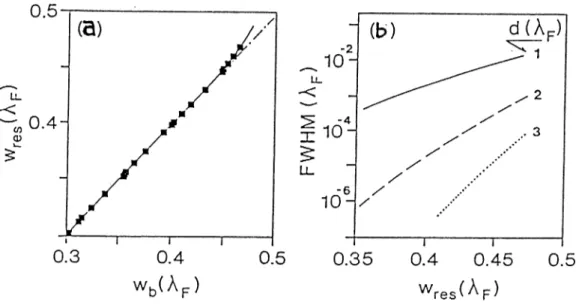
F ig u re 1.1: “Pros and cons” of miniaturization

(a) Number of atoms required to store one bit of information on a memory device. The straight line is a fitted exponential. From Reference 1. (b) Conductance of small ohmic contacts on GaAs as a function of contact size. The squares denote the average values obtained for macroscopically identical contacts. The full and dashed lines denote the extreme and average conductances, respectively. From Reference 2.

which becomes important when quantum mechanical and nonaveraging aspects of the system becomes dominant. This is only a single representative example for the complications of small systems from the point of view of technological and physical considerations. This study is devoted to the latter.

One of the most important features of the small systems is their sample specific properties. Our everyday experience conjectures that macroscopically identical systems have to yield the same results under identical experimental

(19)

conditions. However, for small systems this rule breaks down. As mentioned above, ohmic contacts fabricated on the same wafer using the same chemical and physical modification steps may have widely spread resistance values. Thinking in detail, this is very natural, however. It is known that the metal-semiconductor contact is not ordered and is made of grains. For a large contact, there is a large number of grains and the measured resistance is essentially an average of resistance of these grains. On the other hand, a small contact has only a small number of grains and this averaging can not be complete. Thus, the size and distribution of the grains may differ appreciably from one contact to other leading to the spread of resistance. Note that, this novel behavior is not solely due to the limited fabrication capabilities. Unless arranging the atoms one by one in a device, such effects will result independent of the technology used, due to the statistical nature of this arrangement. Taking a simpler example, for a macroscopic conductor contains a huge number of impurities and the resistance of the sample is determined according to Ohm’s law or microscopically according to the Einstein or Drude formulae. For a small sample, however, there are only a few impurities and their strengths and positions determine the resistance. The averaging for such a small system is not sufficient to result in the diffusion relation of Einstein or the resistivity relation of Drude.

Another important aspect of small systems is the geometry-specific properties. Miniaturizing the devices further one reaches to a limit for which the device does not contain any impurities at all. For this case, the quantum mechanical propagation along the sample is essential. The material properties, however, are suppressed to a large extent. That is, the same results may be obtained by using completely different systems of the same geometry. This very effect is present for the case described in the preceding paragraph, as well. Although the material properties determine the mean behavior, the variation around this mean value is independent of the material and either universal or specific to the geometry. This is, in fact, is the manifestation of the nonlocal nature of transport in small systems. For instance, adding or removing a new geometrical feature to the circuit away from the classical path of the flow of the current the measured quantities

(20)

are changed.

At this point we wish to replace the term small systems with the term “mesoscopic devices” hereafter (as derived from the Greek prefix meso=middle). The term mesoscopics corresponds to a length scale for which the averaging properties of the macroscopic world does not take place and the reversible and perfect mechanics of microscopic objects is not applicable. In what follows in this chapter we summarize the theoretical and experimental work has been done in the mesoscopic physics. The review is intended to be representative, but not exhaustive due to the limitation of space. More detailed information can be obtained from the recent conference proceedings on the subject.^"®

Chapter 1. Introduction to Mesoscopics 4

Ah a r o n o v- Bo h m Ef f e c t

One of the most important manifestations of the effects listed above came out of the studies on Aharonov-Bohm effect in solid state devices. Aharonov-Bohm effect, or more precisely the gedanken experiment of Aharonov and Bohm,^’® is one of the most important demonstrations of the importance of the phase of quantum mechanical wave function. If a flow of current is divided into two branches as shown in Figure 1.2 and these branches enclose a region of nonzero magnetic field, the electron wave function will have differing phases depending on the branch it follows. Therefore, two components of current will interfere at the output leading to the so called Aharonov-Bohm oscillations. The phase difference between the electron wave functions going from the upper and lower branches is

A(f> = ^ d\ · A , (1.1)

A being the vector potential. This phase yields to oscillations in conductance of the circuit since the wave function squared at the exit is given by

l^p ^ ^ V’2exp(zA<^)p, (1.2)

•01 and 02 being the wave functions corresponding to propagations through the

upper and lower branches, respectively, for zero-field. Consequently, conductance (or resistance) exhibits oscillations periodic in the magnetic flux enclosed by the

(21)

B C G a a s s )

F ig u re 1.2: Aharonov-Bohm effect for a metallic loop

Change in the resistance of a lithium film evaporated onto a quartz fiber of diameter 1.3 pm and length 1cm. The magnetic field is parallel to the fiber. Temperature is 1.5 °K and the resistance at zero magnetic field is 2 Kil. From Reference 9. The inset shows the schematics of the Aharonov-Bohm effect.

loop with period = h / e, the quantum of magnetic flux. The first experiments

using solid state devices carried out by Sharvin and Sharvin^ and Al’tshuler and coworkers^° and yield the results shown in Figure 1.2. It took a few years until the western experimentalists reproduce these results. The magnetoconductance curve shown in Figure 1.2 contains a number of very important features as long as mesoscopics is concerned.

Strikingly, the period of oscillations is #o/2, and not as expected.

This point was clarified by Al’tshuler and c o w o r k e r s . A c c o r d i n g to their explanation, the $<,/2 oscillations arise due to the interference of electrons enclosing the cylinder once clockwise and counterclockwise. Then the phcise difference is twice of that given in Equation 1.1 and thus, the period halves. Along the loop electrons may be scattered by some impurities, yet scattering along the

(22)

Chapter 1. Introduction to Mesoscopics 5. O 100 200 300 FREQUENCY [I/aH] 400

F ig u re 1.3: Aharonov-Bohm effect for a metallic ring

(a) Change in the resistance of a polycrystaline gold ring. The ring has inner diameter 0.8 pm, width 0.04 pm and thickness 0.04 pm. (b) The Fourier transform of the same data. From Reference 12.

two paths contribute exactly the same phase since they are time reversed forms of each other. On the other hand, the phase difference due to the scattering along the loop is different for electrons traversing only half of the circumference. Therefore,

the $0 oscillations are phase averaged due to the randomly varying phase along

the axis of cylinder. Using rings instead of cylinders it has become possible^^’^^ to observe $<, oscillations together with $<>/2 oscillations as shown in Figure 1.3. The phase averaging effect was also observed for N rings connected in series^^*

for which the $o/2 oscillations remain constant in amplitude and oscillations

decay as due to the random phase of oscillations for each ring. Another

important observation®’^® in Figure 1.2 is the decay of the oscillation amplitude with increasing magnetic field. This is caused by the finite thickness of the cylinder, thus different trajectories contribute different Aharonov-Bohm periods which are out of phase.

(23)

The most important observation from a mesoscopics point of view is the diminishing oscillation amplitude with increasing temperature. This point, again, was explained by Al’tshuler and coworkers^®’^^ using phase coherence arguments. Clearly, in a solid an electron suifers different kind of scattering processes. Some of these scattering events causes the electron to loose its phase. That is, knowing the phase of the electron wave function prior to the scattering one can not determine its phase after the scattering. This incoherence prevents the electron from displaying interference effects. It is possible, at least in principle,

to define a phase coherence length as the distance over which the electron

wave function retains its phase. If the circumference of the loop exceeds L^, then clearly the oscillations gets weaker. Al’tshuler and coworkers^^ showed that

this decrease is exponential, A.Rab cx exp (—C /L ^), C being the circumference.

In turn, decreases with increasing temperature due to the increased rate of

inelastic scattering. This way, we have a criterion for the mesoscopic nature of

any device. The related length scales are the phase coherence length the

electron mean free path £e, which is equal to the distance along which an electron moves without suffering any scattering, the Fermi wavelength Xp, and finally the size of the device L. It is common to use the elastic scattering length instead of £c and the inelastic scattering length instead of L^. However, these substitutions may not be correct in general and one has to be careful when using them. For

macroscopic devices one has Xp, L and therefore interference effects

are not observable. For mesoscopic device L < L ^ and the interference effects are nor averaged out. The mesoscopic devices may have both Xp, ¿e < L and Xp 7Ü L < le. They are called to be in the diffusive^ and ballistic regimes, respectively. For the second class there are no impurities in the devices so that the geometry specific features are pronounced.

The last observation from Figure 1.2 is the negative overall magnetoresistance. This again is related to the interference of the states enclosing the flux once in opposite directions. This corresponds to a constructive interference for scattering

^The term diffusive has to be differentiated from the usual diffusive transport, for which < L. This regime is also referred as elastic diffusive regime.

(24)

from + k state to the —k state/® that is to a coherent backscattering. This yields a larger amplitude for —k state than would be expected and thus to a larger resistance for zero magnetic field. For a finite magnetic field, however, different loops contribute different periods and thus a phase averaging leads to the negative magnetoresistance. This point may be helpful to study the phase

coherence length since as increases the effect of coherent backscattering gets

stronger. For further interest on the solid-state Aharonov-Bohm effect we refer to existing review papers on the subject.

La n d a u e r Fo r m u l a e

To this point the theoretical approaches to transport in mesoscopic devices have not been mentioned. Nevertheless, a complete understanding the mesoscopic physics requires a theoretical tool that can be used to find the conductance of a small sample for given arbitrary measurement conditions. For large samples phenomenological relations or approximations provide this tool. However, as described above for smaller samples these relations become irrelevant and a fully quantum mechanical theory which takes care of the position and strength of scatterers explicitly is required. Such approaches have been utilized since late 1950s. Kubo^® and Greenwood^® argued that the current through the sample is a cumulation of the local linear response of the system to an electromagnetic field. This electromagnetic field, in turn, is the external field plus the self-consistent field generated in response to it. The central entity in the Kubo formalism is the local conductivity tensor aap and the local current density ja is found by using

ia (r) = j dr aao{v,r)Ef3{T), (1.3)

where Ep is the local electric field and

o r,

/3 represent the cartesian components. In

a transport measurement the local electric field may not be known due to the fact that the system is not homogeneous. Therefore, first the electric field E{r) due to an applied bias has to be found, followed by the calculation of current density and the total current passing through the device. Although the Kubo formalism is proved to be appropriate for studying infinite systems, for mesoscopics it has

(25)

Chapter 1. Introduction to Mesoscoplcs

certain complications. In this regime it becomes necessary to calculate (Tap for each individual device. In addition to that, in the mesoscopic regime not the local quantities as cr(r, r^) but the global quantities as conductance describe the device. Nevertheless, it was shown that linear response theory may be used in mesoscopics by taking proper cautions. The generalized Kubo formalism as developed by Strëda and coworkers^®’^^ is even more appealing to some theorists than the scattering approach described below.

In the same year as Kubo published his results, Landauer^^ used an alternative line of thought to derive an alternative approach to quantum transport. His motivation was the reciprocity principle of the electrical circuit theory. According to this principle, both the voltage across or the current through the circuit may be taken as the external driving agent. Then the response of the circuit is the current or voltage, respectively. Landauer argued that instead of applying an external electric field as it is done in Kubo formulation, one equally may draw a current through the device and gets exactly the same result for the conductance. This approach has the advantage over the standard Kubo formula that it is possible to include the boundary conditions easily and global quantities can be found without too much problem. Landauer’s work and the following studies are widely referred as the scattering approach since they rely on the scattering of the incoming flux by the impurities in the sample.

The derivation of Landauer’s formula for conductance for a strictly one dimensional (ID) system is studied below in order to understand the underlying physics. Consider the system shown in Figure 1.4. The reservoirs on the left and right are assumed to satisfy the blackbody boundary conditions. That is, the incoming flux is totally absorbed and the outgoing flux is determined by the corresponding distribution function, for the case at hand by the Fermi-Dirac distribution. To this end, we assume that the left- and right-hand side reservoirs inject carriers into the sample up to Fermi levels pi, and pn, respectively. The current injected by the left electrode is in excess of that injected by the right one. Ignoring the scatterer for the time being, the total current passing through the sample is simply the flux of electrons traversing the sample per unit time. This

(26)

F ig u re 1.4: Calculation of conductance for a single scatterer

is equal to the product of the density of electrons and their velocity. The density, in turn, is the product of the density of states and the energy interval in which the left- and right-going electrons are unbalanced.

1 = evV{E)(^L — (1.4)

where v is the velocity of electrons with energy E . The density of states is given by the usual expression

where h^k'^/2m = E. Note that, the product vT>(E) is equal to l/irh and is independent of energy. Using this relation the current is found as

I = y (/ii - m ) · ( 1.6)

In the presence of the scatterer only a portion of this current can peiss through it and the rest is reflected back. Assuming th at the transmission probability is T, the current becomes

(1.7)

The difference of the Fermi energies, — p r), is chosen to be small so that

(27)

difference across the scatterer, on the other hand, can be found by calculating the effect of the charge piled up near the scatterer. This can be done using either self-consistent screening^^ or the Einstein r e l a t i o n . T h e electrochemical potential measured at the two sides of the scatterer can be found by employing a counting argument. The carrier densities on the left- and right-hand side of the

scatterer are represented by and //2, respectively. They can be determined by

equating the number of occupied states above p, to the number of unoccupied states below /z,· for z = 1, 2. Noting that the total number of states between pR

and PL is equal to 2V{E)(pl — Pr) and the density of electrons to the right and

left of the scatterer are TT>{E) and (1 -f- K)T>{E), respectively, one finds T {pL - P2) = (2 - T) (^2 - Pr),

(1 + R) {pL - pi) = ( 1 - R ) (pi - Pr),

(1.8)

(1.9) R — 1 —T being the reflection probability of the scatterer. The voltage difference

eV = Pi - p2.

can be easily found to yield

P i - P 2 = r{pL - Pr).

( 1.10)

(1.11)

(1.12)

Finally, the conductance G — I j V which is given by

^ h R ‘

Later Biittiker and coworkers^^ derived the multi-subband form of Equation 1.12 to find 9^2 _ 2 T Of,2 G = ^ - ^ E T . · . - 1 m

where u„, T„ and are the velocity, total transmission and total reflection

probabilities in the nth subband, respectively. The total transmission probability is obtained by adding the probabilities of transmission to the nth subband from

(28)

can be calculated by using the scattering matrix. Note that, the continuity of

current for the multi-subband case requires — T„).

The conductance formula Equation 1.12 had been rederived by several groups^®"^® by using various approaches. Anderson and coworkers^® used this formula and a multi-subband generalization to study the scaling theory of localization. Engquist and Anderson^® introduced the voltage probes in the system and found Equation 1.12 for weakly coupled voltage probes. Langreth and Abrahams^^ derived Equation 1.12 and its multi-subband generalization starting from the Kubo formalism. AzbeP® was the first who derived Equation 1.13 using scattering states.

Synchronously studies giving different results for the conductance were appeared in the literature, as well. For example, Economou and Soukoulis^® calculated the conductance for the strictly ID case shown in Figure 1.4 using Kubo formalism and found

2e2

G = ^ T, (1.14)

as compared to Equation 1.12. Later, Fisher and Lee®° employed the linear response theory for the multi-subband case and found that the conductance is given by

(1.15) 9^2

G = - ^ T r{ tt'} ,

t being the matrix of transmission probability amplitudes. The two sets of conductance formulae are approximately equal for the case i? ~ 1, that is, the opaque barrier limit. However, for the other extreme i? ~ 0, that is, for the transparent barrier limit Equations 1.12 and 1.13 yields infinite conductance, compared to the finite value obtained from Equations 1.14 and 1.15. These four formulae are usually referred as Landauer formulae. The first two are differentiated from the last two by classifying them as G ~ T / ( l — T) and G ^ T formulae, respectively. It is striking that different groups obtained different answers by using Kubo formalism. This difference is, in fact, due to the different assumptions made about the measured quantities, self-consistency etc.

(29)

The problem about the G T formula was that for a perfect conductor it gives

a finite conductance 2e^N/h, N being the number of occupied subbands. This contrasts the intuitive expectation that the perfect conductor has no resistance. On the other hand, the G ~ T / ( 1 —T) formula gives infinite conductance and thus zero resistance for a perfect conductor. Imry®^ showed that the resistance given by the G ~ T is a contact resistance and does not corresponds to the sample at hand, i.e, the perfect conductor. Using two containers of Fermions with different densities, and attached to each other by a narrow tube he found that the current through the tube is / = a{2e^N jh){pi, — pn), a being a constant of the order of unity. In this example, the tube has no scattering center in it and perfectly matched to the containers so that it can be thought as a perfect conductor, and it still yields a finite conductance. This conductance is, in fact, associated with the contacts between the containers and the tube and is similar to the classical contact resistance. One may, at this point, think that for a classical transport measurement the effect of the contact resistances may be eliminated by using a four-probe geometry. That is, by using different probes for the current and voltage measurements. The resistance of a perfect conductor vanishes only for this four-probe measurement. Consequently, it has been thought that the G ~ T formula applies for a two-probe measurement and G ~ T / ( l — T) for a four- probe measurement. This point had been taken for granted until the recent experimental results forced the theorists to think on the Landauer formulae once more as described below.

Un i v e r s a l Co n d u c t a n c e Fl u c t u a t i o n s

One of the most important problems arising from the results of the Aharonov- Bohm experiments carried out by rings^^’^^ was that, in addition to the and $o/2 periodic oscillations there were aperiodic fluctuations in resistance as a function of magnetic field as shown in Figure 1.3. These oscillations were reproducible for a single sample as long as it is not heated, but differ from sample to sample even though all the samples have the same macroscopical form. Thus, these oscillations were taken to be the magnetofingerprint of the

(30)

specific sample at hand. The period of these oscillations is larger than $o and in the power spectrum as a function of frequency these oscillations appear as an increase near zero frequency. Strangely enough, same kind of oscillation were found for completely different mesoscopic devices, such as wires,^^ Si inversion layers^® (conductance fluctuations as a function of the gate voltage) and for an Anderson modeP^ (theoretical calculation of conductance). These systems have average conductances varying by orders of magnitude while the amplitude of the

fluctuations is approximately constant and of the order of ~ (e^/h) I f (25800 0)

irrespective of the average conductance. Therefore, these fluctuations are often referred as the universal conductance fluctuation^.

The theoretical understanding of the universal conductance fluctuations followed the work done on weak localization. Up to this point we mentioned “disordered” systems or “metals” without explicitly defining these terms. It has long been recognized that for disordered systems some of the electronic states are localized and the transmission coefficient is exponentially small in the device size.^® This situation is in contrast with the transport theories we discussed in the preceding subsection, since if the states near the Fermi level are localized it is not possible to talk about propagating electrons. Fortunately, the localization comes into the picture with a relevant length scale as the other physical effects do. This length is called the localization length ^ and the resistance of the sample increases as ~ exp (L f^) for ^ < L. This is generally referred as the strong localization regime. In this regime the transport occurs via Mott hopping or resonant tunneling. Thus, the density of states has spikes with large peak value but exponentially small resonance w i d t h . C o n s e q u e n t l y the conductance has large fluctuations as a function of the Fermi level or impurity configuration. For strong localization regime the resistance is both non-Ohmic and have fluctuations which do not average out. These fluctuations are clearly not “universal” in the sense defined above.

Now consider the case for which L < C Clearly the exponential decay * *The “universality” of these fluctuations were discussed and defined with its limitations in the literature to which we refer in this subsection.

(31)

of the localized wave functions does not dominate the transport properties, rather the Bloch states are scattered by the disorder. Therefore, it is possible to use the Kubo or Landauer formalisms for quantum transport. This case is referred as the weak localization regime of metallic conduction. The early theoretical understanding on weak localization can be found in the related review p a p e r s . I t is possible to investigate the weakly localized sample in terms of the resonant tunneling transport as it is done for strong localization. For this case, however, the resonances are overlapping leading to a rather smooth density of states. Thus, it is possible to have fluctuations which are independent of the size of the system and the strength of disorder. In fact, within the weak localization theory it is shown that the density of states have important statistical aspects^®’^^ which contribute to the conductance fluctuations.

Returning back to the universal conductance fluctuations, one observes that the transport in such weakly localized samples can be described by a random-walk type elastic diffusion. Therefore, one has a large number of randomly intersecting electron trajectories which interfere with each other as given by

i ~ y ) exp (i(^, - <A,)

1

,

(

1

.

16

)

r and s denoting two different paths connecting the same end points and <j)r and (f>s are the respective phases attained going through these paths. Since this interference is not averaged out in mesoscopics and contributes to the conductance of the sample. Any perturbation that changes these phases causes fluctuation of the transmission probability, and thus of the conductance. Such a perturbation may be obtained by several means such as by changing the impurity configuration, by applying a magnetic field and thus adding an Aharonov- Bohm phase to the zero-field pheise difference, and by varying the Fermi level. Although this qualitative explanation agrees with the experimental observations, the universality of the fluctuations can not be extracted therefrom.

The breakthrough for the quantitative understanding of the universal

conductance fluctuations was the ergodic hypothesis.“^^’“^^ According to this

(32)

a sufficiently large magnetic field or energy range would be equal to the corresponding average taken for an ensemble of macroscopically equivalent

systems. Therefore it suffices to consider the statistical properties of the

conductance for an ensemble of impurity configurations. For example, the

variance of these fluctuations is given by < >» < · · · > denoting the ensemble

averaging and AG^ = G^— < >. This value was shown to be of the order

of (e^//i), independent of the average conductance of the system.^®""*^ The exact number, however, depends on several details of the system and is not “universal”. Another important quantity is the conductance correlation function F{6B^6E) defined as

F{SB, SE) =< A G {B , E )A G {B + 6 B , E + BE) >, (1.17)

which determines the spacing of the fluctuations in magnetic field and Fermi energy. It was shown^°~^^ that F{6B, SE) is a decreasing function of its arguments with the corresponding half-widths Be and Ec, respectively. The natural scale of magnetic field Be is of the order of $o/-A, A being the area of the largest loop through which the phase coherence is retained. This is exactly the necessary magnetic field variation in order to change the phase difference of the interfering

wave functions by 27t. The energy scale Ee, on the other hand, is of the order

of the energy spread due to the inelastic scattering in the sample. < A G “^ >, Be and Ec can be calculated exactly as given by Lee and c o w o r k e r s . A systematic analysis of universal conductance fluctuations in Si inversion l ayer s s howed that the agreement between the experiment and theory is excellent.

Mu l t i p r o b e Me a s u r e m e n t s

The controversy on the Landauer formulae had been perceived as an academic

problem until universal conductance fluctuations were observed. This was

due to the fact that for most of the systems under consideration i? ~ 0 so that G ~ r and G ~ T /( l — T) formulae give approximately the same

answer. However, the universal conductance fluctuation experiments result

an unexpected asymmetry in conductance.^^ This observation later supported by the magnetic field asymmetry of magnetoconductance of loops and wires'*®

(33)

and voltage fluctuations^®’'*^ measured for multi-probe devices. Clearly, the

G ^ T type Landauer formulae yields G{B) = G{—B) and are not consistent with the experiments. The multi-subband generalization oi G ^ T/{1 — T) type formulae as given in Equation 1.13, on the other hand, does not have such a symmetry. This asymmetry, however, is not sufficient to explain the experimentally observed asymmetry in universal conductance fluctuations.®^ Thus, the question concerning the relevant Landauer formula had become a serious confrontation with experimental results.

The symmetry of electrical conduction is a well known aspect of electro

magnetic theory. The local conductivity tensor <7^/3 satisfy the Onsager-Casimir

symmetry relations^®

a,p(B) = a p , { - B ) . (1.18)

In addition, the reciprocity relation for multi-probe measurements were known since the first decade of the century in the absence magnetic field. It relies on the reciprocity of the current and voltage sources so that

Bfnn,kl — (1.19)

Here the multi-probe resistance R m n , k i is defined as the ratio of the voltage

difference measured between the probes k and / to the current injected from probe m and drawn out of probe n

V k - V i

Rmn^kl

(

1

.

20

)

The generalization of the reciprocity relation to finite magnetic fields is more recent^** and gives

Rm n , k l { B) = Rkl,mn{ — B ) . (1-21)

Although the presence of local symmetry as given by Equation 1.18 leads to the reciprocity relation, the reverse is not true. That is, it is possible to have a nonsymmetric local conductivity tensor and the global symmetry in Equation 1.21 is preserved.

Biittiker®®’®* argued that the discrepancy between the Landauer formulae and the experimental results arises from the handling of the voltage probes. In

(34)

deriving Equations 1.12 and 1.13 the voltage probes were taken to be weakly coupled to the device. This point earlier mentioned in the derivation of Engquist and Anderson.^® On the other hand, Equations 1.14 and 1.15 correspond to a two-probe measurement. In the experiments, however, the lithographic shape of the current and voltage probes are the same. Thus, it is not possible to think about the weak coupling of the voltage probes. Biittiker considered the coherent device consisting of the probes in addition to the loop or wire, and calculated the scattering matrix for this device. All the probes are assumed to be connected to reservoirs in equilibrium. The current going into the device through probe m is found to be

Im — ^ j 9mn(f^m /^n)> (i.22)

m

where gmn is the generalized conductance for probes m and n, and is given by

9ran — ^ (1.23)

T representing the matrix ( tv ). The electrochemical potentials of the

probes [pn] are calculated by considering the current through the macroscopic connections of the probes. For example, in order to calculate Rmn.ki one takes Im — —In = I and li = 0 for all the other probes. Inverting the matrix equation

Equation 1.22, one gets all the electrochemical potential differences and thus,

(Yk — Vi) = {pk — Pi)/^· The four terminal resistance is Rmn.ki = y / I - Note that, this multiprobe Landauer formula is a natural extension of the original Landauer formulae, as far as the external excitation and scattering matrix are concerned. Buttiker®°’®^ showed also that the four-probe resistance calculated

from Equation 1.22 and 1.23 satisfies the global reciprocity relation Equation 1.2 1.

The asymmetry of the magnetoconductance curves'^® was shown to be exact agreement with the predictions of this multi-probe Landauer formula.

It is interesting to study the limits of Equation 1.22 and 1.23. For the two- terminal resistance it reduces to Equations 1.14 and 1.15 as expected. For four- probes, voltage probes being weakly coupled, the G ~ T /( l — T) formula is obtained for the single-subband case. For multi-subband systems the expression is complicated and does not simplify any conventional Landauer formula. The

(35)

multi-channel generalizations of G ~ T / i l — T) are irrelevant due to the incomplete treatment of the voltage probes. It is also possible to obtain negative four-probe conductance as shown by Büttiker®^ for some systems. This is not contradicting any physical principle, since the power disspated in the circuit is proportional to the conductance found by using G ^ T formula and is always positive. This formalism was also used to investigate the voltage fluctuations®^"®® due to the nonlocal nature of mesoscopic transport and had considerable success.

Finally, we wish to mention important contribution by Stone and cowork-

gj,gS6,57 a]jout the equivalence of the Kubo and Landauer-Biittiker formalisms.

Starting from the standard linear-response theory and explicitly including the probes in their formalism they showed that the Kubo formulation yields Landauer-Biittiker relations both in the absence®® and in the presence®^ of magnetic field. These derivations together with the success of Landauer-Biittiker approach seemingly ceased the controversy on the Landauer formula. We focus our attention on this discussion once more in the last section of this chapter.

1 .2

Q u a n tu m P o in t C o n ta c ts

One of the most important breakthroughs in mesoscopic physics is the observation of the quantization of conductance in quantum point contacts (QPC).®®’®® Earlier different methods used to obtain mesoscopic devices in the diffusive regime as

exemplified in Section 1.1. Note that, however, in the diffusive regime the

quantum size effects are not essential due to relatively large device size and presence of scatterers. In the other regime of mesoscopics, namely for ballistic transport, the electrons traverse the device without suffering any scattering. Consequently, the size effects and geometry-specific features are the determining factors for ballistic devices. The fabrication of the ballistic devices was hindered

due to the technological constraints until recently. In order to satisfy the

requirements of ballistic transport the size of the device L has to be smaller than the electron mean free path 4 and comparable to the Fermi wavelength A^. The first requirement guarantees that scattering in the device to be prohibited.

(36)

Chapter 1. Introduction to Mesoscopics 20 e l e c t r o d e A I G a A s 2 D E G G a A s DEPLETED REGION

F ig u re 1.5: Schematic layout of a quantum point contact (a) Cross-sectional and (b) top views of a quantum point contact

It can be achieved by using highly pure samples. The latter one, on the other hand, is the condition for the quantum size effects to come into the play. One way of achieving this is to decrease the electron density and thus to increase Xp. However, for low density 2D electron gas (EG) the screening is weak and localization takes place. That is, it is necessary to miniaturize the device without decreasing the density. Therefore, the fabrication of QPC became a possibility only after the growth of high-mobility samples and advents in ion- and electron- beam lithography.

In Figure 1.5 the schematic layout of a QPC is shown. The 2D EG is

obtained by a modulation doping AlGaAs/GaAs heterojunction and ought to have a mobility on the order of 10® cm^-V“^-sec“^ and the Fermi wavelength is a few hundred angstroms. On top of the sample a split-gate is defined by ion- or electron-beam lithography. The gap between the gates has to be comparable with Xp· and the width of the gate has to be smaller than 4 · That is, both the width

(37)

Chapter 1. Introduction to Mesoscopics 21 UJ U 2 < b D C Z o u

F i g u r e 1.6: Q uan tizatio n of conductance of a q u an tu m point contact The two-probe conductance of a quantum point contact as a function of the gate voltage. The tem perature is 0.6 °K and the conductance is obtained using the data for resistance measurement after subtraction of background resistance of 400 fl. From Reference 58.

and gap has to be a few hundred angstroms. The measurements are carried out

via probes attached to the 2D EG by ohmic contacts and a negative gate voltage

Vg is applied between the split-gate and substrate. For slightly negative gate voltages, the effect of the split-gate is small and the measurements yield results

characteristic to 2D EG. For more negative gate voltages the electrons beneath the

split-gate are depleted and a channel is obtained in the 2D EG. The characteristics

of this novel device is quite different than that of a 2D EG since the electrons are

constricted to flow from this channel. Increasing the negative gate voltage, the channel gets narrower due to stronger depletion. That is, it is possible to vary the width of the QPC externally for a given device configuration only by changing

Vg. Further increasing the negative gate voltage all the electrons underneath the

gate region are depleted, leading to the complete pinching off of the device. The easiest measurement that can be carried out by such a QPC is the measurement of the two-terminal resistance. The Delft-Philips collaboration®^ and Cambridge

(38)

group®^ succeeded to perform this measurement in late 1987. Their results were striking and the conductance (or resistance) of the QPC is found to change in steps for continuously varying Vg as shown in Figure 1.6.

In fact, the concept of point contacts was familiar to condensed m atter physics for a w h i l e , t h o u g h , in a different context. The point contacts had been used to study the Fermi surfaces®® and phonon scattering®^ in metals. The difference between the QPC and the earlier point contacts was the ratio of the device size to the Fermi wavelength, LfXp· As a result, only for the QPC quantum size effects are possible to play an essential role. For the earlier point contacts this ratio weis of the order of hundred, compared to unity for QPC. Methods of clcissical electrodynamics and kinetic theory of gasses were used to analyze the conductance of point contacts. First Sharvin®® incorporating the Fermion nature of electrons and using the Drude approximation for resistivity conjectured that the conductance of a point contact is independent of material parameters and is determined solely by the electron density and geometry. For a 2D point contact of width w, the Sharvin conductance is given by

^ 2e2 2w

= X i;*

(1.24)

including spin degeneracy. Although the experimental results shown in Figure 1.6

are in qualitative agreement with the trend G ~ w/ \f, the staircase structure is

not consistent with the continuous change of Gs as a function of width w. The striking feature in the experimental results is that the change in the conductance between consecutive plateaus (where the conductance G is approximately stays

constant with changing Vg) is equal to 2e^//i within a precision of few percent.

This magic number is the prefactor in Equation 1.24 and is called the quantum of conductance.

The quantum of conductance 2e^//i was one of the central entities in

mesoscopic physics as shown in Section 1.1. As early as 1957, Landauer^^’^®

pointed out the essential connection between electronic transport and this magic number as described above. Later, Imry®^ showed that for a perfectly conducting narrow connection between two wide electron reservoirs the conductance is

(39)

of the order of this magic number. However, the observed quantization of

the conductance in QPC had not been anticipated by theorists prior to the experiments. The reason of this can even be sought in the experimental results. To date, the precision of quantization in QPC is one percent, part of which may

be thought as an intrinsic deviation from quantization^ On the other hand, ¡h

can be measured by use of quantum Hall effect®^ within an accuracy of one part

in 10^. That is, the quantization of conductance in a QPC is not exact and,

in fact, highly distorted. Before the pioneering experiments®®’®^ this distortion was expected to wash out the main effect, namely quantization. Actually, dirty electron waveguides, which does not yield quantization, were used to understand the diffusive regime of mesoscopics as depicted in the preceding section. Only after the experiments it became clear th at the quantization may be robust against several interfering effects.

We have to admit that the development of the nanotechnology took over the theoretical studies and experiments leaded the theorists in the subject of QPC at the early stages. Nowadays, the QPC is used to analyze several important aspects of electronic properties and transport in condensed systems. Especially, magnetotransport measurements carried out by use of QPC provide unique opportunities to investigate the behavior of mesoscopic systems with applied magnetic field. These subjects, however, are beyond the scope of this study. To our knowledge a wide review of the studies of the Delft-Philips collaboration constitutes the best reference for the experimental work that have been done in the field.®® On the other hand, several groups shed light on the theoretical

basis of the quantization of conductance as described in Section 2.1. The current

focus of interest from theoretical point of view is the reexamination of Landauer formulae and electronic transport in mesoscopic systems by considering QPC and electron waveguides as the main building blocks.

The existing theoretical tools at the time of the experiments were sufficient to explain the quantization in simple terms.®®’®^ The subband formation was well

understood and exploited earlier.®'* Clearly, the accumulation layer of the 2D EG