Designing, fabrication and post- fabrication characterization of half-frequency driven 16 x 16 waterborne transmit CMUT array

(1)

DESIGNING, FABRICATION AND

POST-FABRICATION CHARACTERIZATION OF

HALF-FREQUENCY DRIVEN 16 X 16

WATERBORNE TRANSMIT CMUT ARRAY

A THESIS SUBMITTED TO

THE GRADUATE SCHOOL OF ENGINEERING AND SCIENCE

OF BILKENT UNIVERSITY

IN PARTIAL FULFILLMENT OF THE REQUIREMENTS FOR

THE DEGREE OF

MASTER OF SCIENCE

IN

ELECTRICAL AND ELECTRONICS ENGINEERING

By

Yusuph Abubakar Abhoo

February 2021

(2)

Designing, Fabrication and Post-fabrication Characterization

of Half-frequency driven 16 x 16 Waterborne Transmit CMUT Array By Yusuph Abubakar Abhoo

February 2021

We certify that we have read this thesis and that in our opinion it is fully adequate, in scope and in quality, as a thesis for the degree of Master of Science.

Hayrettin Köymen (Advisor)

Abdullah Atalar

Itır Köymen

Approved for the Graduate School of Engineering and Science:

Ezhan Karaşan

Director of the Graduate School

(3)

ABSTRACT

DESIGNING, FABRICATION AND POST-FABRICATION

CHARACTERIZATION OF HALF-FREQUENCY DRIVEN

16 X 16 WATERBORNE TRANSMIT CMUT ARRAY

Yusuph Abubakar Abhoo

M.S. in Electrical and Electronics Engineering Advisor: Hayrettin Köymen

February 2021

Capacitive Micromachined Ultrasonic Transducers (CMUT) are micro-scaled electromechanical devices which are used to either transmit or receive pressure signals and applicable for various purposes such as ultrasonic sensor, medical imaging, accurate biometric sensing and parametric speakers. For transmitting CMUT transducer, different sizes and array configurations are used to intensify the transmission power depending on the application. The half-frequency driven waterborne transmitting CMUT array designed in this work is to be used for high resolution volumetric medical imaging purpose. This was accomplished by a design which prioritizes maximizing the power output, achieving a directive radiation pattern with low sidelobes which maximizes the beamformable region. In this work, the issues with steering of the focused beam are also resolved to achieve a focused steerable beam. This work is an advancement from the earlier designed half-frequency driven airborne transmit CMUT to improve power output, introduce the beamforming and focused transmission capabilities and be applicable for high resolution volumetric medical imaging purpose.

To improve the power output, the design was made to compensate for the static depression. Compensating for static depression was achieved by designing to operate the CMUT without DC bias voltage which allows for full-gap swing and giving output signal of twice the input frequency. This property allows the cell to produce high power output with low voltage levels but also brings the advantage of operating the cell with very high voltages without collapsing.

(4)

The CMUT was chosen to be operating at 7.5 MHz and be driven by Digital Phased Array System (DiPhAS) which allowed to have maximum of 256 channels which for volumetric transmission meant a maximum of 16 x 16 array. Since the radiation pattern and Rayleigh distance are both the functions of radius, frequency and the pitch, the design optimization was found while considering all the above preferences simultaneously. The cells’ radii were determined to be 80 µm, the plate thickness was 15 µm, the gap height was found to be 117 nm and the pitch was 192 µm. The array designing was carried out using the large-signal equivalent circuit model and the radiation impedance matrix phenomenon.

The simulations showed that with this design, the maximized Rayleigh distance was 45.3 mm and the sidelobe of -17.4 dB. In simulations, very high pressure outputs were achievable with individual cells up to 425 kPa per cell with 150 VPP input while up to 1.5 MPa was emitted by the array plane wave transmission with only 10 VPP inputand almost doubles when the transmitted beam was focused at zero degrees. Fabrication was done by the wafer boding and flip-chip bonding techniques where the whole process required only two lithography masks.

After fabrication, the tests were performed to identify the yield of the transducer was 18.75% of the array then impedance analysis was done to characterize the functional cells and resonance frequency drift. The transducer was cased in a water-tight manner and the waterborne transmission were done with individual cells to characterize and compare the performance with the design simulations which were in the range of agreement achieving an average of 1625 Pa per cell. The functional cells were then used for plane wave transmission with 10 VPP and the output pressure of 397 kPa was achieved at resonance frequency. The measurement results showed that the design could further be improved by compensating the active area to improve the yield for better results and be able to use it for high resolution 3D medical imaging.

Keywords: CMUT, Array, Half Frequency Operation, Unbiased mode operation,

Radiation Impedance, Waterborne transmission, Volumetric Imaging technique, CMUT Lumped-element equivalent circuit, Microfabrication, MEMS

(5)

ÖZET

YARI FREKANSTA SÜRÜLEN SUALTI 16 X 16 ELEMANLI

CMUT DIZININ DIZAYNI, FABRIKASYONU VE

FABRIKASYON SONRASI KARAKTERIZASYONU

Yusuph Abubakar Abhoo

Elektrik ve Elektronik Mühendisliği, Yüksek Lisans Tez Danışmanı: Hayrettin Köymen

Şubat 2021

Kapasitif Mikro İşlenmiş Ultrasonik Dönüştürücüler (CMUT), basınç sinyallerini iletmek veya almak için kullanılan ve ultrasonik sensör, tıbbi görüntüleme, doğru biyometrik algılama, parametrik hoparlörler ve daha birçok alan gibi çeşitli amaçlara uygulanabilen mikro ölçekli elektromekanik cihazlardır. İletim CMUT dönüştürücüleri için, uygulamaya bağlı olarak iletim gücünü yoğunlaştırmak için farklı boyutlar ve dizi konfigürasyonları kullanılır. Bu çalışmada tasarlanan yarı frekansla çalışan su bazlı iletici CMUT dizisi, yüksek çözünürlüklü volümetrik tıbbi görüntüleme amacıyla kullanılacak. Bu, güç çıkışını en üst düzeye çıkarmaya öncelik veren, hüzme biçimlendirilebilir bölgeyi en üst düzeye çıkaran düşük yan çubuklarla yönlendirici bir radyasyon modeli elde eden bir tasarımla gerçekleştirildi. Bu çalışmada, odaklanmış yönlendirilebilir bir hüzme elde etmek için odaklanmış hüzmenin yönlendirilmesi ile ilgili sorunlar da çözülmüştür. Bu çalışma, güç çıkışını iyileştirmek, hüzmeleme ve odaklanmış iletim yeteneklerini tanıtmak ve yüksek çözünürlüklü volümetrik tıbbi görüntüleme amacına uygun olmak için daha önce tasarlanmış yarı frekans tahrikli havadan iletim CMUT'tan bir ilerlemedir.

Güç çıkışını iyileştirmek için, statik çöküntüyü telafi eden bir tasarım yapıldı. Statik çöküntüyü dengeleme, CMUT'u DC ön gerilim voltajı olmadan çalıştıracak şekilde tasarlayarak, tam aralık salınımına izin vererek ve giriş frekansının iki katı çıkış sinyali vererek sağlandı. Bu özellik, hücrenin düşük voltaj seviyelerinde yüksek güç çıkışı üretmesini sağlarken aynı zamanda hücreyi çökmeden çok yüksek voltajlarla çalıştırma avantajını da beraberinde getirir.

(6)

CMUT, 7.5 MHz'de çalışacak ve hacimsel aktarım için maksimum 16 x 16 dizi anlamına gelen maksimum 256 kanala izin veren DiPhAS tarafından çalıştırılacak şekilde seçildi. Işıma örüntüsü ve Rayleigh mesafesi hem yarıçap, frekans hem de aralık mesafesinin fonksiyonları olduğundan, tasarım optimizasyonu, yukarıdaki tüm tercihler aynı anda dikkate alınarak bulunmuştur. Hücrelerin yarıçapları 80 µm, plaka kalınlığı 15 µm, boşluk yüksekliği 117 nm ve aralık 192 µm olarak belirlendi. Dizi tasarımı, büyük sinyal eşdeğer devre modeli ve radyasyon empedans matrisi fenomeni kullanılarak gerçekleştirildi.

Simülasyonlar, bu tasarımla, maksimize edilen Rayleigh mesafesinin 45,3 mm ve yan lobun -17,4 dB olduğunu gösterdi. Simülasyonlarda, 150 VPP girişli hücre başına 425 kPa'ya kadar tekli hücrelerle çok yüksek basınç çıktıları elde edilebilirken, yalnızca 10 VPP girişli dizi düzlem dalga iletimi tarafından 1.5MPa’a kadar iletim yapıldığı ve iletilen hüzme 0 dereceye odaklandığında bu değerin 2 katına kadar çıktığı görülmüştür. Üretim, tüm işlemin sadece iki litografi maskesi gerektirdiği gofret kaplama ve flip-chip bağlama teknikleriyle yapıldı.

Üretimden sonra, dönüştürücünün veriminin, dizinin % 8.75'i olduğunu belirlemek için testler yapıldı, ardından fonksiyonel hücreleri ve rezonans frekans kaymasını karakterize etmek için empedans analizi yapıldı. Dönüştürücü, su geçirmez bir şekilde muhafaza edildi ve su bazlı iletim, hücre başına ortalama 1625 Pa'ya ulaşan mutabakat aralığındaki tasarım simülasyonları ile performansı karakterize etmek ve karşılaştırmak için ayrı hücrelerle yapıldı. Fonksiyonel hücreler daha sonra 10 VPP ile düzlem dalga iletimi için kullanıldı ve rezonans frekansında 397 kPa çıkış basıncı elde edildi. Ölçüm sonuçları, daha iyi sonuçlar için verimi iyileştirmek ve yüksek çözünürlüklü 3D tıbbi görüntüleme için kullanabilmek için aktif alanı telafi ederek tasarımın daha da geliştirilebileceğini gösterdi.

Anahtar Kelimeler: CMUT, CMUT dizi, Yarı frekansta operasyonu, Yüklemesiz

operasyon, radyasyon empedansı, Sualtı operasyon, hacimsel görüntüleme tekniği, Büyük ışaret eşdeger devre modeli, Mikrofabrikasyon, MEMS

(7)

Acknowledgements

Special thanks and highest appreciation to my advisor Prof. Dr. Hayrettin Köymen who made me into what I am today with his incredible technical and moral support throughout my master’s program at Bilkent University. Prof. Köymen has been more than just my mentor in the academic work, always had time to meet up for discussions, always gave his professional and friendly opinion a matter based on his vast experience and was always clear on what needs to be done. I have learnt a lot more than just the technical knowledge from him.

I would like to extend my sincere gratitude to Akif Sinan Taşdelen and Asst. Prof. Mehmet Yılmaz for their valuable time, technical mentoring and support they have given me throughout my thesis work with a lot of patience and care.

I would like to acknowledge and thank Prof. Dr. Abdullah Atalar for the knowledge I have gathered as member of our research group, instructor of one of my courses and for being part of the Jury for my defense.

This work would not have been completed without Kerem Enhoş who initiated this work to whom a lot of thanks and appreciation go. The support from my colleagues and other members of our research group was very significant and cannot go without acknowledging Asst. Prof. Itir Köymen, Dr. Fikret Yıldız, Giray İlhan, Murat Güngen, Abdulmalik Madigawa, Abdallah Alkilani, Yasin Kumru and Doğu Kaan Özyiğit.

Finally, I would like to deeply thank my wife, Ronak for being here with me away from home to give me the support I needed to keep going with the work. I would also like to thank my father, Abubakar and mother, Masad for always giving me wise words and advices whenever I needed them. I hope this work will be the beginning of more to come and positively affect all those close to me.

(8)

List of Figures

2.1 The cross-section of a depressed membrane CMUT with geometrical

illustration……….………..3

2.2 The equivalent circuit of transmit CMUT in large signal. ... 4

2.3 The CMUT array equivalent circuit with the impedance matrix, Z…..……….6

3.1 The location of the cells to be analyzed……….………...12

3.2 Simulation flow diagram……… . .13

3.3 Pressure output frequency response between 1 MHz – 20 MHz with 150 VPP and unbiased………..14

3.4 Particle velocity frequency domain analysis between 1 MHz – 20 MHz at 150 VPP…..……….15

3.5 Admittance values at 10 VPP………...16

3.6 Admittance values at 150 VPP………..17

3.7 Admittance response to change in input voltage at 7.5……….17

3.8 Transient analysis at 10 VPP and 3.75 MHz input signal………18

3.9 Transient analysis at 150 VPP and 3.75 MHz input………19

3.10 Normalized steady state membrane displacement at 7.5 MHz with 150 VPP input voltage at 3.75 MHz……….………19

3.11 The steady state normalized membrane displacement at 298.4 VPP and 3.75 MHz input signal……….20

3.12 The steady state output pressure from each CMUT cell excited at MVM, 298.4 VPP and at resonance frequency……….21

(11)

3.13 Particle velocity profile observed with one cycle signal of 300 VPP and 3.75

MHz ... 21

3.14 Transient response of 5-Cycle Gaussian-enveloped tone burst signal of 10

VPP at 3.75 MHz……….22

3.15 Transient response of 5-Cycle Gaussian-enveloped tone burst signal of 150

VPP at 3.75 MHz………23

3.16 Transient response of 5-Cycle Gaussian-enveloped tone burst signal of 372.3

VPP at 3.75 MHz………23

3.17 Normalized membrane displacement analyzed at 372.3 VPP of 5-cycle

Gaussian-enveloped tone burst signal……….…24

3.18 Particle velocity profile analysis at 372.3 VPP of 5-cycle Gaussian-enveloped

tone burst signal. Peak observed at 1.362 m/s………..24

3.19 The CMUT array as designed in the k-wave space……...………25

3.20 Simulation space created in k-wave with the transducer located at X=0 and

the sensor voxels as well as PML voxels placed radial to the transducer at 15.744 mm………26 3.21 Radiation Patterns formed in k-wave Vs. the computational radiation pattern

………..27

3.22 The beamforming at points of interest, 0o, 15o, 30o, and 60o from the normal

along with the plane wave transmission………..29

3.23 Power of Individual CMUTs analyzed from the corner, middle and side

Elements……….30

3.24Power radiated into the medium by the Transducer………30

4.1 The full CMUT transducer mask with wires and electrical pads………..…33

(12)

4.2 The Microscope images of the completely etched Epoxy wafer………...34

4.3 Image from Microscope after deposition of TiPtAu stack………...36

4.4 Before (left) and after (right) Alumina etching………..36

4.5 The microscope image of the CMUT cell right before wafer bonding……..37

4.6 The full wafer after modified bonding recipe (left) and damaged electrical

pads after wafer bonding (right)………..37

4.7 Metal deposition on the top membrane with the shadow mask (left) and the

wafer after complete removal of Silicon layer on electrical pads (right)…....38

4.8 Photoresist stripped, and the chrome etched……….39

4.9 A finalized single diced CMUT transducer chip………39

4.10 Flip-chip bonded Chip/PCB pair and ground pads connected……….40

4.11 Parylene C coated Chip/PCB pair on the transmitting side (left) and Epoxy

coated on the backside (right)………...41

4.12 Epoxy coated at the rim of the Chip/PCB bond at the transmitting side……..42

4.13 Mounting of the vertical PCBs socketing on the connectors………...43

4.14 Casing of the finalized transducer with connection coaxial cables…………. 43

5.1 Transducer array with labeled 48 functional cells; 26-Green colored cells from first group, 18-purple colored cells from second group and 4-red colored

cells from third group………...46

5.2 Impedance measurement setup with Impedance Analyzer and probestation...46

5.3 Admittance of the 255th cell excited at 1 VPP AC and 40 VDC bias in air……47

5.4 Admittance of the 227th cell excited at 1 VPP AC and 40 VDC bias in air...….47

5.5 Admittance of the 208th_{cell excited at 1 V}

PP AC and 40 VDC bias in air……48

(13)

5.6 The modified large signal equivalent circuit……….………50

5.7 The block diagram of the SR844 Lock-in Amplifier……...……...…………..53

5.8 The inside of the DSP of the SR844 Lock-in Amplifier………….…………..54

5.9 Visualized signal (left) and the X and Y values from the amplifier (right)…..54

5.10 Transducer array with labeled 48 functional cells; 26-Green colored cells

from first group and 22-purple colored cells from second group …...…55

5.11 The setup for transmission measurements with signal generator and reception

with hydrophone………56

5.12 The transducer array with functional connected cells colored in red………58

5.13 Pressure emitted by 48 functional cells of the transducer with a frequency

sweep from 1 MHz to 12 MHz………...59 A.1 Admittance for 15 Vac input with a frequency sweep 2.5 MHz – 20 MHz…68 A.2 Admittance for 35 Vac input with a frequency sweep 2.5 MHz – 20 MHz…68 A.3 Admittance for 55 Vac input with a frequency sweep 2.5 MHz – 20 MHz…69 A.4 Transient analysis with a continuous PWM signal of 10 VPP at 3.75 MHz…69 A.5 Transient analysis with a continuous PWM signal of 150 VPP at 3.75 MHz..70

A.6 Transient analysis with a continuous PWM signal of 262 VPP (MVM) at

3.75 MHz………..70

A.7 Transient analysis of a half-cycle PWM signal of 5 Vac at 3.75 MHz …...71

A.8 Transient analysis of a one-cycle PWM signal of 5 Vac at 3.75 MHz ..….71

A.9 Transient analysis of a four-cycle PWM signal of 5 Vac at 3.75 MHz ...72

A.10 Normalized membrane displacement of a half-cycle PWM signal input

of 5 Vac at 3.75 MHz ………....72

(14)

A.11 Normalized membrane displacement of a one-cycle PWM signal input

of 5 Vac at 3.75 MHz ……..………..…73

A.12 Normalized membrane displacement of a four-cycle PWM signal input of 5 Vac at 3.75 MHz ………...………….………...73

A.13 Normalized membrane displacement analysis with a continuous PWM signal of 10 VPP at 3.75 MHz ………74

A.14 Normalized membrane displacement analysis with a continuous PWM signal of 150 VPP at 3.75 MHz…………...………74

A.15 Normalized membrane displacement analysis with a continuous PWM signal of 262 VPP (MVM) at 3.75 MHz ...………...75

A.16 Particle velocity of a half-cycle PWM signal input of 75 Vac at 3.75 MHz………75

A.17 Particle velocity of a four-cycle PWM signal input of 75 Vac at 3.75 MHz………76

A.18 Particle velocity of a half-cycle PWM signal input of MVM at 3.75 MHz………76

A.19 Particle velocity of a four-cycle PWM signal input of MVM at 3.75 MHz………....77

A.20 Field Pattern of Plane wave transmission at 7.5 MHz and at 15.744 mm..77

A.21 Field Pattern of 0o focused transmission at 7.5 MHz and at 15.744 mm...78

A.22 Field Pattern of 30o focused transmission at 7.5 MHz and at 15.744 mm.78 B.1 Admittance of 132nd element………79 B.2 Admittance of 145th element……….79 B.3 Admittance of 2nd_{element………80} B.4 Admittance of 4th element………...80 B.5 Admittance of 7th element……….81 xiv

(15)

B.6 Admittance of 223rd_{element……….81}

B.7 Admittance of 178th element……….82

C.1 Loss tangents of the cells in group 2 changing with frequency………84

C.2 Loss tangents of the cells in groups 1, 2 and 3 colored in green, yellow and red respectively changing with frequency ……….…84

C.3 Loss tangents of the cells in groups 1 colored in green changing with Frequency………..85

C.4 Loss tangents of the cells in groups 1, 2 and 3 colored in green, yellow and red respectively changing with frequency………85

C.5 Loss tangents of the cells in groups 1 and 3 colored in green and red respectively changing with frequency……….86

D.1 Received voltage signal at 8.94 MHz from the cell 206 through Lock-in Amplifier with a 1000-cycle tone burst input of 10 VPP at 4.47 MHz……….87

D.2 Received voltage signal at 8.94 MHz from the cell 198 through Lock-in Amplifier with a 1000-cycle tone burst input of 10 VPP at 4.47 MHz……….87

D.3 Received voltage signal at 8.94 MHz from the cell 61 through Lock-in Amplifier with a 1000-cycle tone burst input of 10 VPP at 4.47 MHz…...88

(16)

D.6 Received voltage signal at 8.94 MHz from the cell 221 through Lock-in

Amplifier with a 1000-cycle tone burst input of 10 VPP at 4.47 MHz……89

D.7 Received voltage signal at 8.94 MHz from the cell 221 through Lock-in

Amplifier with a 1000-cycle tone burst input of 10 VPP at 4.47 MHz…...90

D.8 Received voltage signal at 1 MHz from the transducer through Lock-in

Amplifier with a 1000-cycle tone burst input of 10 VPP at 0.5 MHz…….91

Amplifier with a 1000-cycle tone burst input of 10 VPP at 1 MHz………91

Amplifier with a 1000-cycle tone burst input of 10 VPP at 2 MHz……..92

Amplifier with a 1000-cycle tone burst input of 10 VPP at 2.5 MHz…..93

Amplifier with a 1000-cycle tone burst input of 10 VPP at 3.5 MHz…..94

D.15 Received voltage signal at 7.5 MHz from the transducer through Lock-in

Amplifier with a 1000-cycle tone burst input of 10 VPP at 3.75 MHz…94

Amplifier with a 1000-cycle tone burst input of 10 VPP at 4 MHz…….95

D.17 Received voltage signal at 8.94 MHz from the transducer through Lock-in

Amplifier with a 1000-cycle tone burst input of 10 VPP at 4.47 MHz….95

(17)

E.1 The CMUT Array and CMUT elements layout………...98

E.2 The electrical pads configuration on the Pyrex wafer………..98

E.3 The electrical pads configuration on the PCB………..99

E.4 The electrical pads configuration on the Vertical connecting PCBs………99

F.1 ONDA Hydrophone sensitivity calibration sensitivity certificate ….……..100

F.2 ONDA Pre-Amplifier gain calibration certificate………...101

(18)

List of Tables

2.1 The lumped element parameters of large signal equivalent CMUT circuit

Model………5

2.2 The Parameters and specs of the designed 7.5 MHz centered CMUT…………11

3.1 Power and Intensity of the transducer transmitting at 150 VPP and 7.5 MH…31

5.1 Summary of the parallel effective resistors and capacitors for cells 255th_{, 227}th

and 208th………...50

5.2 Summary of the received voltage and pressure signals of the transducer at

difference frequencies ………..58

(19)

1

Chapter 1 Introduction

Capacitive Micromachined Ultrasonic Transducers (CMUTs) have ever been advancing and broadening their application spectrum since first introduced in 1994 [1][2] from sensing to medical imaging to gaming industries. The advancements of the fabrication process and techniques have further expediated their making and applications in arrays as they are commonly used now [3]. The work that went in on this thesis focused on using the CMUT array for medical imaging purposes. CMUTs are applicable in reception and transmission modes and have been widely used for reception due to their high Signal to Noise Ratio, SNR [2][3] as the noise is only introduced by the integrated electronics [2]. However, the transmission mode has also attracted scientist’s interests after CMUT array’s evident incredible performance when designed correctly for high power transmission[3][5], beamforming, increasing the Directivity and with a wide bandwidth [3] while having it fit it in a desired package size. Under proper optimization, multiple CMUT array chips can be relatively easily fabricated from one full wafer with the Wafer bonding process and with flip chip bonding process [4], CMUTs can be easily integrable with electronics hence making them very compatible in various applications.

Motivation of the work in this thesis was to design a waterborne CMUT array of small ka value which stands for radial wave number – less than 3 [4], higher directivity and SNR, higher sensitivity and operating at 7.5 MHz. Having such a CMUT would produce clearer images with larger depth of focus for medical application but also with low excitation voltages and achieve larger swing before collapsing [4]. In this thesis, single CMUT was designed then a 16 x 16 array according to the preferences, constraints and accessibility, the fabrication process and later testing and application were done.

The design started with fixing the parameters such as the desired operating frequency of 7.5 MHz and the phased array of size 16 x 16 since our Digital Phased Array System (DiPhAS) has a total of 256 outlet channels for maximum utilization. Then other parameters were determined initially by considering the

(20)

2

radiation pattern, and the Rayleigh distance and with the help of lumped-element circuit for array parameters, the rest of the parameters were determined, and performance was validated on k-wave MATLAB tool for Finite Element Analysis (FEA) and Advanced Design System (ADS) for array performance.

The designed CMUT arrays were then fabricated using bottom up layer deposition for the epoxy substrate cavity and wafer bonding technique with silicon wafer as the membrane. The fabricated CMUTs were then diced and integrated with the PCB using the flip-chip bonding process and sealed with Parylene C. The fabrication process was finalized by the encasing the CMUT chips with the PCBs in the water-isolating material for safe application in the water environment. The whole process required a total of two photolithography masks and one shadow mask with the self-alignment process.

The finalized devices were then put through electrical tests to identify the functional cells. The impedance measurements were performed on the functional cells to analyze the electrical conductivity of individual CMUTs, the resonance frequencies of the cells and the charging up of the CMUT cells. The compensation to center all the CMUTs around the operational frequency was done and made ready for transmission.

The work was concluded with firstly the waterborne transmission from individual cells at half the operating acoustic frequency and then plane wave transmission from all the functional cells. Even though, the yield was lower than required for optimum performance and imaging purpose, the half-frequency driven transmitting waterborne array was achieved and found to behave as intended for most part of the aspects providing the confidence that if the yield is improved, then it will be perfectly applicable for volumetric medical imaging purpose with all the desirable and intended characteristics.

This work was split in two parts, the first part involving designing, simulations and fabrication which was initiated by Kerem Enhoş and the second part of the work including electrical testing, packaging and characterization of the transducer was completed by the author of this thesis.

(21)

3

Chapter 2 The Design of the CMUT Array

2.1 Background on CMUT Cell and Array

Designing

When designing CMUT, a few geometrical parameters have to be defined depending on the preferences of performance individually and as an array. A background on the geometry of a typical CMUT will be necessary to understand the concepts in this part. For this purpose, figure 2.1 is attached below showing the cross-section of a CMUT with description of the parameters.

D e s i g n

Figure 2.1: The cross-section of a depressed membrane CMUT with geometrical illustration [6]

As seen in figure 2.1 above, in the longitudinal cross-section of circular CMUT, 𝑎 is the radius of the CMUT, 𝑡𝑔 is the gap height, 𝑡𝑖 is the thickness of the insulator and 𝑡_𝑚 is the thickness of membrane. These physical geometries constitute of the CMUT design which are decided on by considering the desired features of the individual CMUT and CMUT array performance. The 𝑥(𝑟) is the depression behavior of the membrane at a distance 𝑟 from the center of the CMUT when operated at the first resonance frequency and can be defined using plate theory as [7].

𝑥(𝑟, 𝑡) = 𝑥𝑝(𝑡) (1 − 𝑟2

(22)

4

Even though the membrane mechanical swing is nonlinear in nature, it is safe to assume linearity if Xp, the peak displacement is less than 20% of membrane thickness [4]

Designing CMUTs, like other MEMS devices, the FEA tools like COMSOL are very useful and powerful to provide accurate response to a design as it considers far more factors such as minute effects of thermoviscous acoustics loss [8], effect of using more than one material for a membrane or plate, etc. However, since the simulations take a lot of time and processing to generate results, it is only convenient for a few cells array and not large size arrays as it takes forever to simulate. Thanks to Prof. Koymen and Prof. Atalar with their work in 2012 [7] which led to presentation of the CMUT cell with an electric circuit making designing easier with electric circuit simulation tools which are much faster and still accurate enough. The introduction of equivalent electric circuit enabled designing of CMUT arrays while considering the spurious effects and the radiation impedance which is the main difference and fundamental concept when designing arrays [9]. The presentation of the equivalent circuit of a CMUT in receiver mode is given in small signal while for the transmit CMUT it is given in large signal as seen in figure 2.2 due to their mode of operation respectively. F i g u r e

2.2: The equivalent circuit of transmit CMUT in large signal [7]

Each of the circuit parameters in rms, average and peak expressed in terms of CMUT physical geometry and properties were defined as seen in the table 2.1 below

(23)

5

Table 2.1: The lumped element parameters of large signal equivalent CMUT circuit model [7]

However, when talking of array designing, a very important and fundamental difference we see from a single CMUT design in the radiation impedance parameter denoted as ZR. The total radiation impedance experienced by any operational CMUT becomes a contribution of each cell in the array configuration which is determined by the position of the adjacent and diagonal cells from reference, termed as Mutual impedance and the self-impedance, which is the impedance by the reference CMUT cell. Therefore, the total impedance by a single CMUT can be calculated as follows [10].

𝑍_𝑖 = 𝑍_𝑖𝑖+ ∑ 𝑣𝑗 𝑣𝑖𝑍𝑖𝑗

𝑁

𝑖=1, 𝑖≠𝑗 (2.2)

Where 𝑍_𝑖is the Total impedance experienced by a reference cell, 𝑍_𝑖𝑖is the mutual impedance, N is the total number of CMUT in the array and 𝑍_𝑖𝑗is the mutual impedance.

(24)

6

Therefore, when dealing with arrays, the total impedance experienced by each cell is calculated and put in a matrix called the Impedance matrix [6] as seen below.

Once the Impedance matrix above has been created, the force provided by each CMUT cell can be calculated by matrix multiplication of the impedance matrix by the particle velocity on the membrane of each cell. The equivalent circuit of the CMUT array would then be in such a scheme as seen in figure 2.3 below.

Figure 2.3: The CMUT array equivalent circuit with the impedance matrix, Z [6]

The equivalent circuit in figure 2.3 shows that the cells are connected to the same impedance matrix from left to right and below, the cell blocks 1, 2, to N are the equivalent CMUT circuits for the CMUT cell and in the case of transmitter, then the large signal equivalent circuits are used. The 𝑉₁(𝑡), 𝑉2(𝑡) 𝑡𝑜 𝑉𝑁(𝑡) are the total input voltages to each CMUT, that is the ac and DC voltages. The 𝑓_𝐼 are the forces due to incident acoustics signals and the 𝐹_𝑏 are the incident static forces such as forces due to atmospheric pressure.

(25)

7

2.2 Designing of the CMUT and the Array

Designing of this transmitting CMUT was done in two main steps and simultaneously: the geometrical design of the CMUT and then the Array geometry while keeping in mind the considerations and constraints of the performance and design. The preferences and constraints for designed CMUT were as follows; the CMUT was preferred to have the operation frequency at 7.5 MHz in water for optimum operation in medical applications and ka value of less than 𝜋 [4] to eliminated other modes of operation. These preferences were also constrained within the limitations of the DiPhAS we have in our lab which could transmit at center frequencies of 1 – 20 MHz with a total of 256 channels. The DiPhAS used has the transmit voltage limit of 150 VPP with transmit pulse of standard gaussian enveloped tone burst customized with frequency, cycle count and polarity.

Therefore, for a 2D array design, to maximize the utilization of the channels, a 16 x 16 array was decided on for reasons of generating higher directivity but also for reasons of having symmetry in elevation and azimuth planes. The design was made to have ka value of less than 3 for another reason of having a smaller radius to compensate for the static pressure effect in predepression of the membrane for sensitivity improvement [7].

2.2.1 CMUT cell radius, the pitch and the Rayleigh

distance

The CMUT parameters were determined while considering the design preferences, DiPhAS limitations and fabrication limitations. The hierarchy of the designing procedure will be briefly outlined here.

(a) The radiation pattern and Rayleigh distance criteria

The very first consideration was the directivity of the cell and the entire array which are dependent on the ka and the pitch, d respectively.

(26)

8

Determining these values, will tell us about the radius of the cell and the center-to-center distance between successive cells as we already know our operating frequency.

Another very important parameter considered while designing was the Rayleigh distance – the maximum beamformable region which is supposed to be large but still maintaining low sidelobes by keeping the kd value low. The Rayleigh distance, 𝑅₀ = 𝑆

𝜆 being a function of ka and kd, was maximized while keeping the pitch, d lower than 187.5 𝜇𝑚 as the limit to avoid sidelobes in the radiation pattern found as seen below [4];

𝑑 <𝑁 − 1

𝑁 𝜆 => 𝑑 < 15

16(2 𝑥 10

−4_{) => 𝑑 < 187.5 𝜇𝑚}

The above inequality determines the maximum pitch to avoid the sidelobes in an array configuration as a function of N, the number of the columns in the array and wavelength. These three features, the cell directivity, the array directivity and the Rayleigh distance all as functions of either a, 𝑑, ka or and

kd were simultaneously solved on MATLAB with below equations to find

the optimum Rayleigh distance, radius and the pitch of the array. 𝑅0 = 𝑆 𝜆 (2.3) 𝐷𝑝(𝜃, 𝑘𝑎) = 48 𝐽3(𝑘𝑎𝑠𝑖𝑛(𝜃)) (𝑘𝑎𝑠𝑖𝑛(𝜃))3 (2.4) 𝐷_𝑎(𝜃) =1 𝑛 𝑠𝑖𝑛 (𝑛𝜋𝑑 𝜆 𝑠𝑖𝑛(𝜃)) 𝑠𝑖𝑛 (𝜋𝑑_𝜆𝑠𝑖𝑛(𝜃)) (2.5) The equation (2.3) [11] is the Rayleigh distance equation as the function of surface area of the array and the wavelength of the signal. The equation (2.4) [11] is the radiation pattern of a cell as a third-order Bessel’s function of angle of interest from the center of reference cell and the ka value. The equation (2.5) [11] is the radiation pattern of the array as the function of the pitch and the angle of interest from center of the array. Then the radiation pattern of the array as a function of radius and pitch is given in the equation (2.6) [11]

(27)

9

(b) Wiring and fabrication criterion

While deciding on the pitch, the fanning out of the electrical connections from the CMUTs to the electrical pads on the chip was considered to ensure there was enough space for all the required connections to be made. Since the array was a total of 256 cells, the outermost cells were a total of 60 cells while the inner cells were a total of 196 meaning there were 196 wires to be passed through 60 outer openings to the connection pads. Arbitrarily, it was decided that 16 openings accommodate four wires while 44 openings accommodate three wires to accommodate all the 196 wires. Considering the fabrication limitations in our UNAM facility, the minimum wire width was 3 𝜇𝑚 while the minimum spacing between wires was also 3 𝜇𝑚 . Therefore, the minimum safe pitch was to be 36 𝜇𝑚.

With all the considerations discussed above, the MATLAB script to utilize the above equations and constraints was created to calculate the optimum radius, pitch and Rayleigh distance. The calculations yielded a radius of 78.61 𝜇𝑚, pitch of 190.24 𝜇𝑚 and with the Rayleigh distance of 45.3 mm which gives the Sidelobe Level of -26.38 dB. However, for the fabrication purpose, the numbers were lightly modified for ease and accuracy but still without harm to the design where the new radius was concluded to be 80 𝜇𝑚, the pitch to be 192um which produced the Sidelobe Level of -17.4 dB.

2.2.2 CMUT cell thickness membrane

Membrane thickness was the next cell parameter to be considered after deciding on the optimum radius as by this point, we had all we need to determine the membrane thickness of silicon as can be seen from the equation (2.5) [12] below;

𝑓 =

1 √𝐿𝐴𝑚𝐶𝐴𝑚 2𝜋

=

𝑡𝑚 𝑎2 √80₉ 𝑌0 𝜌𝑚(1−𝜎2) 2𝜋 (2.7)

(28)

10

where the frequency is 7.5 MHz, the Young’s Modulus, 𝑌₀ for silicon was used as 149 GPa, the density of silicon, 𝜌𝑚 was used as 2370 kg/m3, the Poisson’s ration, 𝜎2_{was used as 0.17.}

The above equation yielded the membrane thickness of 12.572 𝜇𝑚, however, this figure was slightly modified to achieve the preferred resonance frequency with the array configuration which was found to be 15 𝜇𝑚.

2.2.3 CMUT cell gap height, insulator thickness and

Collapse voltage

To finalize our design, the gap height and the insulator thickness were left to be decided on, and to approach this, the breakdown voltage of Alumina which was used as the insulator was 620kV/mm according to our records in previous work. Since the DiPhAS is limited to 150 V Peak to Peak and considering the safety region, the dielectric breakdown voltage was set at 195 V which means the alumina thickness should be 300 nm.

The effective gap height was to be established next after sorting the insulator thickness. To figure out the gap height, the collapse voltage at vacuum was fixed to be 100 V and the effective gap height was calculated with the equation (2.8) [7] 𝑉_𝑟 = 8𝑡𝑚 3 2 𝑎2 𝑡𝑔𝑒 2 3 _√ 𝑌0 27 𝜀0(1−𝜎2) (2.8)

Using 100 V for the collapse voltage at vacuum, 𝑉_𝑟 in equation (2.8), the 𝑡_𝑔𝑒 was found to be 171.2 nm and the gap height was calculated using the equation (2.9) [7] below to be 137.87 nm.

𝑡𝑔 = 𝑡𝑔𝑒 − 𝑡𝑖

𝜀𝑟 (2.9) Where 𝜀_𝑟 for alumina was used as 9.

(29)

11

To calculate the collapse voltage, 𝑉_𝑐, we need to calculate the 𝐹_𝑏/𝐹_𝑔 term which stands for the normalized static depression due to the static pressure such as ambient pressure, 𝑃₀ which is taken as 1 atm for a typical shallow depth waterborne design. The 𝐹_𝑏/𝐹_𝑔 was calculated using the equation (2.8) [7] and found to be 0.0149 which suits our design by being very close to zero so as to compensate the static depression as much as possible and leaving more gap for the dynamic depression.

𝐹𝑏 𝐹𝑔 =

3 𝑎4 𝑃0 (1−𝜎2)

16 𝑡𝑔𝑒 𝑌0 𝑡𝑚3 (2.10)

The Collapse voltage was then calculated using the equation (2.11) [7] to be

98.48 V 𝑉𝑐 𝑉𝑟= 0.9961 − 1.0468 𝐹𝑏 𝐹𝑔+ 0.06972 ( 𝐹𝑏 𝐹𝑔 − 0.25) 2 + 0.01148 (𝐹𝑏 𝐹𝑔) 6 (2.11)

where 𝑉_𝑟 is the collapse voltage at vacuum set as 100 V as seen in an earlier paragraph.

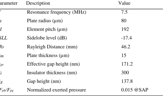
Table 2.2: The Parameters and specs of the designed 7.5 MHz centered CMUT

Parameter Description Value

f Resonance frequency (MHz) 7.5 a Plate radius (µm) 80 d Element pitch (µm) 192 SLL Sidelobe level (dB) -17.4 R0 Rayleigh Distance (mm) 46.2 tm Plate thickness (µm) 15

tge Effective gap height (nm) 171.2

ti Insulator thickness (nm) 300

tg Gap height (nm) 137.8

Fpb/Fpg Normalized exerted pressure 0.015 @SAP

(30)

12

Chapter 3 Simulations Results

The simulations done for this work were mainly done in Advanced Design Systems (ADS) and k-wave where the specification and limitations were according to DiPhAS such as the clock rate, voltage levels and other specifications. In ADS, the transient analyses were done with the clock rate of 480 MHz which is the clock rate for transmission in DiPhAS, therefore the time domain resolution was set to 2.083 ns. The excitation voltages used for the simulations were 10 VPP and 150 VPP to assess the difference in response and all the time at half the frequency of the desired acoustic frequency. Considering the fabrication limitations, for the k-wave simulations, the grid sizes were set as 32 µm while the gap height was set to 138 nm. As in [13], the Rayleigh Bloch waves have an effect to the array since the array size is much larger than the operating wavelength therefore this phenomenon was also considered in the simulations [14].

For simulation resulting purposes, three cells were considered in the array to reflect the major operational differences between the cells of different regions as presenting results of all 256 cells would be impossible. Therefore, one cell from outermost corner cells, one cell from center and one cell from the side were considered for analysis. The operational differences were mostly due to the mutual radiation impedance and effect of the rigid baffle around the cells [11].

(31)

13

The cells’ responses from the electrical input such as Harmonic balance and Transient analysis were done in ADS and the responses were then fed into the k-wave to analyze the focused transmission, beam forming and radiation pattern. The workflow shown in figure 3.2 better illustrates the work going into the simulation section.

Figure 3.2: Simulation flow diagram

3.1 Harmonic Balance Analysis

This simulation was done to analyze the frequency response of the CMUTs in the array in an unbiased mode of operation with excitation of 75 Vac. The analysis was done from the three cells mentioned above even though all the cells in the array were all excited in phase. The use of lumped element model enabled us to perform this analysis on ADS which allowed us to simulate the non-linear array device without having to use nonlinear simulation tools which would take a long time.

The output pressure of the CMUT array was observed with a second harmonic in the range of 1 MHz to 15 MHz with a step size of 50 kHz and according to these results, the peak pressure of 240.6 dB re 1µPa was observed at 6.36 MHz while at 7.5 MHz, a pressure of 232.8 dB re 1µPa was observed as seen in figure 3.3. The operation frequency was decided not to be at peak because of the narrow bandwidth and undesired transient response at this frequency, therefore it was decided to be at 7.5 MHz – at the right of the peak frequency.

(32)

14

Figure 3.3: Pressure output frequency response between 1 MHz – 20 MHz with 150 VPP and unbiased

The presence of Rayleigh Bloch waves on the surface of the transducer, introduce the difference in the velocities and hence pressure levels produced by individual cells [14][15] and this is due to the difference in radiation impedance observed by individual cells in the array. Therefore, the cells in the array each produced a slightly different pressure level as observed in the 1st cell where the pressure emitted was 440 kPa, 120th cell was 420 kPa while the 128th cell was 435 kPa all with excitation of 150 VPP. The maximum pressure difference at the operation frequency was calculated to be 0.7 dB re 1µPa. The spurious resonances due to the Rayleigh Bloch waves were visible with this analysis method, unlike in the biased mode it was evident that these resonances were at the right side of the operation frequency at around 11.5 MHz.

The frequency response of the particle velocity of the cells’ membranes was also analyzed between 1 MHz to 15 MHz at 150 VPP and the same peak frequency was observed. The difference in particle velocity between the cells in the array was however found to be more significant than the pressure levels between the cells which mostly explains the difference in power between the CMUT cells.

(33)

15

Figure 3.4: Particle velocity frequency domain analysis between 1 MHz – 20 MHz at 150 VPP

The difference between the particle velocities of cells at the peak frequency of 6.36 MHz was higher than the resonance frequency of 7.5 MHz just like in Pressure emitted. The particle velocities of cells at 6.36 MHz varied between 0.4 m/s to 0.8 m/s while at 7.5 MHz particle velocities varied between 1.11 m/s to 0.22 m/s with outer cells having the higher velocities than the inner cells.

The simulations for operating the array with a biasing voltage for the purpose of comparing the biased and unbiased operations were done. The VDC was calculated as 52.5 VDC, the calculated value enough to pre-deflect the membrane as much as ambient pressure deflects the unbiased cell membrane while the ac voltage to produce the same power was found to be 28.8 Vac. The harmonic balance simulations for the three dedicated cells were repeated for biased mode of operation and the results were exactly the same when plotted on top of the unbiased mode of operation frequency response results

(34)

16

3.2 Admittance Simulations

Conductance and Susceptance are another important characterizing entity telling how conductive the CMUT is at a specific frequency and voltage level. The conductance analysis also tells us more about the resonant frequency and charging up of the CMUT cell [16][4]. The conductance and susceptance are the reciprocal of the impedance and are calculated as follows [4];

𝐺 = 𝑅 {𝐼𝑖𝑛𝑝𝑢𝑡

𝑉𝑖𝑛𝑝𝑢𝑡} (3.1)

𝐵 = 𝐼 {𝐼𝑖𝑛𝑝𝑢𝑡

𝑉𝑖𝑛𝑝𝑢𝑡

} (3.2)

Operating a CMUT in an unbiased mode, introduces more nonlinearity nature which leads to changing of admittance values with change in input voltage. Therefore, the analysis was done with a voltage sweep from 10 VPP – 150 VPP with 20 and 40 VPP step size as seen on figure 3.7 and Appendix A.

(35)

17

Figure 3.6: Admittance values at 150 VPP

More admittance plots for this section are attached in the Appendix A which were all used to plot the admittance response to the change in the input voltage at 7.5 MHz with unbiased mode of operation as shown in the next plot.

(36)

18

3.3 Transient response

Transient analysis with a sinusoidal signal was done for the three dedicated cells to analyze the magnitude and behavior of pressure transmitted and well as the membrane displacement behavior at acoustic resonance frequency, 7.5 MHz and electrical resonance of 3.75 MHz with two different voltage levels, 10 VPP and 150 VPP. These excitation voltages were considered for simulation as they are the minimum and maximum output voltages of DiPhAS, and the transmission length was specified at 4 𝜇𝑠 which is the maximum transmit phase length for DiPhAS [4].

Figure 3.8: Transient analysis at 10 VPP and 3.75 MHz input signal

As the above plot shows, three cells were simulated with voltage input of 10 VPP at 3.5 MHz and the pressure output of three cells were observed at 7.5 MHz almost the same seen with different color codes peaking at 1933 Pa at steady state.

(37)

19

Figure 3.9: Transient analysis at 150 VPP and 3.75 MHz input signal

After observing the individual CMUT output pressure, the steady state membrane displacement was observed with 75 VPP sinusoidal input signal and the normalized steady state membrane displacement was found to be 0.1072.

Figure 3.10: Normalized steady state membrane displacement at 7.5 MHz with 150 VPP input voltage at 3.75 MHz

(38)

20

Since with the unbiased mode of operation the entire gap height was available for maximum swing gap, this meant that the maximum normalized membrane displacement is 0.806 as seen in the calculation below, the displacement achieved by 150 VPP was nowhere near maximum displacement.

max 𝑛𝑜𝑟𝑚𝑎𝑙𝑖𝑧𝑒𝑑 𝑑𝑖𝑠𝑝𝑙𝑎𝑐𝑒𝑚𝑒𝑛𝑡 = 𝑡𝑔

𝑡𝑔𝑒 = 0.806 (3.3)

To achieve the maximum allowable displacement, which is the gap height, the CMUT must be excited with the MVM [17][4] voltage which is 300 VPP calculated in chapter 2. Driving the CMUT cell beyond this voltage, the CMUT membrane will be touching the substrate which would increase the backing loss so better to be avoided [4].

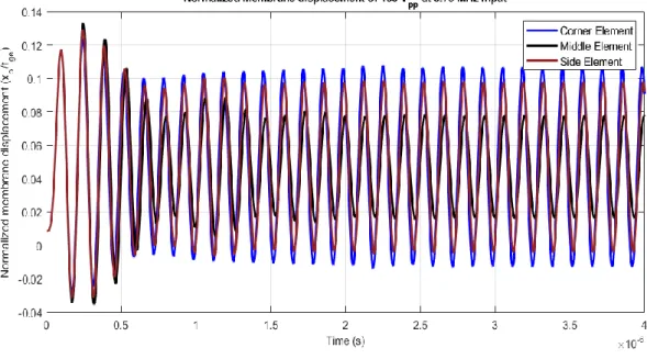
Figure 3.11: The steady state normalized membrane displacement at 298.4 VPP and 3.75 MHz input signal

The maximum normalized membrane displacement was found to be achieved only in the first cycle of the input while it dropped to about 0.4 for the following cycles. To maintain the maximum displacement, it would take giving a ramp input at 376 VPP but then that would allow a tapping motion of the membrane - bouncing back from the substrate periodically which is not desired.

(39)

21

Figure 3.12: The steady state output pressure from each CMUT cell excited at MVM, 298.4 VPP and at resonance frequency

The pressure emitted by each CMUT cell was observed for when the CMUT cells were sinusoidally excited with at the MVM, 300 VPP at the resonance frequency, 3.75 MHz and the steady state maximum pressure was observed at 1.673 MPa with 7.5 MHz acoustic signal as seen in the figure 3.12.

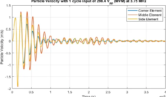
The particle velocity was also analyzed from the three dedicated cells at the MVM with only one cycle of a sinusoidal signal of 3.75 MHz and the velocity profile observed was of 2 cycles at 7.5 MHz with peak velocity of 1.231 m/s.

Figure 3.13: Particle velocity profile observed with one cycle signal of 300 VPP and 3.75 MHz

(40)

22

3.4 Tone Burst Signal Transmission

Transmission with ultrasonic transducers for biomedical imaging is mostly done a with tone burst signal [18] and for that reason it was necessary to perform simulations of transmission with a gaussian-enveloped tone burst signal of a few cycles to inspect the array response and behavior when transmitted with different voltages. The tone burst response was analyzed at three different voltage levels, 10 VPP, 150 VPP and 372.3 VPP (MVM), for Pressure emitted, particle velocity and membrane displacement.

The gaussian-enveloped sinusoidal tone burst signal of 5 cycles with amplitude of 10 VPP was generated at 3.75 MHz and from the three cells analyzed the transient response is shown below with an acoustic signal of 10 cycles resulting twice the input frequency, 7.5 MHz and peak pressure of 2255 Pa.

Figure 3.14: Transient response of 5-Cycle Gaussian-enveloped tone burst signal of 10 VPP at 3.75 MHz

Then the gaussian-enveloped sinusoidal tone burst signal of 5 cycles with amplitude of 150 VPP was generated at 3.75 MHz and a similar response was recorded with an increased output peak pressure 2.3 kPa with 10 VPP to 498.1 kPa.

(41)

23

Figure 3.15: Transient response of 5-Cycle Gaussian-enveloped tone burst signal of 150 VPP at 3.75 MHz

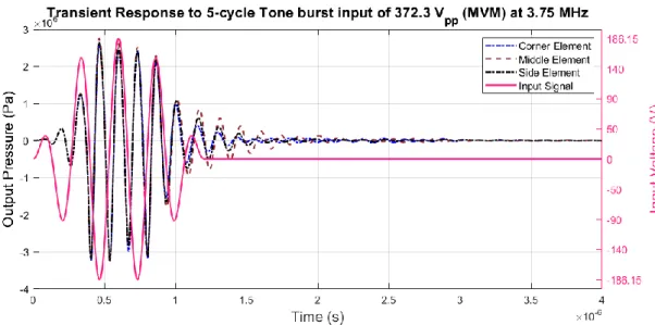
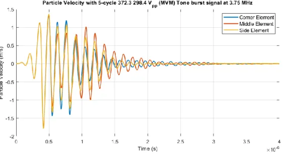
Finally, the gaussian-enveloped sinusoidal tone burst signal of 5 cycles with amplitude of 372.3 VPP which is the MVM was generated at 3.75 MHz and peak output pressure was observed to have marginally increased to 2.764 MPa. The normalized membrane displacement was also analyzed for this input voltage and noted to be 0.8 very close to the maximum achievable displacement and similar to the one found in chapter 3.4. The particle velocity at MVM was analyzed as well and found to peak at 1.362 m/s.

Figure 3.16: Transient response of 5-Cycle Gaussian-enveloped tone burst signal of 372.3 VPP at 3.75 MHz

(42)

24

Figure 3.17: Normalized membrane displacement analyzed at 372.3 VPP of 5-cycle Gaussian-enveloped tone burst signal

Figure 3.18: Particle velocity profile analysis at 372.3 VPP of 5-cycle Gaussian-enveloped tone burst signal. Peak observed at 1.362 m/s

(43)

25

3.5 Radiation Pattern Simulations

Radiation pattern is a very important property of a transmitter as it describes the pattern of the pressure radiated into the medium and was among the starting point in the designing of this transducer array. So far, we have been analyzing performances of individual cells in the array which even though were affected by other cells in the array but could not tell us much on the array’s performance. The radiation pattern simulation tells us how the transducer radiates in the medium and this had to be done on a FEM simulation tool which in this case, the k-wave MATLAB toolbox was used [19]. For the k-wave simulation, a very accurate environment had to be created in a k-wave workspace for the accuracy of the simulation results; that included designing the CMUT array, the medium, the receiver and the simulation space. However, since FEM simulations usually take long, an optimization was to be found between the accuracy and simulation time [20].

The CMUTs was designed using the grid points (voxel) of size 160 𝜇𝑚 x 160 𝜇𝑚. This voxel dimension was chosen based on the diameter of the CMUT which is 160 𝜇𝑚 and in each voxel there were smaller 5x5 cube grids of 32 𝜇𝑚 x 32 𝜇𝑚 . Having smaller grids improves the accuracy and this 32 𝜇𝑚 was chosen from the minimum feature size in the array which was the spacing between successive CMUT cells. The transducer was then a 16 x 16 of the 160 𝜇𝑚 x 160 𝜇𝑚 voxels.

(44)

26

The radius of the 3-D simulation space was then designed based on the Rayleigh distance in such a way the simulation space should be smaller than the Rayleigh distance to make sure the sensors were placed in the near field. Since each sensor cell was one voxel defined above, the enough sensors to be placed radially around the transducer at the Rayleigh distance were 1406 and to be sure we were well within the beamformable region, 1024 sensors were used. The symmetry of the Azimuth plane was used to reduce the simulation time, hence only 512 sensor voxels (equal to 16.384 mm) were used to provide results of 1024 sensors with short time. 10 voxels from each plane were set as Perfectly Matched Layers (PML) to avoid scattering of the acoustic waves from the boundary due to impedance difference between layers of simulation and far field [4]. The medium was set as water, by matching the properties such as density, speed of sound, nonlinearity coefficient and attenuation.

The ultrasonic source was set as dipole since the exert force on the surrounding medium causing about the physical membrane displacement.

Figure 3.20: Simulation space created in k-wave with the transducer located at X=0 and the sensor voxels as well as PML voxels placed radial to the transducer at 15.744 mm [4]

(45)

27

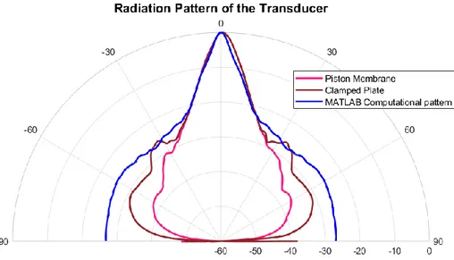
For transmission, the time-domain results obtained from 1 cycle of tone burst sinusoidal excitation with 10 VPP at 3.75 MHz in ADS for the individual cells were fed into the corresponding CMUT cells respectively for a volumetric transmission analysis. The transmission was done with 1 ns step sizes for 32 𝜇𝑠 and in order to use 1 ns step sizes, the results from ADS had to be interpolated. Two operational modes were simulated, as a piston membrane and as a clamped plate which best emulates the CMUT operation. For the piston membrane, the pressure distribution across the voxel was uniform while for the clamped plate, the pressure distribution through the membrane was not uniform but obeyed membrane deflection profile seen in chapter 2. The pressure values received from each of the 81 sensors from each transmission mode were used to plot the radiation patterns and compared with the computational radiation pattern with MATLAB formed by using the maximum pressure values obtained directly from the ADS simulation.

Figure 3.21: Radiation Patterns formed in k-wave Vs. the computational radiation pattern (dB re 1Pa)

(46)

28

3.6 Beamforming and Focusing

Beamforming is another property of CMUT arrays which allows the user to focus the pressure and a specific pressure and steer it as per the need. Beamforming is created by introducing specific transmission time delays to specific CMUT cells depending on the focus point location from the transmitting array and the center of the transducer. Focusing the beam at four angle points normal to the center of the transducer were considered; 0o, 15o, 30o, and 60o and each channel’s respective time delays for all those angle points were calculated using the equation (3.6) [21].

𝜏

_𝑛

= 𝑟 −

√(𝑥𝑟−𝑥𝑛)2+𝑧𝑟2

𝑐0

+ 𝑡

0

(

3.4

)

where 𝑟 is the distance from the center of the transducer to the point of focus, 𝑥_𝑛 is the distance between the center of transducer to the center of CMUT of interest and 𝑡₀ being the fictitious value to avoid negative values or very large delay values. The points of focus were only chosen to be in the elevation plane, which is the plane for the sensors, the points in azimuth plane were not considered to avoid complex computations.

After calculating the transmission delay times of each cell for a specific point, the pressure outputs obtained from 1 cycle of tone burst sinusoidal signal of 10 VPP at 3.75 MHz in ADS were fed in the k-wave space with their transmission respective time delays. The beamforming analysis was performed four times with different focusing locations mentioned above and the same 81 sensors were used to record the pressures.

It was observed that with the increase in angle of focus from the normal (0o), the peak pressure decreased and this is due to the diffraction limited focus [22], a phenomenon which implies that as the angle of focus increases, the total area of transmission increases hence sparse energy distribution.

(47)

29

Figure 3.22: The beamforming at points of interest, 0o_{, 15}o_{, 30}o_{, and 60}o _{from the} normal along with the plane wave transmission

3.7 Power and Intensity

Mechanical Power and Intensity of the transducer are other important characterization for a transducer which in this work, the calculation for Power of the emitted pressure were done with equation (3.7) [23]. Since mechanical power is the radiated power by the CMUT into the medium, the power of the whole transducer was calculated by superposing the powers by individual CMUTs.

𝑊_{𝑚𝑒𝑐ℎ} = 𝑅𝑒𝑎𝑙{𝑓 ∙ 𝑢∗} (3.5)

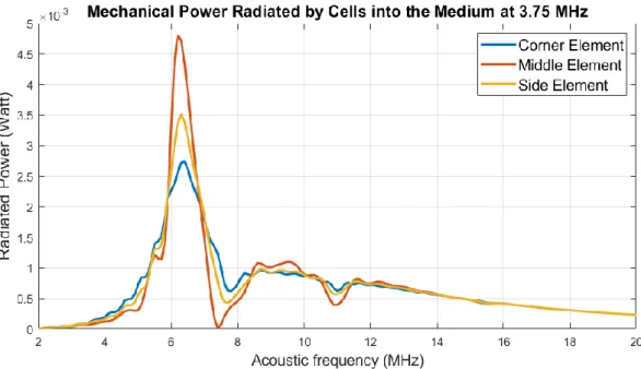
where 𝑓 is the force exerted on the receiver by the transducer and 𝑢∗_{is the} complex conjugate of the particle velocity. The power of pressure emitted by individual cells were calculated for the three dedicated cells from the values of pressure obtained in frequency domain analysis in ADS simulations. The power values recorded from the corner, side and middle cells at 7.5 MHz were 0.997 mW, 0.557 mW and 0.777 𝜇𝑊 respectively. The difference of power between the cells was huge and this was the result of the huge difference between particle velocities of CMUT cells.

(48)

30

Figure 3.23: Power of Individual CMUTs analyzed from the corner, middle and side elements

The total power radiated into the medium by the transducer was calculated by adding all the powers from the individual cells and the resulting plot was found to show that the total power at 7.5 MHz was 86.9 mW while at the peak frequency, the radiated power was 1.157 Watt.

(49)

31

To calculate the Intensity of the transducer, the time domain analysis will be used. In contrast to the calculation of power, the intensity is calculated by both the real and imaginary parts of the pressure and conjugate of particle velocity as in (3.8) [23].

𝐼 =

∑ 1 𝑡𝑎𝑣∫ |𝑓𝑖 × 𝑢𝑖 ∗_|𝑑𝑡 256 𝑖=1 𝑆

(3.6)

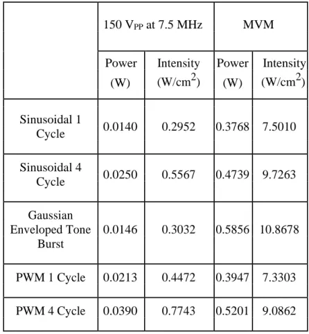
Where 𝑖 is the number of CMUT cells in the array, S is the total surface area of the 16 x 16 array transducer, 𝑓𝑖 being the force of individual CMUT cell and 𝑢_𝑖∗ the complex conjugate of particle velocity of individual CMUT. The intensities obtained from the time domain analysis discussed earlier are summarized in the table 3.3 below

Table 3.1: Power and Intensity of the transducer transmitting at 150 VPP and 7.5 MHz

150 VPP at 7.5 MHz MVM

Power Intensity Power Intensity

(W) (W/cm2) (W) (W/cm2) Sinusoidal 1 0.0140 0.2952 0.3768 7.5010 Cycle Sinusoidal 4 0.0250 0.5567 0.4739 9.7263 Cycle Gaussian Enveloped Tone 0.0146 0.3032 0.5856 10.8678 Burst PWM 1 Cycle 0.0213 0.4472 0.3947 7.3303 PWM 4 Cycle 0.0390 0.7743 0.5201 9.0862

(50)

32

Chapter 4 Fabrication

The fabrication of the CMUT array was performed a wafer scale and later on diced into separate chips of arrays. In this section, the fabrication processes will be discussed with the sequence of process flow. Mask designing will be discussed first, then the etching of the cavity will come next followed by deposition of bottom electrode and insulation layers. The wafer bonding will be discussed next before Flip-Chip bonding and sealing processes.

4.1 Mask Design

The designing of the mask was done after considering a few things discussed in the designing of the CMUT array itself and the fabrication facility limitations. Considering the pitch was designed to be 192 𝜇𝑚, the 256 cells were arranged in square manner of size 16 x 16 making sure the designed pitch is constant throughout. Since shadow mask was going to be used to this purpose and not the chrome masks, the electrical pads were determined to be 500 x 500 𝜇𝑚 which is a feasible dimension for a shadow mask. These pads were ideally located and in a square manner with gaps of 250 𝜇𝑚 in such a way they would allow enough space for fanning out the wires to their respective pads by keeping the wires as short as possible. Keeping the wires short was to avoid higher resistances due to long wires which would result to power losses [4].

Since the minimum fabricable wire width in our cleanroom facilities is 3 𝜇𝑚 and spacing of 3 𝜇𝑚 [4] and as discussed in designing chapter earlier, that 27 𝜇𝑚 gap would be needed to accommodate maximum of 4 wires while fanning out the wires to the pads, the pitch of 192 𝜇𝑚 of the CMUTs would leave 32 𝜇𝑚 gap which would allow that. The designed mask is in figure 4.1 below.

Designing, fabrication and post- fabrication characterization of half-frequency driven 16 x 16 waterborne transmit CMUT array

DESIGNING, FABRICATION AND

POST-FABRICATION CHARACTERIZATION OF

HALF-FREQUENCY DRIVEN 16 X 16

WATERBORNE TRANSMIT CMUT ARRAY

By

Yusuph Abubakar Abhoo

February 2021

ABSTRACT

DESIGNING, FABRICATION AND POST-FABRICATION

CHARACTERIZATION OF HALF-FREQUENCY DRIVEN

16 X 16 WATERBORNE TRANSMIT CMUT ARRAY

ÖZET

YARI FREKANSTA SÜRÜLEN SUALTI 16 X 16 ELEMANLI

CMUT DIZININ DIZAYNI, FABRIKASYONU VE

FABRIKASYON SONRASI KARAKTERIZASYONU

Acknowledgements

Contents

1

2

3

4

5

6

List of Figures

List of Tables

Chapter 1

Introduction

Chapter 2

The Design of the CMUT Array

2.1 Background on CMUT Cell and Array

Designing

2.2 Designing of the CMUT and the Array

2.2.1 CMUT cell radius, the pitch and the Rayleigh

distance

2.2.2 CMUT cell thickness membrane

𝑓 =

=

2.2.3 CMUT cell gap height, insulator thickness and

Collapse voltage

Chapter 3

Simulations Results

3.1 Harmonic Balance Analysis

3.2 Admittance Simulations

3.3 Transient response

3.4 Tone Burst Signal Transmission

3.5 Radiation Pattern Simulations

3.6 Beamforming and Focusing

𝜏

= 𝑟 −

+ 𝑡

(

)

3.7 Power and Intensity

𝐼 =

Chapter 4

Fabrication

4.1 Mask Design