Analysis of Lagrangian lower bounds for a graph partitioning problem

This article was downloaded by: [139.179.72.198] On: 25 October 2017, At: 07:04 Publisher: Institute for Operations Research and the Management Sciences (INFORMS) INFORMS is located in Maryland, USA

Operations Research

Publication details, including instructions for authors and subscription information: http://pubsonline.informs.org

Analysis of Lagrangian Lower Bounds for a Graph

Partitioning Problem

Gajendra K. Adil, Jay B. Ghosh,

To cite this article:

Gajendra K. Adil, Jay B. Ghosh, (1999) Analysis of Lagrangian Lower Bounds for a Graph Partitioning Problem. Operations Research 47(5):785-788. https://doi.org/10.1287/opre.47.5.785

Full terms and conditions of use: http://pubsonline.informs.org/page/terms-and-conditions

This article may be used only for the purposes of research, teaching, and/or private study. Commercial use or systematic downloading (by robots or other automatic processes) is prohibited without explicit Publisher approval, unless otherwise noted. For more information, contact [email protected].

The Publisher does not warrant or guarantee the article’s accuracy, completeness, merchantability, fitness for a particular purpose, or non-infringement. Descriptions of, or references to, products or publications, or inclusion of an advertisement in this article, neither constitutes nor implies a guarantee, endorsement, or support of claims made of that product, publication, or service.

© 1999 INFORMS

Please scroll down for article—it is on subsequent pages

INFORMS is the largest professional society in the world for professionals in the fields of operations research, management science, and analytics.

ANALYSIS OF LAGRANGIAN LOWER BOUNDS FOR A GRAPH

PARTITIONING PROBLEM

GAJENDRA K. ADIL

Department of Mechanical and Industrial Engineering, University of Manitoba, Winnipeg, Canada

JAY B. GHOSH

Faculty of Business Administration, Bilkent University, Ankara, Turkey, [email protected]

(Received September 1996; revisions received April 1997, December 1997; accepted February 1998)

Recently, Ahmadi and Tang (1991) demonstrated how various manufacturing problems can be modeled and solved as graph partitioning problems. They use Lagrangian relaxation of two different mixed integer programming formulations to obtain both heuristic solutions and lower bounds on optimal solution values. In this note, we point to certain inconsistencies in the reported results. Among other things, we show analytically that the first bound proposed is trivial (i.e., it can never have a value greater than zero) while the second is also trivial for certain sparse graphs. We also present limited empirical results on the behavior of this second bound as a function of graph density.

A

recent paper by Ahmadi and Tang (1991) demon-strates how various manufacturing problems such as the formation of group technology cells, the loading of tools or operations on a bank of identical flexible ma-chines, and the design of VLSI circuits can be effectively modeled as partitioning problems on an undirected graph. This latter problem essentially involves dividing a graph into a specified number of nonempty components such that the total weight of all edges spanning two distinct components is minimized. For its solution, Ahmadi and Tang propose two different mixed integer programming formulations and their Lagrangian relaxations. The relax-ations yield heuristics as well as lower bounds on the opti-mal solution value. The reported computational results seem to indicate that the heuristics and the lower bounds both perform reasonably well.

In this note, we point to several inconsistencies in the earlier work. We first show analytically that, while the first formulation is correct, the bound that it yields is trivial in that it can never have a positive value. We then observe that the second formulation is not valid but the bound derived from it still is. However, we go on to show that even a stronger version of this bound (which is derived after appropriately correcting the formulation) is also triv-ial for a class of sparse graphs. Finally, we report the results of a limited empirical study, which trace the strength of the second bound as a function of graph den-sity.

1. PROBLEM DEFINITION

We are given an undirected graph G⫽ (N, A), where N is an index set of the nodes numbered 1 through N and A is a set of node pairs representing the edges. If there exists an edge between nodes i and j, i, j 僆 N and i ⬍ j, then the

pair (i, j) denotes that edge. Associated with each edge (i,

j), (i, j)僆 A, is a weight wij, wij⬎ 0.

We let (N1, . . . , NM) be an M-way partition of N for any

M, 2 聿 M 聿 N, and consider it feasible if for all k, 1 聿

k 聿 M, the cardinality 兩Nk兩 of Nk satisfies the inequalities

1聿 兩Nk兩 聿 c (where c, c 肁 1, is a specified size limit). The

partition divides G into M components such that a compo-nent Gk, 1 聿 k 聿 M, is given by Gk ⫽ (Nk, Ak), where

Ak⫽ {(i, j)⬊(i, j) 僆 A and i, j 僆 Nk}. The cutset C induced

by this partition is the set of the edges in A that span two distinct components and is given by C⫽ A ⫺ 艛1聿k聿M Ak.

The objective in the graph partitioning problem is to find a feasible partition which minimizes ¥(i, j)僆Cwij.

Note that the graph partitioning problem is strongly NP-hard (Garey and Johnson 1979). Also note that it admits a feasible partition if and only if N 聿 Mc, and further that the Ahmadi-Tang formulations do not guarantee that an optimal partition contains exactly M nonempty compo-nents unless N⬎ (M ⫺ 1)c. For our purposes, we will thus assume that (M⫺ 1)c ⬍ N 聿 Mc.

2. FIRST FORMULATION AND RELAXATION

Define xikto be 1 if node i, i僆 N, belongs to component

k, 1聿 k 聿 M, and 0 otherwise. Similarly, define yijto be 1

if nodes i and j, (i, j)僆 A, belong to two different compo-nents. The first Ahmadi-Tang mixed integer programming formulation—call it (IP1) and its solution value V(IP1)—is as follows: V(IP1)⫽ min

冘

共i, j兲僆A wijyij subject to

冘

1聿k聿Mxik⫽ 1 for all i, i 僆 N, (1)

Subject classifications: Manufacturing: cell formation, tool loading, VLSI design. Networks/graphs: partitioning. Programming, integer: Lagrangian relaxation. Area of review: MANUFACTURINGOPERATIONS.

785

Operations Research 0030-364X/99/4705-0785 $05.00

Vol. 47, No. 5, September–October 1999, pp. 785–788 䉷 1999 INFORMS

冘

i僆Nxik⭐ c for all k, 1 ⭐ k ⭐ M, (2)

yij ⭓ xik⫺ xjk for all i, j, 共i, j兲 僆 A, and all k, 1 ⭐ k

⭐ M, (3)

xik僆 兵0, 1其 for all i, i 僆 N, and all k, 1 ⭐ k ⭐ M, (4)

yij ⭓ 0 for all i, j, 共i, j兲 僆 A. (5)

A Lagrangian relaxation of (IP1), call it (LR1␭), is

obtained by dualizing the constraint set (3) through the use of multipliers ␭ijk, (i, j) 僆 A and 1 聿 k 聿 M, such

that ␭ijk 肁 0. It is not necessary for us to write (LR1␭)

explicitly; the interested reader may refer to the Ahmadi and Tang (1991) paper. It suffices to observe that (LR1␭)

separates into two subproblems: a trivial one involving the yij and another involving the xik, which is a simple

transportation problem. Let V(LR1␭) be the value of

an optimal solution to (LR1␭) for the given multiplier

vec-tor ␭. The Lagrangian dual of (IP1)—call it (LD1) and its solution value V(LD1)—maximizes V(LR1␭) over all␭.

It is well known (see, for example, Fisher 1981 or Nemhauser and Wolsey 1988) that V(LR1␭)聿 V(LD1) 聿

V(IP1). The Ahmadi and Tang (1991) paper finds a solution to (LD1) using a subgradient optimization algorithm. Let V(LD1) be the solution value delivered by that algorithm. Clearly, V(LD1) 聿 V(LD1) 聿 V(IP1).

Now consider the continuous relaxation of (IP1), call it (LP1), where the 0-1 constraint set, (4), is replaced by the following:

0⭐ xik⭐ 1 for all i, i 僆 N, and all k, 1 ⭐ k ⭐ M. (6)

Let V(LP1) be the optimal solution value of (LP1). We now give the following result.

RESULT 1. V(LD1) 聿 V(LP1) ⫽ 0 for any G as long as

N聿 Mc.

PROOF. We prove the result by giving a feasible solution to (LP1) that has a solution value equal to 0 (i.e., it also happens to be optimal). This solution is:

xik⫽ 1/M for all i, i 僆 N, and all k, 1 ⭐ k ⭐ M, and

yij⫽ 0 for all i, j, 共i, j兲 僆 A.

It is trivially seen that the above solution satisfies the con-straint sets (5) and (6). It is similarly easy to see that it also satisfies (1) and (3). To see that it satisfies (2) as well, note that the LHS of (2) equals N/M and that this, under the stated condition (which is needed for the existence of a feasible partition anyway), is less than or equal to c (i.e., the RHS).

Let us now return to (LR1␭). It is evident that (LR1␭)

exhibits the so-called integrality property (see Fisher 1981 or Nemhauser and Wolsey 1988, again), i.e., V(LR1␭) does

not decrease when (4) is replaced with (6). As a

conse-quence of this property, we must have V(LD1)⫽ V(LP1). Hence, V(LD1)聿 V(LD1) 聿 V(LP) ⫽ 0. □

Thus, the lower bound derived from the first Ahmadi-Tang formulation cannot have a positive value and be of any use in an exercise such as the performance evaluation of a heuristic. This finding contradicts the computational results reported in the Ahmadi and Tang (1991) paper, sixth column of their Table 1.

3. SECOND FORMULATION AND RELAXATION

This time retain the xik but remove the yij. Instead, define

zijkto be 1 if nodes i and j, i, j 僆 N, belong to the same

component k, 1聿 k 聿 M, and 0 otherwise. For notational convenience, define the set Diof the neighboring nodes of

node i, i僆 N, as Di⫽ { j⬊(i, j) or ( j, i) 僆 A}. After minor

modifications (which are needed for clarity), the second Ahmadi-Tang mixed integer programming formulation— call it (IP2) and its solution value V(IP2)—can be written as follows: V(IP2)⫽ min

冘

共i, j兲僆A wij

冋

1⫺

冘

1聿k聿M zijk

册

, subject to

冘

j⬎i, j僆Di zijk⫹

冘

j⬍i, j僆Di zjik⭐ 共c ⫺ 1兲 xik

for all i, i僆 N, and all k, 1 ⭐ k ⭐ M, (7)

zijk 僆 兵0, 1其 for all i, j共i, j兲, 僆 A, and all k, 1 ⭐ k ⭐ M,

(8) and (1) and (4) as above.

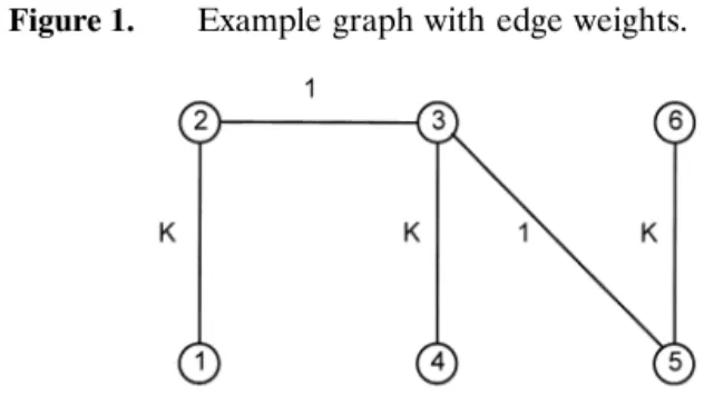
The above formulation is, however, incorrect. To see this, refer to Figure 1, which shows a 6-node graph with weights on the edges (the same graph used by Ahmadi and Tang (1991)). Suppose that M ⫽ 2 and c ⫽ 3. The true optimal solution value is K⫹ 1, given, for instance, by the partition ({1, 2, 6}, {3, 4, 5}). However, the solution given by x11⫽ x21⫽ x32⫽ x42⫽ x52⫽ x62⫽ 1 and z121⫽ z342⫽

z352⫽ z562⫽ 1 (with all the other variables set equal to 0)

satisfies constraints (1), (4), (7), and (8), and is thus feasi-ble with respect to (IP2). But this solution represents the infeasible partition ({1, 2}, {3, 4, 5, 6}) which yields a better-than-optimal solution value of 1.

Figure 1. Example graph with edge weights. 786 / ADIL ANDGHOSH

To correct (IP2), we replace (7) and (8) with the con-straint sets (9), (10), and (11) shown below, and call the resulting problem (IP2C) and its solution value V(IP2C):

冘

j⬎i, j僆Nzijk⫹j⬍i, j僆N

冘

zjik⭐ 共c ⫺ 1兲 xik

for all i, i僆 N, and all k, 1 ⭐ k ⭐ M, (9)

zijk ⭓ xik⫹ xjk⫺ 1

for all i, j, i, j僆 N and i ⬍ j, and all k, 1 ⭐ k ⭐ M, (10)

zijk 僆 兵0, 1其

for all i, j, i, j僆 N and i ⬍ j, and all k, 1 ⭐ k ⭐ M.₍₁₁₎ (IP2C) thus has the same objective function as (IP2) but comprises the constraint sets (1), (4), (9), (10), and (11). Notice that in (9) the sum is taken over all (i, j) such that i,

j僆 N and i ⬍ j, in contrast to (7) where the sum is taken only over (i, j)僆 A, to ensure that a partition’s size limit is properly enforced. Similarly, (10) is added to ensure that

zijkis 1 if and only if xikand xjkare both 1. Finally, notice

that (11) in (IP2C) can in fact be replaced by its continu-ous relaxation, which is given below:

0⭐ zijk⭐ 1 for all i, j, i, j 僆 N and i ⬍ j,

and all k, 1⭐ k ⭐ M. (12)

We now discuss the Lagrangian relaxation of (IP2) as obtained in the Ahmadi and Tang (1991) paper, where the constraint set (7) is dualized using multipliers␮ik, i 僆 N

and 1 聿 k 聿 M. (Again, we do not write the relaxation explicitly; the interested reader may refer to Ahmadi and Tang 1991.) We simply note that it separates into two subproblems: a trivial one involving the zijk and another

involving the xik that contains only GUB constraints. By

our convention, we call this relaxation (LR2␮) and its

op-timal solution value V(LR2␮) for a given multiplier vector

␮. The associated dual problem is called (LD2) and its solution value V(LD2). The solution value returned by the subgradient optimization algorithm is similarly called V(LD2).

It is easy to show at this point that, although (IP2) is incorrect, V(LR2␮), V(LD2) and V(LD2) remain valid

lower bounds on the optimal solution value V(LP2C) of the continuous relaxation (LP2C) of (IP2C), which is ob-tained by replacing (4) with (6) and (11) with (12). Notice also that (LR2␮), with only GUB constraints, exhibits the

integrality property mentioned earlier. This implies that V(LD2) ⫽ V(LP2) and thus that V(LD2) 聿 V(LD2) ⫽ V(LP2)聿 V(LP2C) 聿 V(IP2C).

We now proceed to analyze the quality of the Lagrang-ian lower bound obtainable from the correct formulation (IP2C) by dualizing in the same manner as in (IP2), i.e., by dualizing (9) and (10) in this case. Notice that the integral-ity property still holds, because the relaxed problem con-tains only GUB constraints as before. Thus, if we let (LD2C) with solution value V(LD2C) be the Lagrangian dual of (IP2C), then V(LD2C) ⫽ V(LP2C). Because

V(LD2)聿 V(LD2) 聿 V(LP2C), any upper bound we de-rive on V(LP2C), or equivalently V(LD2C), can be im-posed upon the Ahmadi-Tang bound V(LD2) as well. Let ␦i, ␦i⫽ 兩Di兩, be the degree of node i, i 僆 N. Now define

the maximum degree of graph G to be ⌬, where ⌬ ⫽ maxi僆N{␦i}. We now give a result for the case when⌬ is

sufficiently small.

RESULT 2. V(LD2) 聿 V(LP2C) 聿 0 for any G with ⌬ 聿

c⫺ 1.

PROOF. Once again, we prove the result by providing a feasible solution to (LP2C) with value 0 (which may not be optimal). This solution is:

xik⫽ 1/M for all i, i 僆 N, and all k, 1 ⭐ k ⭐ M,

zijk ⫽ 0 for all i, j, i, j 僆 N,

i⬍ j and 共i, j兲ⰻA, and all k, 1 ⭐ k ⭐ M, and

zijk ⫽ 1/M for all i, j, 共i, j兲 僆 A, and all k, 1 ⭐ k ⭐ M.

This solution clearly satisfies (6) and (12). It is also easy to see that it satisfies (1). The RHS of (10) is 2/M⫺ 1 聿 0 (since M肁 2), the LHS is 0 or 1/M, and thus it is satisfied as well. The LHS of (9) is␦i/M 聿 ⌬/M, the RHS is (c ⫺

1)/M, and it too is satisfied under the stated condition. Finally, the solution value can be seen to be 0. □

Notice that the maximum degree⌬ of graph G is at least as much as its average degree (which is proportional to the graph’s density). A high ⌬ does not necessarily imply a dense graph, but a low ⌬ implies a sparse graph. Thus, Result 2 indicates that the Lagrangian lower bound is go-ing to be trivial for a class of sparse graphs when ⌬ is smaller than c. But we do not know yet what happens to V(LP2C), or equivalently V(LD2C), for sparse graphs in general. We, therefore, undertake a small computational study. Our study complements the one in the Ahmadi-Tang paper, which is performed over relatively dense graphs.

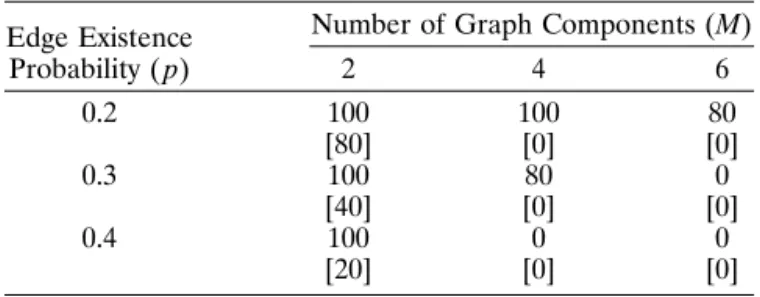
Let p be the probability that an edge exists between nodes i and j, i, j僆 N; notice that p is the expected density of a randomly generated graph. Keeping c fixed at 6, we consider M⫽ 2, 4, and 6, and p ⫽ 0.2, 0.3, and 0.4. This leads to 9 cases; in each case, N⫽ Mc as in Ahmadi and Tang (1991). Ten graphs are generated randomly for each case, with the edge weights drawn from a uniform distribu-tion over (1, 10). (LP2C) is solved for each graph (using a commercial LP solver on a UNIX workstation). We want to find out what percentage of the times in each scenario V(LP2C) is nonpositive. Table 1 records our results and shows what percentage of the times in each scenario the maximum degree⌬ of the graph is less than c, i.e., when V(LP2C) is provably nonpositive. Notice that, for a fixed expected density p, if M is increased, we get more and more positive values for V(LP2C). A similar behavior is observed if, for a fixed M (and thus N), the expected den-sity p is increased.

787 A

4. CONCLUSION

We show that the first Ahmadi-Tang Lagrangian lower bound is trivial. The second bound, however, holds prom-ise for graphs that are sufficiently dense. It appears that the Ahmadi-Tang computations cover such graphs only. The reported results are encouraging. Also, despite the poor quality of the associated lower bound, the first La-grangian heuristic continues to perform reasonably well, as has been indicated by Ahmadi and Tang (1991) and as has

been independently observed by us in a small computa-tional study. To sum up, in using the Ahmadi-Tang ap-proach, one could choose the first Lagrangian heuristic and the second lower bound. However, in case of the lat-ter, one would have to pay close attention to the density of the graphs under consideration.

ACKNOWLEDGMENTS

The authors benefitted significantly from the helpful com-ments of the associate editor and two anonymous referees during the revision of this note.

REFERENCES

Ahmadi, R. H., C. S. Tang. 1991. An operation partitioning problem for automated assembly system design. Oper.

Res. 39 824–835.

Fisher, M. L. 1981. The Lagrangian relaxation method for solving integer programming problems. Management Sci.

271–18.

Garey, M. R., D. S. Johnson. 1979. Computers and

Intractabil-ity. Freeman, New York.

Nemhauser, G. L., L. A. Wolsey. 1988. Integer and

Combina-torial Optimization. Wiley, New York.

Table 1. Test of the second Lagrangian lower

bound with the component size limit (c) fixed at 6.

Percentage of Cases where the Bound is Trivial: Actual [Provable]

Edge Existence Probability ( p)

Number of Graph Components (M)

2 4 6 0.2 100 100 80 [80] [0] [0] 0.3 100 80 0 [40] [0] [0] 0.4 100 0 0 [20] [0] [0]

788 / ADIL ANDGHOSH