Selçuk J. Appl. Math. Selçuk Journal of Vol. 8. No.2. pp. 25 - 36 , 2007 Applied Mathematics
Maximum Likelihood Estimation and Confidence Intervals of System Reliability for Gompertz Distribution in Stress-Strength Models1
Bu˘gra Saraço˘glu and Mehmet Fedai Kaya
Department of Statistics, Faculty of Art and Science, Selcuk University, 42031, Konya, Turkey
e-mail:bugrasarac@ selcuk.edu.tr,fkaya@ selcuk.edu.tr
Received : April 4, 2007
Summary. A stress-strength model defines life of a component which has strength and is subjected to stress In this paper, we consider the estimation problem of = ( ) when ˜ ( 1) and ˜ ( 2) are independent with known. can be considered to be the reliability of a system and is known to be stress-strength reliability. The maximum likelihood estimate of is derived and various distributional properties of this estimator is discussed. Exact and asymptotic confidence intervals for are constructed. Also a simulation study is performed to investigate the coverage probabilities of these intervals.
Key words:Coverage probability; Stress-strength reliability; Gompertz distri-bution; Minimum variance unbiased estimation; Maximum likelihood estima-tion; Confidence interval
1. Introduction
The term "stress-strength reliability" in statistical literature typically refers to the quantity ( ). This term states the reliability of a system of strength subjected to a stress The system fails if the applied stress exceeds its strength. Thus the quantity is known to be the stress-strength reliability of the system and is typically denoted by . In other words, the stress-strength reliability of the system is the probability that the system is strong enough to overcome the stress imposed on it. The problem arises in some fields, for example, in biometry, represents a patient’s remaining years of life if treated with drug and represents the patient’s remaining years of life if treated
1This study is a part of philosophy of doctora (Ph.D) thesis titled "Estimation of System
Reliability for some Distributions in Stress-Strength Models" , Bu˘gra Saraço˘glu, submitted by Selcuk University Graduate School of Natural and Applied Sciences, 2007.
with drug . If the choice is left to the patient, person’s deliberations will center on whether ( ) is less than or greater than 1/2 (Ali and Woo, 2005a, 2005b).
Some authors have considered different choices for stress and strength distrib-utions. The stress-strength reliability and it’s estimation problems for several distributions are discussed in the works of Church and Harris (1970) , Downton (1973), Woodward and Kelley (1977), for the family of normal distributions, Tong (1974, 1975a, 1975b), Sathe and Shah (1981), Chao (1982) for the family of exponential distributions, Beg and Singh (1979) for the family of pareto dis-tributions, Awad and Gharraf (1986) for the family of Burr XII disdis-tributions, Constantine et al. (1986), and Ismail et al. (1986) for the family of gamma dis-tributions, McCool (1991), Kundu and Gupta (2006) for the family of weibull distributions, Surles and Padgett (1998, 2001), Raqab and Kundu (2005) for the family of burr X distributions, Ali and Woo (2005a, 2005b) for the family of levy and p-dimensional rayleigh distributions„ Kundu and Gupta (2005) for the family of generalized exponential distributions and Mokhlis (2005) for the family of burr III distributions. Recently, Kotz et al. (2003) have presented a review of all methods and results on the stress-strength model in the last four decades.
This paper is organized as follows; In Section 2, the stress-strength reliability is derived underlying The distribution. In Section 3, maximum likeli-hood estimate (MLE) of the stress-strength reliability () is obtained and vari-ous distributional properties of this estimator is discussed. Also, mean squares error (MSE) of the these estimates are compared. In Section 4, exact and as-ymptotic confidence intervals for the stress-strength reliability are constructed and a simulation study is performed to investigate the coverage probabilities of these intervals as well.
2. Stress-Strength Reliability
Let be the strength of a system and be the stress acting on it. and are the random variables from with parameters (1 1) and (2 2) respectively. That is, the probability density functions and the cumulative dis-tribution functions of and are, respectively
(2.1) () = 1exp (1) exp©−1−11 [exp (1) − 1]ª 0 1 0 1 0
(2.2) () = 1 − exp©−1−11 [exp (1) − 1]ª and (2.3) () = 2exp (2) exp © −2−12 [exp (2) − 1] ª 0 2 0 2 0
(2.4) () = 1 − exp©−2−12 [exp (2) − 1]ª
where 1 and 2 are known parameters and also 1 and 2 are unknown para-meters. Then is = ( ) = Z ∞ 0 ( ) () = ∞ Z 0 ∙ 1 − exp ½ −2 2 (2− 1) ¾¸ 11exp ½ −1 1 (1− 1) ¾ = 1 − exp ½ 1 1 +2 2 ¾ Z∞ 11 exp ( −2 2 µ 1 1 ¶21) − (2.5)
If we write the identity given by Eq.(2.6) in the right hand side of the integral given by Eq.(2.5) (2.6) exp ( −2 2 µ 1 1 ¶21) = ∞ X =0 (−1)( 22)(11)21 !
The final form of Eq.(2.5) is rearranged as follows;
= 1 − exp ½ 1 1 +2 2 ¾ × ∞ X =0 (−1)(22)(11)21 ! (2.7) × ⎡ ⎢ ⎣Γ (21+ 1) − Z11 0 (21)− ⎤ ⎥ ⎦
where Γ () is a gamma function. If we write the identity given by Eq.(2.8) in the right hand side of the integral given by Eq.(2.7),
(2.8) −= ∞ X =0 (−1) !
then Eq.(2.7) is rearranged as follows; = 1 − exp {11+ 22} × ∞ X =0 (−1)( 22)(11)21 ! (2.9) × " Γ ((21) + 1) − ∞ X =0 (−1)( 11)(21)++1 ((21) + + 1) ! #
If 1= 2= then is in the form given as follows;
= ( ) = ∞ Z 0 ( ) () = ∞ Z 0 ∙ 1 − exp ½ −2(− 1) ¾¸ 1exp ½ −1(− 1) ¾ = 2 1+ 2 (2.10)
3. Estimation of Stress-Strength Reliability 3.1. Maximum Likelihood Estimation
Let 1 2 and 1 2 be the two independent random sam-ples taken from the distribution with parameters ( 1) and ( 2) respectively and let be known. Then, likelihood and log-likelihood function based on the above samples are given as follows;
(θ; x y) = 1exp à X =1 ! exp à −1 X =1 (− 1) ! 2 exp à X =1 ! × exp " −2 X =1 ( − 1) # (3.1) and
(θ; x y) = log 1+ X =1 − 1 X =1 (− 1) + log 2+ X =1 − 2 X =1 ( − 1) (3.2)
respectively, where θ = (1 2) is the parameter vector and subsequently the associated gradients are found as follows;
(θ; x y) 1 = 1 − 1 X =1 ( − 1) = 0 (θ; x y) 2 = 2 − 1 X =1 ( − 1) = 0
Hence MLEs of the parameters 1 and 2 are obtained by
ˆ 1= −1P =1( − 1) (3.3) ˆ 2= −1P =1(− 1) (3.4)
respectively. Using the invariance properties of the maximum likelihood esti-mation, b1that is the MLE of the is obtained as follows;
(3.5) b1= b2 b1+ b2 Let = −1P=1(− 1) and = −1P =1( − 1) Then b1 is calcu-lated by (3.6) b1= b2 b1+ b2 = +
The following method can be used to find the distribution of b1 Let = and we consider the below transformation
: ⎧ ⎨ ⎩ 1= + = ; then ( = = 1 (1 − 1) and its jacobian is as follows;
= ¯ ¯ ¯ ¯ ¯ ¯ (1 − 1) + 1 2(1 − 1)2 1(1 − 1) 2(1 − 1)2 0 −2 ¯ ¯ ¯ ¯ ¯ ¯= − 3(1 − 1)2 so that || = n3(1 − 1)2 o
Since 0 implies 1 0 we have
1 = µ 1 (1 − 1) ¶ || = µ 1 (1 − 1) ¶ () || = 1 2 −1 1 Γ () Γ () (1 − 1)+1 1 ++1exp ½ − 11 (1 − 1)− 2 ¾ with 0 and 0 1 1 Then the distribution of b1can be found as follows;
1(1) = 12 1−1 Γ () Γ () (1 − 1)+1 ∞ Z 0 1 ++1 exp ½ − 11 (1 − 1)− 2 ¾ = Γ ( + ) Γ () Γ () µ 1 2 ¶ 1−1(1 − 1)−1 × ½ 1 − 1 µ 1 − 1 2 ¶¾−(+) (3.7)
with 0 1 1 For 0, moment of b1is given by
³b1´= ∞ Z 0 1 1(1) = Γ ( + ) Γ( + ) Γ ( + + ) Γ () µ 1 2 ¶ × 21 µ ( + + ) + + 1 − 1 2 ¶ (3.8)
where (n d ) is the generalized hypergeometric function. This function is also known as Barnes’s extended hypergeometric function. The definition of (n d ) is as follows; (3.9) (n d ) = ∞ P =0 Q =1 Γ (+ ) Γ−1() Γ ( + 1) Q =1 Γ (+ ) Γ−1()
where n = [1 2 ], is the number of operands of n, d = [1 2 ] and is the number of operands of d. The above generalized hypergeometric function is quickly evaluated and readily available in standard software pro-grammes such as Maple. For more details see Gradshteyn et al. (2000). By replacing = 1 in Eq.(3.8) the expected value of b1 can be found as follows;
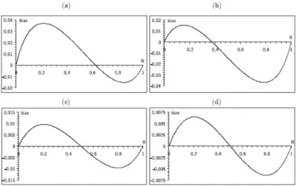
(3.10) ( b1) = ( + ) µ 1 2 ¶ 21 µ ( + 1 + ) + + 1 1 −1 2 ¶ Fig. 1 shows the graphs of bias of the MLE as a function of the true reliability for these cases: (a) =5, =3, (b) =3, =5, (c) =10, =10 and (d) =15, =15. MLE has relatively more bias for lower reliability values than higher ones when and MLE has relatively more bias for higher reliability values than lower ones when . Also bias of the MLE tends to decrease in the case that the total sample size, + increases.
Fig. 1.The Bias curves of the MLE, for (a) = 5, = 3, (b) = 3, = 5, (c) = 10, = 10 and (d) = 15, = 15 Using Eq. (3.8), the variance of the b1can be obtained as follows;
³b1 ´ = ³b21 ´ −³³b1 ´´2 = ( + 1) ( + ) ( + + 1) µ 1 2 ¶ × 21 µ ( + 2 + ) + + 2 1 −1 2 ¶ − ½ ( + ) µ 1 2 ¶ 21 µ ( + 1 + ) + + 1 1 −1 2 ¶¾2 (3.11) 4. Confidence intervals 4.1. Exact confidence interval
Let 1 2 and 1 2 be the two independent random sam-ples taken from the distribution with parameters ( 1) and ( 2) respectively and let be known. Recall that = −1P
=1( − 1) and = −1P
=1( − 1) are independent gamma random variables with para-meters ( 1) and ( 2) respectively. Also it can be easily shown that 21 and 22 are two independent chi-square random variables with 2 and 2 degrees of freedom respectively. Thus b1 in Eq.(3.5) could be rewritten as ³
1 + b1b2 ´−1
Using Eq.s(2.10), (3.3), (3.4) and (3.6) the MLE of 1is ob-tained as follows; (4.1) b1= µ 1 +1 2 ¶−1 where (4.2) = (1 − )
is an F distributed random variable with (2 2) degrees of freedom. could be written as follows; (4.3) = 1 − ³ b 1−1− 1´
Using as a pivotal quantity, a (1 − ) 100% exact confidence interval for is obtained by (4.4) Ã (2)(22) (2)(22)+ b1−1− 1 (1−2)(22) (1−2)(22)+ b−11 − 1 !
where ()() is the th quantile of the F distribution with ( ) degrees of freedom.
The other option is to find a 100(1 − )% lower confidence bound for . Then ( 1) is a 100(1 − )% one-sided confidence interval for Hence for any 0 1, a 100 (1 − ) % lower confidence bound for is
(4.5) ()(22) ()(22)+ b1−1− 1
4.2. Asymptotic confidence interval
Let 1 2 and 1 2 be the two independent random samples taken from the distribution with parameters ( 1) and ( 2) re-spectively. The MLE b1in Eq.(3.5) is asymptotically normal with mean and variance (4.6) 2 X =1 2 X =1 1 2 −1
where −1is the ( )th element of the inverse of the Fisher’s information matrix which is given by = ⎡ ⎢ ⎣ 21 0 0 22 ⎤ ⎥ ⎦
(Rao, 1965). Thus, the asymptotic variance of b1 is as follows; (4.7) + b 2 1 ³ 1 − b1 ´2
Hence an asymptotic (1 − ) 100% confidence interval for is obtained by (4.8) Ã b 1− 1−2 r + b1 ³ 1 − b1 ´ b1+ 1−2 r + b1 ³ 1 − b1 ´!
where 1−2 is the 1 − 2th quantile of the standard normal distribution. 4.3. Simulation study
To study the performance of the confidence intervals, 50000 samples are simu-lated from the distribution with the values of parameters (1 2 ) = (1 2 1), (1 5 1), (5 5 1) and different sample size of and . It is important to examine how well our proposed methods work for constructing confidence intervals. In this section, the approximate confidence intervals based on asymp-totic properties of the MLEs are compared with the exact confidence intervals in terms of coverage probabilities. The simulation results are shown in Table 1 and Table 2. The coverage probabilities of the exact confidence intervals for are all close to the desired level of 0.95, but the coverage probabilities of the approximate confidence intervals for are not so close to 095. The coverage probabilities of the approximate confidence intervals are close to 095, virtually for ≥ 50 and ≥ 50.
Table 1. Coverage probabilities for the proposed methods and the MLEs of for various values of (1 2 ) (n fixed, m increased)
Table 2. Coverage probabilities for the proposed methods and the MLEs of for various values of (1 2 ) (m fixed, n increased)
References
1.Ali, M.M., Woo, J., 2005a. Inference on reliability P(YX) in the Levy distribution. Math. Comp. Modell. 41, 965—971.
2.Ali, M.M., Woo, J., 2005b. Inference on reliability P(YX) in a p-dimensional rayleigh distribution. Math. Comp. Modell. 42, 367-373.
3.Awad, A.M., Gharraf, M.K., 1986. Estimation of P(YX) in the Burr case: A comparative study, Commun. Statist. Simul. Comp. 15, 2, 389-403.
4.Beg, M.A., Singh, N., 1979. Estimation of P(YX) for the pareto distribution. IEEE Trans. Reliab. 28, 5, 411-414.
5.Chao, A., 1982. On Comparing Estimators of P(YX) in the exponential case, IEEE Trans. Reliab. 31, 4, 389-392.
6.Church, J.D., Harris, B., 1970. The estimation of reliability from stress strength relationships. Technometrics 12, 49-54.
7.Constantine, K., Karson, M., 1986. Estimators of P(YX) in the gamma case. Commun. Statist. Simul. Comp. 15, 365-388.
8.Downton, F., 1973. On the estimation of P(YX) in the normal case. Technometrics 15, 551-558.
9.Gradshteyn, I.S., Ryzhik, I.M., 2000. Tables of Integrals, Series, and Products, Academic Press, San Diego, CA.
10.Ismail, R., Jeyaratnam, S., Panchapakesan, S., 1986. Estimation of P(XY) for gamma distributions. J. Statist. Comput. Simul. 26, 253-267.
11.Kotz, S., Lumelskii, Y., Pensky, M., 2003. The Stress-Strength Model and its Generalizations: Theory and Applications, World Scientific Publishing, Singapore. 12.Kundu, D., Gupta R.D, 2005. Estimation of P(YX) for the generalized exponen-tial distribution. Metrika 61 3, 291—308.
13.Kundu, D., Gupta R.D, 2006. Estimation of P(YX) for weibull distributions. IEEE Trans. Reliab. 55, 2, 270-280.
14.McCool, J.I., 1991 Inference on P(YX) in the Weibull case Commun. Statist. Simul. Comp. 20, 1, 129-148.
15.Mokhlis, N.A., 2005. Reliability of a stress-strength model with Burr Type III distributions, Commun. Statist.Theory Meth. 34, 7, 1643-1657.
16.Raqab M.Z., Kundu, D., 2005. Comparison of different estimators of P(YX) for a scaled Burr type X distribution. Commun. Statist. Simul. Comp. 34, 2, 465—483. 17.Sathe Y.S., Shah, S.P. 1981. On estimation P(YX) for the exponential distribu-tion. Commun. Statist. Theory Meth. A10, 1, 39—47.
18.Surles, J.G., Padgett, W.J., 1998. Inference for P(YX) in the Burr type X model. J. Appl. Statist. Sci. 7, 4, 225—238.
19.Surles, J.G., Padgett, W.J., 2001. Inference for reliability and stress-strength for a scaled Burr-type X distribution. Lifetime Data Analy. 7, 187—200.
20.Tong, H., 1974. A note on the estimation of P(YX) in the exponential case. Technometrics 16, 625.
21.Tong, H., 1975. A note on the estimation of P(YX) in the exponential case. Technometrics 16, 625.
22.Tong, H., 1975. A note on the estimation of P(YX) in the exponential case Technometrics 17, 395.
23.Woodward, W.A., Kelley, G.D., 1977. Minimum variance unbiased estimation of P(YX) in the normal case Technometrics 19, 95—98.