Identification of theranostic gene markers in cancers and prognostic validation in colorect al cancer

i

IDENTIFICATION OF THERANOSTIC GENE

MARKERS IN CANCERS AND PROGNOSTIC

VALIDATION IN COLORECTAL CANCER

A THESIS SUBMITTED TO

THE GRADUATE SCHOOL OF ENGINEERING AND SCIENCE OF BILKENT UNIVERSITY

IN PARTIAL FULFILLMENT OF THE REQUIREMENTS FOR THE DEGREE OF

MASTER OF SCIENCE IN

MOLECULAR BIOLOGY AND GENETICS

By

Murat İşbilen

January, 2015

ii

IDENTIFICATION OF THERANOSTIC GENE MARKERS IN CANCERS AND PROGNOSTIC VALIDATION IN COLORECTAL CANCER

By Murat İşbilen January, 2015

We certify that we have read this thesis and that in our opinion it is fully adequate, in scope and in quality, as a thesis for the degree of Master of Science.

Assist. Prof. Dr. Ali OSMAY GÜRE

Assist. Prof. Dr. Özlen KONU

Assist. Prof. Dr. Aybar Can ACAR

Approved for the Graduate School of Engineering and Science:

Prof. Dr. Levent Onural Director of the Graduate School

iii

ABSTRACT

IDENTIFICATION OF THERANOSTIC GENE MARKERS IN

CANCERS AND PROGNOSTIC VALIDATION IN COLORECRAL

CANCER

M.Sc. in Molecular Biology and Genetics Advisor: Assist. Prof. Dr. Ali Osmay GÜRE

January 2015

Colorectal cancer (CRC) is the fourth most prevalent cancer type worldwide. Although the 5-year survival rate of CRC is higher than many cancer types, prediction of prognosis and identification of accurate biomarkers still maintain their importance for chemotherapy benefits, thus survival of the patients. Current techniques to identify biomarkers for clinical use are based on building models with multi-gene signatures. However, the accuracy rates of such signatures are not high enough due to heterogeneity of the tumors and low sensitivity of gene expression measurement techniques, although cell lines can be predicted very well with such signatures. There has also been sufficient evidence that multi-gene signatures may not be better predictors than random signatures with the same size. Therefore, in this study, we aimed to develop two R-based statistical analysis tools, SSAT and USAT, to identify single-gene expression markers for prognosis with chemotherapy benefit prediction power. We identified two genes, ULBP2 and SEMA5A, with SSAT and 6 genes, PTRF, TGFB1I1, DUSP10, KLF9, CLCN7 and CLDN3, with USAT for colon cancer and CRC, respectively. We were able to validate independent prognostic power of ULBP2 and SEMA5A in an independent cohort. However, we could only validate CLCN7 among 6 genes that we identified by USAT. Those results showed that SSAT may be a better tool to identify prognostic gene markers and USAT needs to

iv

be improved to identify better candidate genes. We could also reveal the chemotherapy benefit prediction power of ULBP2 and SEMA5A in CCLE and CGP drug databases, although these in silico results should be validated by in vitro experiments. We believe that the approach that we used in this study may pioneer the studies to develop commercial theranostic tools for clinical use in various types of cancer.

v

ÖZET

KANSERDE PROGNOZ VE KEMOTERAPİ FAYDASI TAHMİNİ

YAPABİLEN GEN BELİRTEÇLERİNİN BELİRLENMESİ VE

KOLOREKTAL KANSERDE PROGNOZ BELİRTEÇLERİNİN

DOĞRULAMA ÇALIŞMASI

Moleküler Biyoloji ve Genetik, Yüksek Lisans Tez Danışmanı: Yard. Doç. Dr. Ali Osmay GÜRE

Ocak 2014

Kolorektal kanser (KRK) dünyada en yaygın olan dördüncü kanser türüdür. KRK için 5 yıllık hayatta kalma oranı diğer kanser türlerinden daha yüksek olmasına rağmen prognoz tahmini ve yüksek tahmin gücü olan biyobelirteçlerin belirlenmesi hastaların tedavilerden faydalanabilmeleri ve hayatta kalabilmeleri için hala önemini korumaktadır. Klinikte kullanılacak biyobelirteçlerin belirlenmesi için günümüzde kullanılan teknikler çok genli listeler ile model oluşturmak üzerine kuruludur. Fakat, bu tür modeler hücre hatlarını güzelce ayırabilirken, tümördeki çeşitlilik ve gen ifadesini ölçen tekniklerin düşük duyarlılığı yüzünden tümör örneklerinde doğru tahmin oranları yeteri kadar yüksek değildir. Daha önceki yayınlanmış çalışmalar da gösteriyor ki, çok genli listeler eşit sayıda gen içeren rastgele gen listelerinden daha iyi ayrımlar yapamıyorlar. Bu sebeple, biz bu çalışmada, kemoterapi faydasını tespit edebilen tek gen prognoz belirteçleri belirlemek için, iki adet R tabanlı istatistiksel analiz programı (SSAT ve USAT) geliştirmeyi hedefledik. SSAT ile ULBP2 ve SEMA5A genlerini kolon kanseri için ve USAT ile PTRF, TGFB1I1, DUSP10, KLF9, CLCN7 ve CLDN3 genlerini KRK için aday prognoz belirteçleri olarak tespit ettik. ULBP2 ve SEMA5A genlerini bağımsız bir hasta grubunda diğer klinik parametrelerden bağımsız prognoz belirteçleri olarak doğruladık. Fakat,

vi

USAT ile belirlediğimiz aday genlerden sadece CLCN7 genini doğrulayabildik. Bu sonuçlar bize SSAT’ın aday prognoz belirteçleri belirlemek için daha iyi bir program olabileceğini ve USAT’ın daha iyi prognoz belirteçlerini tespit edebilmesi için geliştirilmesi gerektiğini gösterdi. Ayrıca CCLE ve CGP ilaç veritabanlarında ULBP2 ve SEMA5A genlerinin kemoterapi faydası tahmini yapabildiklerini de gösterdik. Fakat bu sonuçlar in vitro deneyler ile doğrulanmalıdır. Bu çalışmada kullandığımız yöntemlerin, klinikte kullanılabilecek, prognoz ve kemoterapi faydası tahmini yapabilen ürünlerin geliştirilmesi için yapılacak çalışmalara katkı sağlayacağına inanıyoruz.

vii

ACKNOWLEDGEMENTS

I am pleased to express my sincere gratitude to my tolerant and wise supervisor Dr. Ali Osmay Güre for his unique and persistent guidance and motivating and encouraging support throughout my M.Sc. project. I am very grateful to him that he provided me with many opportunities, by which I could improve my experimental, computational and analytical skills. I got experienced a lot under his precious supervision. It is an honor for me to be a member of his lab.

Secondly, I cannot thank enough Dr. Mithat Gönen, Dr. Cemal Deniz Yenigün and Dr. Koray Doğan Kaya. They taught me a lot about biostatistics and bioinformatics. They shared their precious time and experiences with me to contribute to my project.

I would like to extend my gratitude to Dr. Özlen Konu and Dr. Aybar C. Acar for their valuable feedbacks and guidance for the project. They provided me with new insights for the development of the project.

I also feel grateful to al AOG lab members for their friendly, kind and motivating behaviors in the course of the project. I would like to thank specifically Kerem Mert Senses for his informative and helpful attitudes when I got stuck in my project. He was like my elder brother. I also thank Secil Demirkol and Dr. Emre Dayanç very much. They did all the validation experiments for SSAT approach.

I would like to express my greatest and profound thanks to my Pakistani friends Muhammad Waqas Akbar and Umar Raza. Indeed, they were more like brothers to me rather than friends. They never made me feel alone in my life in Bilkent University. I am also very thankful to Gökhan Şentürk, Sevi Durdu and Ali Cihan. Gökhan was Dr. Gure’s senior student. He got a funding from TUBITAK and supported my project financially. Sevi started this project and Ali developed it. They also helped me a lot to improve and finalize the project.

Finally, I declare that I owe all my achievements to my beloved parents Hüseyin and Sevda İşbilen, my dear brothers Sezer and Kadircan İşbilen and my beautiful fiancée Melike Öndeş. My parents worked hard throughout their lives to build a bright future for me and my brothers. They supported every decision I made and made me feel powerful against every difficulty I encountered. I felt my family’s prayers and motivational supports in every situation.

viii TABLE OF CONTENTS 1. IN TR OD U CTION ... 1 1.1.PROGNOSTIC SIGNATURES ... 2 1.2.PREDICTIVE SIGNATURES ... 4 1.3.AIM ... 5

2. M A TER IALS AN D M ETH OD S ... 6

2.1.COHORTS AND DATASETS ... 6

2.1.1. Tumor Microarray Datasets ... 6

2.1.2. Ankara Cohort ... 6

2.1.3. Cell Line Microarray Datasets ... 6

2.2.EXPERIMENTAL PROTOCOLS ... 7

2.2.1. Tumor Homogenization and RNA Extraction ... 7

2.2.2. DNase Treatment and cDNA Synthesis ... 7

2.2.3. qPCR Experiments ... 8

2.3.STATISTICAL ANALYSES ... 9

2.3.1. Hierarchical Clustering Analyses ... 9

2.3.2. Global Effectiveness Profiles ... 9

2.3.3. Comparison of Drug Response between Subtypes ... 10

2.3.4. Survival Analyses ... 10

2.3.4.1. Discretization of Expression Values ... 10

2.3.4.2. SSAT ... 10

2.3.4.3. USAT... 11

2.3.4.3.1. Model Generation ... 11

2.3.4.4. Log-Rank with Multiple Cut-offs ... 13

2.3.5. Gene Expression Profile Comparison of Cohorts ... 13

3. R ESU LTS ... 14

3.1.IDENTIFICATION OF CHEMOTHERAPEUTIC SUBTYPES IN CANCERS CELL LINES... 14

3.1.1. Hematological Cancer Cell Lines ... 14

ix

3.1.3. Colorectal Cancer Cell Lines... 19

3.2.IDENTIFICATION OF PROGNOSTIC SUBTYPES IN TUMORS ... 20

3.2.1. SSAT ... 21

3.2.1.1. Gene Selection for Validation ... 23

3.2.1.2. Validation of ULBP2 and SEMA5A as Prognostic Gene Markers ... 24

3.2.1.3. Prediction of Chemotherapy Benefit with ULBP2 and SEMA5A ... 26

3.2.1.4. Conclusion ... 28

3.2.2. USAT ... 28

3.2.2.1. True Positivity of USAT ... 29

3.2.2.1.1. USAT with Different Models ... 29

3.2.2.2. False Positivity of USAT ... 30

3.2.2.3. Gene Selection for Validation... 30

3.2.2.4. Validation of Microarray Expression with qPCR Expression ... 32

3.2.2.5. Validation of USAT Results... 33

3.2.2.5.1. Log-Rank Analysis with Multiple Cut-off Values (LRMC) ... 34

3.2.2.6. Further Analyses to Explain Opposite Results ... 38

3.2.2.6.1. Identification of CRC Subtypes like Ankara Cohort ... 38

3.2.2.6.2. Comparison of Cohorts by Correlation between Genes... 41

3.3.CONCLUSION ... 42

4. D ISCU SSION ... 44

4.1.CHEMOTHERAPEUTIC SIGNATURES ... 44

4.1.1. Gene Signatures in Hematological Cancer Cell Lines ... 44

4.1.2. Gene Signatures in Breast Cancer Cell Lines ... 46

4.1.3. Gene Signatures in Colorectal Cancer Cell Lines ... 47

4.2.THERANOSTIC GENE SIGNATURES IN CRC ... 48

4.2.1. SSAT and USAT ... 49

4.2.1.1. Identification and Validation of Candidate Genes by SSAT ... 52

4.2.1.2. Identification and Validation of Candidate Genes by USAT ... 56

4.2.1.3. Further Analyses to Understand the Reasons Behind Opposite Results ... 59

4.3.CONCLUSION ... 62

x

LIST OF FIGURES

Figure 3.1: Classification of hematological cancer cell lines based on gene expression profile. ... 15 Figure 3.2: G lobal effectiveness of B ryostatin in CPG database. ... 16 Figure 3.3: H ierarchical clustering of breast cancer cell lines in CCLE and global effectiveness distribution of Lapatinib. ... 17 Figure 3.4: H ierarchical clustering of breast cancer cell lin es in CCLE (A ) and CG P (B ) databases based on 12-gene signature. ... 18 Figure 3.5: H ierarchical clustering of CR C cell lines in CCLE and CG P databases. ... 19 Figure 3.6: Com parison of IPA -3 response of CR C cell line sub-groups and global effectiveness of IPA -3. ... 20 Figure 3.7: Schematic representation of SSA T approach. ... 23 Figure 3.8: K aplan-M eier Curves for U LB P2, SEM A 5A and combina tion of both. 25 Figure 3.9: G lobal effect distribution of A Z628 (A ) and differential response of prognostic CR C sub-groups to A Z628 (B ). ... 27 Figure 3.10: Schematic representation of U SA T approach. ... 31 Figure 3.11: Concordance between qPCR and microarray expression of the genes selected for validation. ... 34 Figure 3.12: LR M C analysis of PTR F in Ankara cohort. ... 36 Figure 3.13: LR M C analysis of the selected genes in G SE17 536, G SE41258 and A nkara cohort. ... 37 Figure 3.14: W TH C analysis of G SE17536 and LR M C analyses of selected genes for the clusters. ... 39 Figure 3.15: H ierarchical clustering of G SE17536 based on 48 -gene list and LR M C analyses of selected genes based on the clusters. ... 40

xi

Figure 3.16: Pearson r correlation heat-maps of the expression of the selected genes for A nkara cohort, G SE17536 and G SE41258. ... 41

xii

LIST OF TA BLES

Table 3.1: Clinical Characteristics and univariate CoxPH analysis results for G SE17536, G SE17537, G SE41258 and A nkara cohort. ... 22 Table 3.2: M ultivariate Cox proportional H azard regression results and corresponding statistics of selected genes in G SE17536 and G SE17537 datasets. .... 24 Table 3.3: Stepwise m ultivariate Cox proportional hazard regression results and corresponding statistics of prognosis separation by U LB P2 and SEM A 5A in A nkara cohort. ... 26 Table 3.4: N um ber of significant genes am ong 48 genes in U SA T m odels. ... 30 Table 3.5: R esults of U SA T analyses with continuous micro array expression values for G SE17536 and G SE41258. ... 32 Table 3.6: R esults of U SA T’s 12 M odels for G SE17536 and G SE41258. ... 33 Table 3.7: R esults of U SA T analyses with qPCR expression for A nkara cohort. ... 35

1

1. Introduction

Colorectal cancer (CRC) is one of the most prevalent cancer types worldwide, comprising around 10% of all cancer cases [1]. Although CRC is one of the most preventable cancer types as inappropriate eating habit, smoking and body fatness are the main risk factors for CRC, early diagnosis is still crucial for the survival of CRC patients [2, 3]. The patients who are diagnosed with TNM Stage I CRC have 90-95% 5-year survival rate after surgery, although the patients who are diagnosed with TNM Stage IV CRC have 5-10% 5-year survival rate [3]. Distant metastasis and local recurrence are the main reasons why CRC patients die due to cancer within 5 years after surgery.

The main treatment after surgery for CRC patients is adjuvant chemotherapy and radiotherapy to prevent recurrence. Whether CRC patients will be treated with adjuvant chemotherapy is determined according to histopathological characteristics of the resected tumors (infiltration to inner layers, metastasis to lymph nodes etc.) [4] and single molecule markers like p53/p21 expression, KRAS/BRAF mutations MSI etc. [5]. However, those characteristics do not provide opportunity to prediction of chemotherapy outcome, although they give insights into the prognosis of CRC patients. It has been shown that most stage III CRC patients benefit from chemotherapy, although the benefit of adjuvant chemotherapy in stage II CRC patients is still debatable [6]. In other words, many stage II and III CRC patients may be exposed to adverse effects of chemotherapy from which they would not benefit. Therefore, it is crucial to determine which stage II and III CRC patients to treat and not to treat with adjuvant chemotherapy in order to advance the treatment of CRC.

Recently, the common tendency in molecular biology to determine the benefit of any clinical use is to identify genomic signatures containing many parameters, like gene

2

expression, mutations etc. Identification of such markers requires high-throughput data, which has been published recently on databases, like Gene Expression Omnibus (GEO), in an increasing manner. Studies based on gene expression have been popular in the field of identification of biomarkers due to the advances in high-throughput gene expression measurement techniques, like microarray, next generation sequencing etc. Microarray data is one of the easiest high-throughput data to acquire, because of the publication rate and ease of handling. Therefore, a high amount of research have been conducted based on gene expression data to generate hypotheses or validate results. It has also been of great interest in identification of gene expression markers for clinical parameters, like prognosis, benefit of chemotreatment etc.

1.1. Prognostic Signatures

To date, many prognostic gene expression biomarkers have been identified for CRC. As reviewed by Schaeybroeck et al. [7], the first prognostic gene expression signature was a 23-gene signature, which was described by Wang et al. [8] in 2004 using two different approaches to distinguish between recurrent and relapse-free patients. They used split-sample method as their first approach by separating 74 stage II CRC patients into 36-patient training set and 38-36-patient test set. They selected 60 genes using training set and built a Cox model to predict recurrence in patients in the test set. In the second approach, they clustered all 74 patients by hierarchical clustering according to the expression of 17,616 genes and identified two distinct clusters. They assigned each patient sample into either cluster by the expression of most differentially expressed gene (Cadherin 17) between those clusters. Analyzing each cluster separately by split-sample method again, they selected 23 genes including Cadherin 17 to build a Cox model to predict recurrence. They report that the second approach successfully identified a gene expression signature with a prognostic value but the first approach did not [8].

3

Barrier et al. [9] also described a 30-gene tumor and 70-gene non-neoplastic mucosa prognostic signatures in 2005 using microarray expression data of 18 stage II and III (9 recurrent, 9 non-recurrent) CRC patient samples to predict recurrence. Their method consisted of two steps, one of which is the selection of the differentially expressed genes between relapse-free and recurrent samples and the other one is the recurrence prediction through k-nearest neighbor method. They determined the number of genes and the nearest neighbors by six-fold cross-validation. Barrier et al. [10] also used 50 stage II CRC patient samples to validate Wang et al.’s 23-gene prognostic signature using the same split-sample method. It was the first validation of a prognostic gene signature for CRC that was described by a completely independent group [7, 10].

O’Connell et al. [11, 12] developed Oncotype DX® as 12-gene prognostic signature to predict 3-year recurrence risk and 11-gene predictive signature to predict chemotherapy benefit in stage II CRC patients through recurrence and treatment scores using FFPE tissues [12]. They performed multivariate Cox Proportional Hazard Regression to determine the genes associated with recurrence and treatment benefit. Then, they generated a 4-step selection procedure to build models for recurrence risk and treatment benefit. They used 1,851 CRC patients from National Surgical Adjuvant Breast and Bowel Project (NSABP) and Cleveland Clinic cohorts [12]. They also validated their results by 1,436 stage II CRC patients from the QUASAR trial [13].

Salazar et al. developed ColoPrint as an 18-gene prognostic signature to predict recurrence in early stage CRC patients using fresh frozen tumor samples [14]. They used 188- and 206-patient CRC cohorts as discovery and validation sets. They used Kaplan-Meier method and Log-Rank test to determine the variables (e.g. gene expression, clinical parameters) associated with prognosis. They built also multivariate Cox models with the significant variables to find independent variables.

4

ColDx is another 634-gene signature to predict recurrence risk of stage II CRC patients and was developed by Kennedy et al. using FFPE tissues from 73 and 142 patients with recurrent and non-recurrent CRC patients [15]. They identified classifiers based on recursive feature elimination and partial least square classification. As a result, 10 repeats of five-fold cross validation showed that the 643-gene signature was the optimal for prognostic separation.

OncotypeDX®, ColoPrint and ColDx were three of prognostic gene expression signatures developed in recent years by large number of patients. OncotypeDX® is the only one which is commercially available. The others are currently undergoing clinical validation research. One of the disadvantages of these signatures is that they cannot calculate a treatment score for chemotherapy benefit. In fact, OncotypeDX® underwent a failed retrospective validation study for chemotherapy benefit [16]. Therefore, these signatures have no chemotherapy benefit prediction power even for the patients predicted in high risk group.

1.2. Predictive Signatures

There is no commercially available chemotherapy benefit signatures due to many reasons but one of the main reason is that prediction signatures developed by tumor samples have some bottlenecks like small clinical trial sample size and heterogeneity of tumors. It is also not possible to study many drugs at the same time and to determine the best drug for each individual in those trials. Therefore, high-throughput research settings were required to determine the chemotherapy treatment from which each patient can benefit most. For this reason, several cell line drug response databases were established; Cancer Cell Line Encyclopedia (CCLE) [17] and Cancer Genome Project (CGP) [18] are two of them. One of the main disadvantages of cell line drug databases are that the findings were evaluated under the assumption that cancer cell lines may represent tumors in terms of

5

chemotherapy response. Nevertheless, CCLE provides evidence that tumor samples resemble cell lines in terms of gene expression profile [17].

CCLE includes 947 cell lines originated from many known cancer types and screened for 24 drugs with different action of mechanisms, as CGP includes 789 cell lines screened for 138 drugs. Mutation data for specific genes, gene expression and chromosomal copy number data are also available in those databases. Analyses of combination of those data may reveal many molecular level interactions and provide with the identification of general biomarkers for chemotherapeutic response in cancers, as Barretina et al. [17] and Garnett et al. [18] published some gene expression and single-molecule markers for the benefit of some drugs. Therefore, these databases have the utmost importance for the analyses of predictive signatures and remain to be analyzed further.

1.3. Aim

In this study, we aimed to develop algorithms to identify independent prognostic markers with chemotherapy benefit prediction power. For that reason, we first used cell line databases to find subtypes of different cancer types with differential drug responses. Secondly, we tried to identify prognostic subtypes in tumors with gene signatures and single-gene lists using approaches both similar with and different than the ones that we used for cell lines. Thirdly, we tried to assess the chemotherapy benefit powers of identified prognostic genes.

6

2. Materials and Methods

2.1. Cohorts and Datasets

GSE17536, GSE17537 and GSE41258 microarray datasets were downloaded from GEO (“http://www.ncbi.nlm.nih.gov/geo”) and normalized with GC-RMA method using GeneSpring 12.0. Corresponding clinical data were downloaded from ArrayExpress (“http://www.ebi.ac.uk/arrayexpress”). GSE17536 and GSE17537 include the gene expression profiles of 177 and 55 fresh frozen colon cancer tumor tissues, respectively. GSE41258 includes gene expression profiles of 390 samples, 182 of which are colorectal cancer samples. It also includes 54 normal colon samples, 49 polyp samples and many normal and metastatic samples from liver and lung.

2.1.2. Ankara Cohort

Ankara cohort that includes fresh frozen tumor tissues of 47 colon and 37 rectal cancer patients were used as validation cohort. The samples were collected from the patients in … hospital and validated as tumor tissues by pathologists. The patients were followed for around 4 years and various clinical data were recorded.

2.1.3. Cell Line Microarray Datasets

GSE36133 [17] (CCLE database) and E-MTAB-783 [18] (CGP database) datasets were downloaded from ArrayExpress (“http://www.ebi.ac.uk/arrayexpress”) and normalized with RMA method using GeneSpring 12.0.

7

2.2. Experimental Protocols

2.2.1. Tumor Homogenization and RNA Extraction

The tumor samples were cut into small pieces on dry ice and 100 mg of each tumor sample were homogenized in 1 ml of TRIzol reagent. After homogenization, the samples were frozen and TRIzol reagent RNA extraction protocol (catalog number: 15596-018) was applied for each sample after all the samples were homogenized. The samples were centrifuged at 12,000 g for 10 minutes at 4°C to remove the insoluble content of the samples. After 5 minutes incubation at room temperature, 0.2 ml of chloroform was added to the samples. The samples were shaken vigorously for 15 seconds and incubated at room temperature for 3 minutes. They were centrifuged at 12,000 g for 15 minutes at 4°C and upper aqueous phase was removed and placed into a new tube. 0.5 ml of 100% isopropanol was added onto aqueous phase and incubated at room temperature for 10 minutes. The resulting mixture was centrifuged at 12,000 g for 10 minutes at 4°C. The supernatant was removed and the pellet was washed with 1 ml of 75% ethanol by vortexing briefly. The samples were centrifuged at 7,500 g for 5 minutes at 4°C and the wash was discarded. The RNA pellet was dried for around 10 minutes and resuspended in 100 µl nuclease-free water and incubated at 55°C for 10 minutes. The concentration of the samples were calculated by NanoDrop 1000 Spectrophotometer.

2.2.2. DNase Treatment and cDNA Synthesis

DNase treatment was applied to RNA samples by Life Technologies’ Ambion DNA-free Kit (catalog number: AM1906). The RNA samples were diluted so that the concentrations were 200 ng/µl and the experiment was performed with 60 µl reaction setup. 6 µl of 10X DNase buffer and 1.2 µl of rDNase I enzyme were added into 52.8 µl of RNA samples. After 20 minutes incubation at 37°C, 6 µl of resuspended DNase inactivation reagent was

8

added into the samples and incubated in room temperature for 2 minutes by mixing occasionally. The samples were centrifuged at 10,000 g for 1.5 minutes and the RNA was transferred to a new tube. The concentration of the samples were calculated by NanoDrop 1000 Spectrophotometer.

cDNA synthesis was performed by Thermo Scientific Fermentas RevertAid First Strand cDNA Synthesis Kit (catalog number: K1622). The RNA samples were diluted so that the concentrations were 500 ng/µl in the final reaction and the experiment was performed with 100 µl reaction setup. Master Mix was prepared for all samples at once with 20 µl of 5X reaction buffer, 5 µl of Ribolock RNase inhibitor, 10 µl of 10 mM dNTP mix and 5 µl of RevertAid M-MuLV Reverse Transcriptase enzyme for each sample. The reaction mixture included 55 µl of diluted RNA samples, 5 µl of random hexamer primer and 40 µl of Master Mix for each sample. Before addition of Master Mix, the samples with primers were incubated at 65°C for 5 minutes. The reaction took place under the conditions at 25°C for 5 minutes, 42°C for 60 minutes and 70°C for 5 minutes, in order.

2.2.3. qPCR Experiments

All qPCR reactions were run using TaqMan gene expression assays with 96-well plate format in 7500 Real-time PCR Systems. The best coverage MGB primer-probes with catalog number 4331182 were used for PTRF (Assay ID: Hs00396859_m1), TGFB1I1 (Assay ID: Hs00210887_m1), DUSP10 (Assay ID: Hs00200527_m1), KLF9 (Assay ID: Hs00230918_m1), CLCN7 (Assay ID: Hs01126462_m1) and CLDN3 (Assay ID: Hs00265816_s1). The best coverage MGB primer-probes with catalog number 4448892 were used for PCSK5 (Assay ID: Hs00196400_m1) and PLS3 (Assay ID: Hs00192406_m1).

The reaction mixture was comprised of 10 µl of TaqMan gene expression Master Mix, 1 µl of primer-probe, 7 µl of nuclease-free water and 2 µl of cDNA for each sample. The

9

initial reaction (holding stages) took place under the condition at 50°C for 2 minutes and 95°C for 10 minutes. The cycling stage reaction took place for 45 cycles under the condition at 95°C for 15 seconds and 60° for 1 minute.

Three experimental replicas were used for each gene of each sample. The mean cycle threshold (CT) values of three replicas were used as actual CT values for relative gene expression calculations. Relative gene expression values were calculated using 2-∆∆CT calculation, where

∆∆𝐶𝑇 = (𝐶𝑇_{𝑇𝑎𝑟𝑔𝑒𝑡}− 𝐶𝑇_{𝐺𝐴𝑃𝐷𝐻})

𝑆𝑎𝑚𝑝𝑙𝑒− (𝐶𝑇𝑇𝑎𝑟𝑔𝑒𝑡− 𝐶𝑇𝐺𝐴𝑃𝐷𝐻)𝑅𝑒𝑓𝑒𝑟𝑒𝑛𝑐𝑒

2.3. Statistical Analyses

2.3.1. Hierarchical Clustering Analyses

The hierarchical clustering analyses were performed with Cluster 3.0 with Euclidean distance and complete linkage method and visualized as heat-maps with dendograms with JTreeView. Standardized gene expression values were used for hierarchical clustering analyses. Whole Transcriptome Hierarchical analyses were performed by “hclust” function in R [19] with Euclidean distance and Ward method.

2.3.2. Global Effectiveness Profiles

The global effectiveness distributions of the drugs were visualized with boxplots for each cancer type included in CCLE and CGP databases using “boxplot” function in R. Normalized activity area and IC50 were used as drug sensitivity parameters in CCLE and CGP, respectively.

10

2.3.3. Comparison of Drug Response between Subtypes

The drug responses of two groups and more than two groups were compared student’s t-test and ANOVA, respectively, using “t.t-test” and “aov” functions in R. The drug response distributions of the groups were visualized as jitter plots using “stripchart” function in R.

2.3.4. Survival Analyses

All univariate survival analyses including Cox proportional hazard regression, maximally selected rank statistics and Log-Rank tests and Kaplan-Meier method were performed using “survival” package [20] in R. Stepwise multivariate Cox proportional hazard regression analyses were performed using IBM SPSS Statistics 19.

2.3.4.1. Discretization of Expression Values

Three types of expression values were used in survival analyses. Continuous expression values were used as they were generated by GC-RMA normalization of datasets using GeneSpring 12.0. Two types of categorical expression values were used in analyses. First, logarithmic gene expression values were divided into 8 different categories so that the expression values between 0 and 2 were category 1, the ones between 2 and 4 were category 2 and so on. The expression values above 14 were considered as category 8. The second categorical expression values contained two categories as high and low expression categories determined by Maxstat threshold values.

2.3.4.2. SSAT

After probeset normalization, all but one of the probesets that hit the same gene were eliminated so that the one with the highest coefficient of variance were used in survival analyses as the representative of the gene. The gene expression values were categorized into 8 groups, as explained in Discretization of Expression Values section. For each gene,

11

7 sequential expression thresholds were determined to compare the samples in the categories 1 vs. 2, 3, 4, 5, 6, 7 and 8; 1, 2 vs. 3, 4, 5, 6, 7 and 8 and so on with Log-Rank test. The genes with a p-values less than 0.05 were considered as significant for the given threshold.

2.3.4.3. USAT

All the probesets were analyzed with CoxPH, Maxstat and Log-Rank tests, with continuous and categorical expression values. In each test, the p-value threshold was 0.05. 12 different models were generated using combinations of the statistical tests and the expression types. The probesets that were significant in all the statistical tests at least in one model were considered as significant.

2.3.4.3.1. Model Generation

The models were generated by combining CoxPH, Maxstat and Log-Rank tests with continuous and categorical expression values. The explanation of generated models are as follows:

1. CC-MC-LC: Univariate CoxPH regression with continuous expression values, Maxstat with continuous expression values, Log-Rank with 2-category expression values.

2. CCS-MC-LC: Bivariate CoxPH regression with continuous expression values and stage, Maxstat with continuous expression values, Log-Rank with 2-category expression values.

3. CG-MC-LC: Univariate CoxPH regression with 8-category expression values, Maxstat with continuous expression values, Log-Rank with 2-category expression values.

12

4. CGS-MC-LC: Bivariate CoxPH regression with 8-category expression values and stage, Maxstat with continuous expression values, Log-Rank with 2-category expression values.

5. CC-MG-LG: Univariate CoxPH regression with continuous expression values, Maxstat with 8-category expression values, Log-Rank with 2-category expression values.

6. CCS-MG-LG: Bivariate CoxPH regression with continuous expression values and stage, Maxstat with 8-category expression values, Log-Rank with 2-category expression values.

7. CG-MG-LG: Univariate CoxPH regression with 8-category expression values, Maxstat with 8-category expression values, Log-Rank with 2-category expression values.

8. CGS-MG-LG: Bivariate CoxPH regression with 8-category expression values and stage, Maxstat with 8-category expression values, Log-Rank with 2-category expression values.

9. MC-C12-LC: Maxstat with continuous expression values, univariate CoxPH regression with 2-category expression values, Log-Rank with 2-category expression values.

10. MC-C12S-LC: Maxstat with continuous expression values, bivariate CoxPH regression with 2-category expression values and stage, Log-Rank with 2-category expression values.

11. MG-C12-LG: Maxstat with 8-category expression values, univariate CoxPH regression with 2-category expression values, Log-Rank with 2-category expression values.

13

12. MG-C12S-LG: Maxstat with 8-category expression values, bivariate CoxPH regression with 2-category expression values and stage, Log-Rank with 2-category expression values.

2.3.4.4. Log-Rank with Multiple Cut-offs

All the possible expression threshold values were determined for each probeset and Rank tests were performed for all these expression thresholds. For each probeset, the Log-Rank p-values were plotted for corresponding expression thresholds. Blue and red colors were used to express the direction of the association of the high expression of the genes with good and poor prognosis, respectively, based on the given thresholds.

2.3.5. Gene Expression Profile Comparison of Cohorts

Pearson’s correlation between the expression of the genes (probesets for microarray datasets and qPCR expression for Ankara cohort) were calculated within cohorts and shown with heat-maps.

14

3. Results

In this study, we first identified gene signatures that could differentiate between distinct cancer cell lines subtypes, which were sensitive and resistant to different drugs, using commonly used supervised and unsupervised clustering approaches. However, those approaches, by which gene signatures could be defined, did not work for tumors to find prognostic subtypes. Therefore, we decided to develop algorithms that could identify single gene markers, rather than signatures, which could define distinct prognostic subtypes. We developed Semi-supervised Survival Analysis Tool (SSAT) and Unsupervised Survival Analysis Tool (USAT) for the identification of prognostic gene markers in any cohort with high-throughput gene expression and clinical data. We performed SSAT and USAT analyses with three different CRC microarray datasets and tried to validate their results with a unique CRC cohort by qPCR.

3.1. Identification of Chemotherapeutic Subtypes in Cancers Cell Lines

We first aimed to identify a gene signature to find new genetic subtypes in hematological cancer cell lines, which exhibited differential drug response [21], rather than clinically-defined classification. We used gene expression and drug response data for hematological cancer cell lines from Cancer Cell Line Encyclopedia (CCLE) [17] and Cancer Genome Project (CGP) [18] to identify gene signatures for subtypes and drug response. According to hierarchical clustering with the expression of 1,000 most variant genes, we identified 8 distinct subtypes of hematological cancer cell lines in CCLE database and selected 400 of 1,000 genes as a signature, all of which were either positively or negatively correlated with any one of 8 clusters with a Pearson r more than 0.5 (Figure 3.1A-B). We also validated the expression pattern of each group identified in CCLE using CGP database with the

15

common cell lines in both databases. The heat-map in Figure 3.1C shows that the expression pattern of each cluster in CCLE was highly correlated with the counterpart in CGP according to our signature.

After we had showed that there had been similar clusters in both databases, we checked whether those clusters could define sensitive subgroups to drugs better than classical classification. We used other cancer types as reference to determine whether hematological

Figure 3.1: Classification of hematological cancer cell lines based on gene expression profile.

(A) Heat-map shows the expression profiles of hematological cancer cell lines clustered as

shown in clustering tree (B) based on the standardized expression of 400 genes in CCLE database. In the heat-map, red, green and black colors show high, low and intermediate gene expression, respectively. Each cluster in the three is defined by a color. (C) The heat-map shows the concordance of the clusters based on the expression profiles of 400 genes in CCLE and CGP databases. Red, blue and white colors present positive, negative and no correlation, respectively.

16

cancer clusters or classical subtypes were sensitive to a drug. Therefore, we compared each clusters or subtypes with each other, as well as other cancer types. We found out that new clusters of hematological cancers could identify sensitive cell lines to some drugs, although all classical subtypes were resistant to those drugs compared to all other cancer types (Figure 3.2). Figure 3.2 shows the distributions of the concentrations of Bryostatin required to inhibit growth 50% (IC50) in logarithmic scale for each cancer types, as well as our hematological cancer clusters and classical subtypes. New clustering of hematological cancer cell lines identified cluster 2 (G2) as one of the most sensitive groups to Bryostatin compared to both other hematological cancer clusters and other cancer types, although all classical subtypes of hematological cancers were resistant to Bryostatin (Figure 3.2).

Figure 3.2: Global effectiveness of Bryostatin in CPG database.

The distribution of responses to Bryostatin of the cell lines from each origin is shown by boxplots of IC50 values in logarithmic scale. Each cluster (A) and classical subtype (B) of hematological cancers is shown by indicated colors. The cancer types are sorted based on median drug response.

A

B

17

This way, we developed a 400-gene signature that could identify distinct subtypes with differential drug responses in hematological cancers. However, it still remains to be validated in vitro.

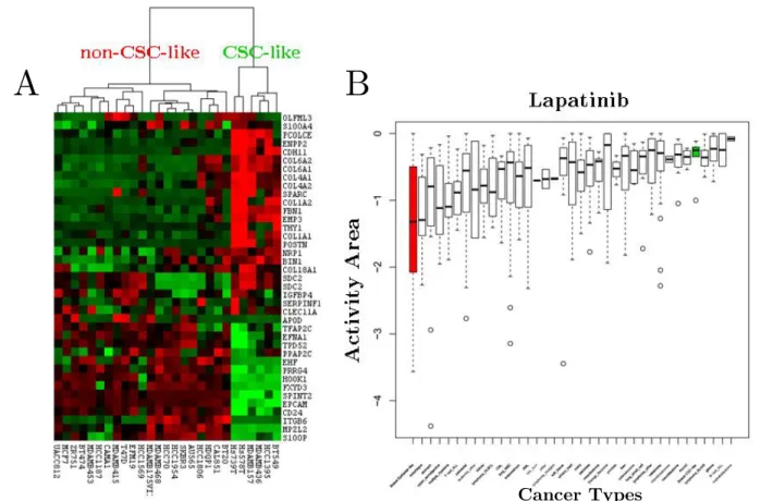
Figure 3.3: Hierarchical clustering of breast cancer cell lines in CCLE and global effectiveness distribution of Lapatinib.

(A) Hierarchical clustering of breast cancer cell lines in CCLE database identified two distinct

breast cancer clusters. The cell lines (in columns) are clustered according to Gupta et al.’s gene list (in rows). Red, green and black colors in the heat-map represent high, low and intermediate gene expression. (B) Lapatinib response distributions of all cancer types, as well as breast cancer subtypes shown in the heat-map. The distribution of activity area (CCLE specific drug response parameter) values for each cancer type is shown by boxplots. Boxplots are sorted based on mean activity area within cancer types. Green and red boxplots represent CSC-like and non-CSC-like breast cancer cell lines. Lower the activity area is, more sensitive the cell lines are.

A

B

18

3.1.2. Breast Cancer Cell Lines

Besides molecular and intrinsic subtypes, breast cancer can be sub-divided into two groups according to stemness properties. Gupta et al. [22] published a list of genes up- or down-regulated in cell populations enriched for stem-like cells. We showed in Isbilen et al. [23] that those genes identified two groups of breast cancer cell lines (Figure 3.3A) with differential drug responses. We have found out that CSC-like cells were very resistant to Lapatinib compared to non-CSC-CSC-like cells and other cancer types, although Lapatinib has been approved for the treatment of HER2- and hormone-positive breast cancers (Figure 3.3B).

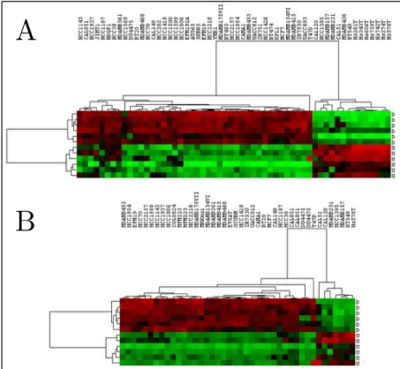
We have also developed 12-gene signature that distinguishes breast cancer cell lines according to their cancer stemness. We found the most differentially expressed genes between CSC-like and non-CSC-like breast cancer cell lines and selected 12 of them as the best classifiers. Those 12 genes separated the common cell lines in CCLE and CGP into the same clusters sharply in both databases (Figure 3.4).

Figure 3.4: Hierarchical clustering of breast cancer cell lines in CCLE (A) and CGP (B) databases based on 12-gene signature.

Red, green and black colors define high, low and intermediate expression, respectively. The genes that are up- and down-regulated in CSC-like cells were shown by U and D, respectively.

A

19 3.1.3. Colorectal Cancer Cell Lines

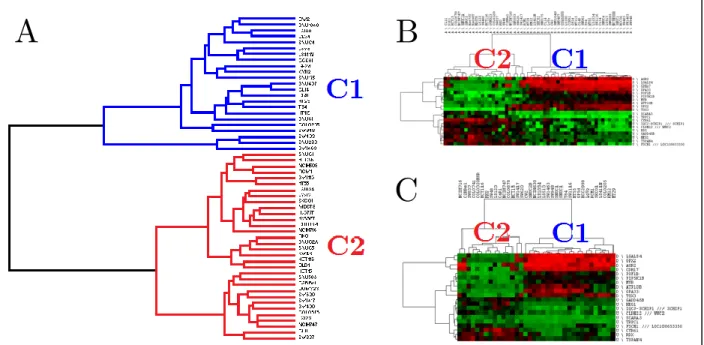
We also aimed to find out distinct subtypes of CRC cell lines with differential drug responses. We used gene expression and drug response data for the CRC cell lines from CCLE and CGP to identify gene signatures for subtypes and drug response. According to the hierarchical clustering with whole transcriptome, we identified 2 distinct clusters of CRC cell lines in CCLE database (Figure 3.5A). In order to find a gene signature that could distinguish those clusters, we found the differentially expressed genes between those clusters by t-test in CCLE database. We selected 20 out of 200 most differentially expressed genes as a gene signature for the clusters by Maximum Relevance Minimum Redundancy (MRMR) approach. Those 20-gene signature separated the same cell lines into same clusters in both CCLE and CGP databases (Figure 3.5B-C).

Figure 3.5: Hierarchical clustering of CRC cell lines in CCLE and CGP databases.

WTHC result for CRC cell lines (A) in CCLE database is shown as a dendogram. Hierarchical clustering of CRC cell lines in CCLE (B) and CGP (C) databases based on the most differentially expressed genes between clusters defined by WTHC (C1 and C2) are shown as heat-maps with dendograms. Red, green and black colors in the heat-maps represent high, low and intermediate expression, respectively.

A

B

20

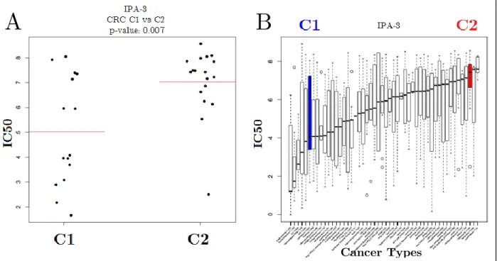
We also found some drugs for which the clusters exhibited differential drug responses. Cluster 1 cells were significantly more sensitive to IPA-3 than cluster 2 cells. Cluster 1 cells were also one of the most sensitive cell types to IPA-3 among all other cancer types, as cluster 2 cells were one of the most resistant cancer types compared to others (Figure 3.6).

This way, we developed a 20-gene signature that could identify distinct CRC cell line subtypes with differential drug response. However, it still remains to be validated in vitro.

3.2. Identification of Prognostic Subtypes in Tumors

Our next aim was to develop prognostic gene signatures in tumors using the same approach that we used for the identification of chemotherapeutic subtypes. We performed

Figure 3.6: Comparison of IPA-3 response of CRC cell line sub-groups and global effectiveness of IPA-3.

IPA-3 IC50 distributions of clusters of CRC cell lines are shown in jitter plots (A) and all cancer types in boxplots (B). Red horizontal lines in (A) represent average IC50 values for C1 and C2. Blue and red boxplots represent IPA-3 IC50 distributions C1 and C2 CRC clusters, respectively.

A

B

21

hierarchical clustering with 1000 most variant genes using GSE17536 CRC dataset, but we could not identify distinct clusters with different prognostic outcomes according to the expression of those most variant genes (data now shown), probably due to heterogeneity of tumors.

We decided to develop new algorithms that we can use to find new prognostic gene markers. In concordance with the report published by Venet et al. [24] in which they claim that most of the random signatures with high number of genes were significantly associated with clinical outcome, we decided to find single-gene markers instead of multi-gene signatures. Therefore, we decided to develop two different R-based programs, called SSAT and USAT, which analyze normalized microarray datasets with different statistical methods and 12 different algorithms using clinical data to identify prognostic single-gene markers.

We analyzed three different microarray datasets with SSAT and USAT to identify candidate prognostic gene markers in CRC. We used GSE17536, GSE17537 with SSAT and GSE17536 and GSE41258 with USAT (Table 3.1) and identified different candidate genes with each approach. We tried to validate those results with qPCR experiments of identified genes by using a unique CRC cohort (Table 3.1).

3.2.1. SSAT

SSAT is an R-based program that can analyze microarray datasets by using Log-Rank test with different expression cut-offs of genes in order to find prognostic gene markers in cancers. SSAT uses only one probeset, which has the highest coefficient of variation value, for each gene. A gene is considered as significant if its corresponding probeset is significant (p<0.05) in Log-Rank test for given expression cut-off values.

22

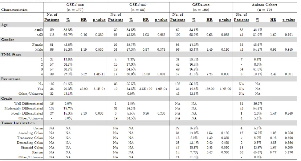
Table 3.1: Clinical Characteristics and univariate CoxPH analysis results for GSE17536, GSE17537, GSE41258 and Ankara cohort.

23

SSAT discretized the expression values for each gene as explained in Discretization of Expression Values section. We determined 8 different expression intervals for each gene. We used sequential combinations of those intervals for each gene to separate patients into high and low expression groups for Log-Rank test, e.g. ULBP2 (123) vs. ULBP2 (45678). We performed Log-Rank tests for 7 different interval cut-offs in 8 categories for each gene.

3.2.1.1. Gene Selection for Validation

We analyzed two colon cancer datasets, GSE17536 and GSE17537, for all the genes according to those interval cut-off values and identified the ones significant in both datasets. We identified 400 and 269 and 64 genes with different expression cut-offs in GSE17536, GSE17537 and common, respectively (Figure 3.7). We averaged Log-Rank

p-Figure 3.7: Schematic representation of SSAT approach.

Each green box shows a step for the selection of genes for further analysis. The number of significant genes in each step are indicated.

24

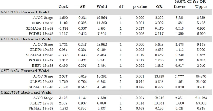
values of the genes with the same interval cut-off in both datasets and selected top 17 and 4 genes in GSE17536 and GSE17537, respectively, for multivariate logistic regression with forward and backward Wald selection method. ULBP2 and SEMA5A were the only significant independent prognostic genes in both datasets (Table 3.2). We decided to measure qPCR expression values of ULBP2 and SEMA5A in Ankara cohort for the validation of its association with prognosis.

3.2.1.2. Validation of ULBP2 and SEMA5A as Prognostic Gene Markers

Dr. Emre Dayanç with his intern students and Seçil Demirkol performed qPCR experiments for ULBP2 and SEMA5A in Ankara cohort and we analyzed the qPCR expression values with Log-Rank test and Kaplan-Meier curves in order to validate the association of ULBP2 with prognosis. We could not use SSAT to validate qPCR expression values of ULBP2 and SEMA5A, because SSAT was developed to analyze microarray expression, for which the values were normalized by GC-RMA method to be between 0 and 16, by categorizing them into 8 categories as explained in previous section.

Table 3.2: Multivariate Cox proportional Hazard regression results and corresponding statistics of selected genes in GSE17536 and GSE17537 datasets.

25

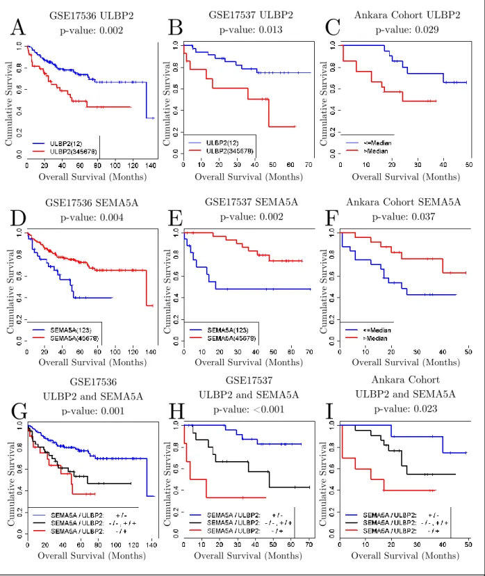
Figure 3.8: Kaplan-Meier Curves for ULBP2, SEMA5A and combination of both. Kaplan-Meier Curves for ULBP2 (A, B, C), SEMA5A (D, E, F) and combination of both (G, H, I) in GSE17536, GSE17537 and Ankara cohorts, respectively. (A, B, C, D, E, F) Blue and red colors represent low and high expression. (G, H, I) Blue, black and red colors represent good, intermediate and poor prognosis patient groups. The expression cut-off values are 4 and 6 for ULBP2 and SEMA5A, respectively, in GSE17536 and GSE17536 and median values in Ankara cohort for both genes.

A

B

C

GSE17537 ULBP2 p-value: 0.013

Ankara Cohort ULBP2 p-value: 0.029

GSE17536 SEMA5A p-value: 0.004

GSE17537 SEMA5A p-value: 0.002

Ankara Cohort SEMA5A p-value: 0.037

GSE17536 ULBP2 and SEMA5A

p-value: 0.001

GSE17537 ULBP2 and SEMA5A

p-value: <0.001

Ankara Cohort ULBP2 and SEMA5A

p-value: 0.023

D

E

F

G

H

I

Overall Survival (Months) Overall Survival (Months) Overall Survival (Months)

Overall Survival (Months) Overall Survival (Months) Overall Survival (Months)

Overall Survival (Months) Overall Survival (Months) Overall Survival (Months)

Cu m ul ativ e Su rv iv al Cu m ul ativ e Su rv iv al Cu m ul ativ e Su rv iv al Cu m ul ativ e Su rv iv al Cu m ul ativ e Su rv iv al Cu m ul ativ e Su rv iv al Cu m ul ativ e Su rv iv al Cu m ul ativ e Su rv iv al Cu m ul ativ e Su rv iv al

26

Because qPCR values were not exposed to such a normalization, we could not apply SSAT directly to qPCR values. Instead, we used median expressions as expression thresholds to separate patients into high and low expression groups and performed Log-Rank test for those separations in Ankara cohort (Figure 3.8). We identified high expression of ULBP2 and low expression of SEMA5A as significantly associated with poor prognosis in all three cohorts. We also showed that combined analysis of ULBP2 and SEMA5A further identified better poor and good prognosis groups, as well as an intermediary prognosis group, in all three cohorts (Figure 3.8).

We also performed stepwise multivariate Cox Proportional Hazard Regression analysis with backward Wald method to see whether ULBP2 and SEMA5A were prognostic classifiers independent of other clinical parameters, like age, gender, stage and grade, in Ankara cohort. The analysis results showed that ULBP2 and SEMA5A together could define good, intermediate and poor prognostic subgroups independent of other clinical parameters (Table 3.3).

3.2.1.3. Prediction of Chemotherapy Benefit with ULBP2 and SEMA5A

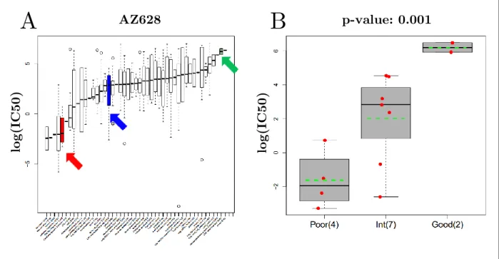
We also analyzed predictive capability of ULBP2 and SEMA5A in CRC cell lines from CGP database. We identified many drugs effective to poor prognosis sub-group of CRC cell lines determined by the combination of ULBP2 and SEMA5A gene expression. One of the drugs with the greatest differential effectiveness CRC cell lines was AZ628 (Figure 3.9). According to global effectiveness of AZ628, poor prognosis sub-group of CRC cell

Table 3.3: Stepwise multivariate Cox proportional hazard regression results and corresponding statistics of prognosis separation by ULBP2 and SEMA5A in Ankara cohort.

27

lines was one of the most sensitive cancer types to AZ628, although good prognosis subtype was almost the most resistant one among all cancer types and intermediary sub-group was somewhere in between with an average response (Figure 3.9A).

This way, we showed that ULBP2 and SEMA5A might have chemotherapy benefit prediction power, besides prognostic power. However, these findings still remain to be validated in vitro.

Figure 3.9: Global effect distribution of AZ628 (A) and differential response of prognostic CRC sub-groups to AZ628 (B).

(A)The distributions of AZ628 log(IC50) values are shown by boxplots for each cancer type. CRC cell lines were divided into three prognostic sub-groups: poor (red), intermediate (blue) and good (green) prognosis groups. (B) The distributions of AZ628 log(IC50) values of prognostic CRC sub-groups were compared with ANOVA. Each red dot represent a cell line with response to AZ628 shown in the y-axis. The distribution of the drug responses for each sub-group are shown in boxplots. Green dashed lines represent the average drug responses of sub-groups.

A

B

28 3.2.1.4. Conclusion

We identified ULBP2 and SEMA5A as independent prognostic factors in colon cancer with SSAT approach and validated their association with prognosis in an independent cohort. Moreover, we validated the independence of their association with prognosis when they were used together to assess the prognostic subgroups in colon cancer.

3.2.2. USAT

After SSAT approach, we decided to generate a more robust survival analysis tool, because SSAT was using only Log-Rank test with 7 expression cut-off values that we determined. Therefore we decided to develop an unsupervised approach with more advanced statistical methods and we call that method Unsupervised Survival Analysis Tool (USAT).

USAT uses Cox Proportional Hazard Regression (CoxPH), Maximally Selected Rank Statistics (Maxstat) and Log-Rank tests with different types of expression data and stage stratification to determine stage independent prognostic gene markers. CoxPH is used to determine hazard ratio for one unit increase in expression or between categories, Maxstat is used to determine the best expression cut-off value that can separate patients into low and high expression groups that exhibit the best prognosis difference and Log-Rank test is used to see whether the prognosis difference between high and low expression groups is significant or not. Any gene is considered as significant when any of their probesets are significant in all those three statistical tests.

Before analyzing any datasets with USAT, we performed secondary analyses to calculate true and false positivity rates in order to determine how reliable USAT’s results are. Finally, we developed different versions of USAT by generating different models to

29

improve true and false positivity rates and started analyzing different CRC datasets with the latest version.

3.2.2.1. True Positivity of USAT

The first version of USAT analyzed stage-stratified categorical expression values with CoxPH, continuous expression values with Maxstat and Log-Rank tests (CGS-MC-LC, see Model Generation in Methods section). To determine the true positivity of this approach, we used 48-gene CRC prognostic gene list published by O’Connell et al. [12] as reference. In other words, we checked how many of those 48 genes were present as significant in USAT results of the test set (GSE17536). We were able to analyze 44 of those 48 genes due to lack of probesets for 4 of the gene symbols in the HG-U133 Plus 2.0 platform. USAT validated 21 genes among those 44 genes (Table 3.4), which makes the true positivity of the first version of USAT ~48%. 48% true positivity suggested that we would not be validating half of the genes, which we found by USAT in one dataset, with another dataset. Therefore, we decided to generate different models with different combinations of statistical tests, types of expression and stage stratification to see whether we can improve USAT’s true positivity.

3.2.2.1.1. USAT with Different Models

In the first version of USAT, we were using categorical expression values and stage stratification with CoxPH, continuous expression values with Maxstat and Log-Rank tests (CGS-MC-LC). Latter, we generated 11 new models to find the best one that could find the maximum number of 48 genes published by O’Connell et al. as prognostic genes in CRC. When we analyzed the test set with 12 different models of USAT, we realized that all the models could identify similar numbers of genes. However, each model had the ability to identify different genes than the common ones in all models, because USAT was able to identify 33 of 44 genes when we considered the union of the results acquired by

30

all 12 models (Table 3.4). In other words, if we consider a gene as significant when it is significant in at least one of the models, then we are able to identify 33 of 44 genes with USAT. Therefore, we decided to use all 12 models in USAT, thus increasing the true positivity to from 48% to 75%.

3.2.2.2. False Positivity of USAT

We calculated false positivity rate of USAT by calculating the proportion of the probesets that exhibit opposite association with prognosis in common results of GSE17536 and GSE41258 CRC microarray datasets. USAT identified 3985 probesets corresponding to 3270 genes as CRC prognostic gene markers in GSE17536 dataset and 2408 probesets corresponding to 2025 genes in GSE41258 dataset (Figure 3.10). We found that 433 probesets corresponding to 366 genes were common in both datasets. 395 out of those 433 probesets have the same significant association with prognosis in both datasets, although the remaining 38 probesets have opposite associations with prognosis in each dataset. Thus, the proportion of the probesets that signify opposite associations with prognosis in the datasets is nearly 9%. In other words, the false positivity rate of USAT is 9% and we expect to invalidate almost 1 out of 10 genes that we identify by USAT.

3.2.2.3. Gene Selection for Validation

USAT identified 395 probesets corresponding to 329 genes as candidate CRC prognosis gene markers that exhibit the same association with prognosis in common results of

Table 3.4: Number of significant genes among 48 genes in USAT models.

31

GSE17536 and GSE41258 (Figure 3.10). In order to determine the genes for validation, we narrowed down the gene list according to independence of cancer stage and applied L1 penalized CoxPH regression to each dataset to find the best candidates. After selection through stage independence, we got 66 probesets corresponding to 65 genes. We applied L1 penalized CoxPH regression to those 66 probesets and identified 6 probesets corresponding to 6 genes in GSE17536 and 4 probesets corresponding to 4 genes in GSE41258 (Figure 3.10).

We selected 5 of 6 genes (DUSP10, PCSK5, TGFB1I1, PLS3 and CLCN7) from GSE17536 and 3 of 4 genes (PTRF, CLDN3 and KLF9) from GSE41258 for validation. Table 3.5 and Table 3.6 show the results of the statistical analyses used in USAT with continuous expression values for GSE17536 and GSE41258 and the results of 12 models of USAT in

Figure 3.10: Schematic representation of USAT approach.

Each blue box shows a step for the selection of genes for further analysis. The number of significant probesets and corresponding genes in each step are also indicated.

32

both datasets, respectively. USAT identified PTRF, PCSK5, TGFB1I1, DUSP10, KLF9 and PLS3 as poor prognosis markers and CLCN7 and CLDN3 as good prognosis markers in both datasets (Table 3.5 and Table 3.6). Although PTRF, PCSK5, TGFB1I1, DUSP10 and PLS3 were significant for all 12 models in only GSE17536, KLF9 is the only gene that was significant for all 12 models in both datasets and GSE41258 itself (Table 3.6). Chi-square test results also showed that there was no significant association between cancer stage and expression of those genes in both datasets (Table 3.5).

3.2.2.4. Validation of Microarray Expression with qPCR Expression

We identified candidate genes for validation in two different microarray datasets with USAT and we used qPCR to measure the expression of those candidate genes in Ankara cohort for validation. The validation of microarray expression by qPCR expression is still a controversial issue. There are many reports that emphasize the general problems on validation of microarray expression with qPCR expression, like variability in hybridization efficiency of sequences, differences in design, differences in probes and target labeling etc.

Table 3.5: Results of USAT analyses with continuous microarray expression values for GSE17536 and GSE41258.

33

even in the same cohorts [25, 26, 27, 28]. In this step, we try to validate microarray results of two cohorts with qPCR expression of another cohort. In other words, we have both different gene expression measurement techniques and different cohorts for validation. Therefore, we wanted to make sure that microarray chips and qPCR primers detect and measure the expression of the same transcripts, so that we measure the same thing in different cohorts. For that reason, we performed qPCR experiments for the selected genes using 7 different CRC cell lines whose microarray expression data was available in CGP database. We compared qPCR and microarray expression of the selected genes in those 7 cell lines and found out that the qPCR primers of 6 of 8 genes (PTRF, TGFB1I1, DUSP10, KLF9, CLCN7 and CLDN3) could validate the microarray expression of the cell lines (Figure 3.11). So, we decided to perform qPCR experiments in our cohorts with the genes whose qPCR expression validated the microarray counterparts.

3.2.2.5. Validation of USAT Results

We performed qPCR experiments in Ankara cohort for the genes whose microarray expression were validated with qPCR expression. We performed USAT analysis in Ankara cohort using qPCR expression values. Table 3.7 shows the results of USAT analysis performed with continuous qPCR expression values in Ankara cohort for the selected

Table 3.6: Results of USAT’s 12 Models for GSE17536 and GSE41258.

34

genes for validation and corresponding 12-model results. As shown in Table 3.7, the only gene whose association with prognosis could be validated by qPCR experiments was CLCN7. Surprisingly, all the other genes identified in microarrays were identified as either oppositely associated with prognosis (PTRF, TGFB1I1, DUSP10) or unrelated to prognosis at all (KLF9, CLDN3) in Ankara cohort.

3.2.2.5.1. Log-Rank Analysis with Multiple Cut-off Values (LRMC)

After we identified opposite associations with prognosis in Ankara cohort for most of the selected genes, we thought that the problem could be in the analysis of each gene with a single expression threshold value determined by Maxstat analysis. Maxstat analysis determines an expression cut-off that gives the biggest absolute log-rank statistics.

Figure 3.11: Concordance between qPCR and microarray expression of the genes selected for validation.

Each dot represents the microarray and qPCR expression of the indicated gene in the x-axis and y-axis, respectively. Red line is the best linear fit. Pearson r and corresponding p-values are indicated on top of the graphs. Green and red squares indicate concordance and discordance, respectively, between microarray and qPCR expression.

35

Analysis of each gene with a single expression cut-off may have led us to ignore other possible cut-off values that show different associations with prognosis for the same gene. Therefore, we decided to analyze all possible expression cut-off values with Log-Rank test for each gene in terms of the direction of their association with prognosis. Figure 3.12 shows a representative LRMC analysis result for PTRF in Ankara cohort. The lower graph in Figure 3.12 shows the Log-Rank p-values in the y-axis calculated for expression threshold values in the x-axis, which separate patients into high and low expression groups for Log-Rank test. Although most of the threshold values could not pass 0.05 significance level, high expression of PTRF is associated with good prognosis in almost all the threshold values, including those were significant as well. That graph suggests that whichever PTRF expression cut-off value is selected for grouping patients into high and low expression groups, high PTRF expression suggests an association with good prognosis in Ankara cohort. So, that graph gives insight into the general behavior of a gene regarding the direction of the overall association with prognosis.

We used LRMC graphs to understand general behavior of our genes in both microarray datasets and Ankara cohort (Figure 3.13). The only gene for which we identified significant expression cut-offs that exhibited associations with prognosis in both microarray datasets and Ankara cohort in the same direction was CLCN7 (green box in Figure 3.13). High CLCN7 expression was associated with good prognosis in all three cohorts, especially for the expression cut-offs just below the 1st quartile of the expression values.

36

High expressions of PTRF, TGFB1I1, DUSP10 and KLF9 (the genes in red boxes in Figure 3.13) were associated with poor prognosis in GSE17536 and GSE41258 for all significant expression cut-offs, although the high expressions of those genes were associated with good prognosis in Ankara cohort for all significant expression cut-offs. CLDN3 (in yellow box in Figure 3.13) was the only gene for which we could not find any significant expression cut-off values. Actually, we got a very similar LRMC graph in Ankara cohort with GSE41258 for CLDN3. However, neither graphs looked like the CLDN3 LRMC graph of GSE17536, for which there were many significant expression cut-offs associated with good prognosis. Nevertheless, all the expression cut-offs for CLDN3 in all three cohorts suggested an association with good prognosis despite lack of significance.

One of the most interesting points was that the LRMC graphs of microarray datasets and Ankara cohort were very similar to each other, especially for PTRF and

Figure 3.12: LRMC analysis of PTRF in Ankara cohort.

In the scatter plot, each dot represents a Log-Rank p-value in y-axis for a given expression cut-off value in x-axis, by which the samples are separated into high and low expression groups for Log-Rank analysis. Blue and red dots represent association with good and poor prognosis, respectively. Horizontal dashed line shows 0.05 p-value threshold. Vertical gray dashed lines show 1st, 2nd and 3rd quartiles from left to right, respectively. Kaplan-Meier curves for a non-significant (left) and a significant (right) Log-Rank results are shown above. Blue and red lines represent the cumulative survival as a function of overall survival for the patients who have low and high expression of the indicated gene, respectively, based on the expression cut-offs indicated in the scatter plot.

37

TGFB1I1, although they exhibited opposite associations with prognosis. PTRF LRMC graphs contained two different peaks, which were around the 3rd quartiles and 1st quartiles of the expression values, in LRMC graphs of all three cohorts. Moreover, the most significant PTRF expression cut-off values were around the 3rd quartile of the expression values in all cohorts. In TGFB1I1 LRMC graphs, the most significant expression cut-offs were between the median and the 3rd quartile of the expression values in all the cohorts. KLF9 LRMC graph also contained similar patterns in GSE41258 and Ankara cohort. The smaller KLF9 expression cut-off values suggested opposite associations (despite being insignificant) compared to the greater KLF9 expression cut-offs in both GSE41258 and Ankara cohort.

Figure 3.13: LRMC analysis of the selected genes in GSE17536, GSE41258 and Ankara cohort.

Genes and cohorts are represented in columns and rows, respectively. Each dot represents a Log-Rank p-value in y-axis for a given expression cut-off value in x-axis, by which the samples are separated into high and low expression groups for Log-Rank analysis. Blue and red dots represent association with good and poor prognosis, respectively. Horizontal black dashed lines show the 0.05 p-value threshold. Vertical gray dashed lines show 1st, 2nd (median) and 3rd quartiles from left to right, respectively. Red, green and yellow rectangles show the opposite, similar and insignificant associations with survival, respectively.