Equivalence of linear canonical transform
domains to fractional Fourier domains and the
bicanonical width product: a generalization of the
space–bandwidth product
Figen S. Oktem1,2,*and Haldun M. Ozaktas1 1Department of Electrical Engineering, Bilkent University, TR-06800 Bilkent, Ankara, Turkey 2
Currently with the Department of Electrical and Computer Engineering, University of Illinois at Urbana-Champaign, Urbana, Illinois 61801, USA
*Corresponding author: oktem1@illinois.edu
Received March 29, 2010; accepted May 25, 2010; posted June 30, 2010 (Doc. ID 126134); published July 30, 2010
Linear canonical transforms (LCTs) form a three-parameter family of integral transforms with wide applica-tion in optics. We show that LCT domains correspond to scaled fracapplica-tional Fourier domains and thus to scaled oblique axes in the space–frequency plane. This allows LCT domains to be labeled and ordered by the corre-sponding fractional order parameter and provides insight into the evolution of light through an optical system modeled by LCTs. If a set of signals is highly confined to finite intervals in two arbitrary LCT domains, the space–frequency (phase space) support is a parallelogram. The number of degrees of freedom of this set of sig-nals is given by the area of this parallelogram, which is equal to the bicanonical width product but usually smaller than the conventional space–bandwidth product. The bicanonical width product, which is a generali-zation of the space–bandwidth product, can provide a tighter measure of the actual number of degrees of free-dom, and allows us to represent and process signals with fewer samples. © 2010 Optical Society of America
OCIS codes: 050.5082, 070.0070, 070.2025, 070.2575, 070.2590, 080.2730.
1. INTRODUCTION
The conventional space–bandwidth product is of funda-mental importance in signal processing and information optics because of its interpretation as the number of de-grees of freedom of signals [1–17]. In this paper, we dis-cuss the bicanonical width product, which generalizes the space–bandwidth product and which can often provide a tighter measure of the actual number of degrees of free-dom.
The definition of the bicanonical width product is based on linear canonical transforms (LCTs), which are a three-parameter family of linear integral transforms [16,18]. The Fourier and fractional Fourier transforms (propaga-tion through quadratic graded-index media), coordinate scaling (imaging), chirp multiplication (passage through a thin lens), and chirp convolution (Fresnel propagation in free space) are some of the special cases of this family of transforms. Because concatenation of LCTs are also LCTs, the family of LCTs can model a broad class of opti-cal systems involving arbitrary combinations of any num-ber of lenses, sections of free space, and sections of graded-index media. These systems belong to the class of quadratic-phase systems, which are also known as ABCD systems or lossless first-order optical systems [18–27]. LCTs have also been referred to as generalized Huygens integrals [28], generalized Fresnel transforms [29,30], special affine Fourier transforms [31,32], extended frac-tional Fourier transforms [33], and Moshinsky–Quesne transforms [18], among other things, and have found use in image filtering [34]. In this paper we show that LCT
domains are essentially equivalent to fractional Fourier domains.
We will provide motivation, interpretation, and an overview of the main ideas and results in Section 2, which will then be substantiated in Sections 3–5. The definition and properties of LCTs will be briefly reviewed in Section 3. In Section 4 we establish the equivalence of LCT do-mains to fractional Fourier dodo-mains. The relationships between the space-frequency support, the bicanonical width product, and the number of degrees of freedom is the subject of Section 5. We conclude in Section 6. This work is based on [35].
2. OVERVIEW
A. Equivalence of Linear Canonical Transform Domains to Fractional Fourier Domains
One of the most important concepts in Fourier analysis is the concept of the frequency (or Fourier) domain. This do-main is understood to be a space where the frequency rep-resentation of the signal lives. Since the fractional Fou-rier transform (FRT) has the effect of rotating the space-frequency (phase space) representation of a signal,
fractional Fourier domains correspond to oblique axes in
the space-frequency plane (phase space) [16,36]. By anal-ogy with the concept of fractional Fourier domains, the term linear canonical domain has been used in several papers to refer to the domain of the LCT representation of a signal [37–46]. However, it has not been clear what or where these domains are. In other words, while the effect
of an LCT on the space-frequency representation of a sig-nal is well understood as a linear geometrical distortion, it has not been obvious how members of the three-parameter family of LCT domains are related to the space-frequency plane, or how we should visualize them. One of our contributions is to explicitly relate LCT do-mains to the space-frequency plane. We will show that
each LCT domain corresponds to a scaled FRT domain and thus a scaled oblique axis in the space-frequency plane [35]. Based on this many-to-one association of LCTs with FRTs, LCT domains can be labeled and monotoni-cally ordered by an associated fractional order parameter, instead of their usual three parameters, which do not di-rectly lend themselves to a natural ordering.
This has important implications for optical systems modeled by LCTs (such as those consisting of arbitrary concatenations of lenses and sections of free space). The optical amplitude distribution at any plane along the op-tical axis can be expressed as a three-parameter LCT of the input. Being able to associate a single monotonically increasing parameter with each location along the optical axis offers a vastly more transparent understanding of the evolution of the optical amplitude distribution, as op-posed to imagining that the light goes through an uniden-tified and unsequenced series of three-parameter domains whose whereabouts we cannot visualize. This interpreta-tion of LCT domains also ties together the LCT descrip-tion of such optical systems with descripdescrip-tions viewing propagation as an act of continual fractional Fourier transformation [47,48].
The association between LCT and FRT domains is based on expressing the LCT as a chirp multiplied and scaled FRT, which is a special case of the widely known Iwasawa decomposition [24,25,49]. Multiplication with a function is not usually considered to be an operation that changes the domain of a signal, and scaling of the axis is a relatively trivial modification of a domain. Therefore, LCTs of a signal that are associated with the same FRT order parameter essentially live in the same domain (the FRT domain with that order). We will speak of LCT do-mains sharing the same order parameter as essentially equivalent domains. If a signal is confined to a finite in-terval in a certain LCT domain, it will also be confined to a finite interval in all essentially equivalent domains. B. Generalization of the Space–Bandwidth Product: The Bicanonical Width Product
1. Space–Bandwidth Product
Let us first recall the construction of the concept of the conventional space–bandwidth product. Consider a family of signals whose members are approximately confined to an interval of length⌬u in the space domain and to an interval of length ⌬ in the frequency domain in the sense that a large percentage of the signal energy is con-fined to these intervals. The space–bandwidth product N is defined [12,16] as
N⬅ ⌬u⌬, 共1兲
and is always greater than or equal to unity because of the uncertainty relation.
The conventional space–bandwidth product is the mini-mum number of samples required to uniquely identify a signal out of all possible signals whose energies are ap-proximately confined to space and frequency intervals of length ⌬u and ⌬. This argument is based on the Shannon–Nyquist sampling theorem, which requires that the spacing between samples not be greater than ␦u
= 1 /⌬, so that the minimum number of samples over the extent ⌬u is given by ⌬u/␦u =⌬u⌬. Alternatively, if we
sample the signal in the frequency domain, the spacing between samples should not be greater than␦=1/⌬u, so that the minimum number of samples over the extent⌬ is given by ⌬/␦=⌬u⌬. The minimum number of samples needed to fully characterize an approximately space- and band-limited signal can also be interpreted as the number of degrees of freedom of the set of signals. This number of samples turns out to be the same whether counted in the space or frequency domain, and is given by the space–bandwidth product.
When the approximate space and frequency extents are specified as above, this amounts to assuming that most of the energy of the signal is confined to a⌬u⫻⌬ rectan-gular region in the space–frequency plane, perpendicular to the space–frequency axes (Fig. 1). In this case, the number of degrees of freedom and the space–bandwidth product are both equal to the area of this rectangular re-gion. More generally, the number of degrees of freedom is given by the area of the space–frequency support (phase space support), regardless of its shape [14,16]. (The space–frequency support can be roughly defined as the re-gion in the space–frequency plane in which a large per-centage of the total energy is confined.) When the space– frequency support is not a rectangle perpendicular to the axes, the actual number of degrees of freedom will be smaller than the space–bandwidth product of the signal [14,16].
The space–bandwidth product is a notion originating from the simultaneous specification of the space and fre-quency extents. Although this product is commonly seen as an intrinsic property, it is in fact a notion that is spe-cific to the Fourier transform and the frequency domain. It is also possible to specify the extents in other FRT or LCT domains. The set of signals thus specified will in gen-eral exhibit a nonrectangular space–frequency support. We will show that when two such extents are specified, the support will be a parallelogram. In all cases, the area of the support will correspond to the number of degrees of freedom of the set of signals thus defined. If we insist on characterizing this set of signals with conventional space
µ
u
∆µ
∆u
Fig. 1. Rectangular space–frequency support with area equal to the space–bandwidth product⌬u⌬.
and frequency extents, the space–bandwidth product will overstate the number of degrees of freedom.
Obviously, specifying a finite extent in a single LCT do-main does not define a family of signals with a finite num-ber of degrees of freedom, just as specifying a finite extent in only one of the conventional space or frequency do-mains does not. However, specifying finite extents in two distinct LCT domains allows us to define a family of sig-nals with a finite number of degrees of freedom. The num-ber of degrees of freedom will depend on both the specified LCT domains and the extents in those domains.
2. Bicanonical Width Product
We now define the space–canonical width product, which gives the number of degrees of freedom of signals that are approximately confined to a finite interval⌬u in the con-ventional space domain and to a finite interval ⌬uT in some other LCT domain [35,50]:
N⬅ ⌬u⌬uT兩兩. 共2兲
This is always greater than or equal to unity because of the uncertainty relation for LCTs [16,18,40,45]. Here T represents the three parameters of the LCT, which will be explicitly defined in Section 3. Here, which can assume any real value, is one of the three parameters of the LCT in question. The space–canonical width product consti-tutes a generalization of the space–bandwidth product, and reduces to it when the LCT reduces to an ordinary Fourier transform, upon which ⌬uT reduces to ⌬ and =1.
In the above, one of the two domains was chosen to be the conventional space domain. More generally, the two LCT domains can both be arbitrarily chosen. In this case, we use the more general term bicanonical width product to refer to the product [35,50]
N⬅ ⌬uT1⌬uT2兩1,2兩, 共3兲
where⌬uT1and⌬uT2are the extents of the signal in two arbitrary LCT domains and1,2is the parameter of the
LCT between these two domains (the LCT that trans-forms the signal from the first LCT domain to the second). If=⬁ in Eq.(2)or1,2=⬁ in Eq.(3), then the product N
will not be finite, and the number of degrees of freedom will not be finite. We shall see in Section 3 that when this parameter is infinity, the two domains are related to each other simply by a scaling or chirp multiplication opera-tion. But as discussed before, domains related by such op-erations are essentially equivalent. Thus, specification of the extent in two such domains does not constrain the family of signals more than the specification of the extent in only one domain, which, as noted, is not sufficient to make the number of degrees of freedom finite.
The space–canonical width product is the minimum number of samples required to uniquely identify a signal out of all possible signals whose energies are approxi-mately confined to a space interval of⌬u and a particular LCT interval of⌬uT. This number of samples can be used to reconstruct the signal. This can be justified by the use of the LCT sampling theorem [38,51,52], which is a gen-eralization of the FRT sampling theorem [53–58]. Accord-ing to the LCT samplAccord-ing theorem, the space-domain
sam-pling interval for a signal that has finite extent⌬uTin a particular LCT domain should not be larger than ␦u
= 1 /共兩兩⌬uT兲. If we sample the space-domain signal at this rate, the total number of samples over the extent⌬u will be given by⌬u/␦u =⌬u⌬uT兩兩, which is precisely equal to the space–canonical width product. Alternatively, if we sample in the LCT domain, the sampling interval should not be larger than␦uT= 1 /共兩兩⌬u兲. Sampling at this rate, the total number of samples over the extent⌬uTis given by ⌬uT/␦uT=⌬u⌬uT兩兩, which once again is the space– canonical width product.
The derivation above can be easily replicated for the more general bicanonical width product defined in Eq.(3). Therefore, the bicanonical width product can also be
in-terpreted as the minimum number of samples required to uniquely identify a signal out of all possible signals whose energies are approximately confined to finite intervals in the two specified LCT domains, and therefore as the num-ber of degrees of freedom of this set of signals.
3. Space–Frequency Support and Degrees of Freedom
Finite extent constraints in the space and frequency do-main are well-known to translate to vertical and horizon-tal corridor constraints in the space–frequency plane. (With the term “corridor” we are referring to an infinite strip in the space–frequency plane perpendicular to a par-ticular domain.) This result can be precisely stated in terms of the Wigner distribution, one of the most fre-quently used space–frequency representations in optics [59–63]. It is not difficult to extend this result to FRT do-main constraints, which translate to oblique corridor con-straints in the space–frequency plane. However, without the equivalence of LCT domains to scaled FRT domains that we present, the effect of LCT domain constraints in the space–frequency plane has not been clear. With this equivalence, it becomes possible to see that LCT domain constraints also translate to oblique corridor constraints. Therefore, restricting the signal to finite intervals in two
distinct LCT domains implies that the space–frequency support is a parallelogram (see Fig.2below); moreover, the area of the parallelogram is equal to the bicanonical width product [35]. (Indeed, the bicanonical width product can be interpreted as a formula for the area of the parallelo-gram.) This provides further justification for interpreting the bicanonical width product as the number of degrees of freedom of LCT-limited signals.
µ
u
u
a1u
a2 ∆uT1 M1 ∆uT2 M2Fig. 2. Space–frequency support when finite extents are speci-fied in two LCT domains. The area of the parallelogram is equal to⌬uT
4. Efficient Signal Representation
There is no reason to think that families of signals en-countered in practice will necessarily uniformly fall into a rectangular region in the ordinary space–frequency plane. As well understood, when the family of signals does not have a rectangular space–frequency support perpen-dicular to the space–frequency axes, the space–bandwidth product overstates the actual number of degrees of free-dom. That is, we can represent these signals with a num-ber of samples less than the space–bandwidth product. In some applications, where the underlying physics involves LCT type integrals (as is the case with many wave propa-gation problems and optical systems), parallelograms may be excellently, if not perfectly, tailored to the true space–frequency supports.
Even when this is not the case, it may frequently be possible to more tightly enclose the actual space– frequency support with a parallelogram than with a angle perpendicular to the axes, or indeed with any rect-angle. Then, the bicanonical width product may better represent the actual number of degrees of freedom, and we will be able to represent the signals with fewer samples [35].
Even when confronted with a space–frequency support of arbitrary shape, it is quite common to assume the num-ber of degrees of freedom to be equal to the space– bandwidth product and work with that many samples, without regard to the shape of the space–frequency sup-port. In reality, this is an inefficient worst-case approach, which encloses the arbitrary shape within a rectangle perpendicular to the axes, and thus which overstates the number of degrees of freedom. Why is this approach so common? Because in general there is no easy and general way of handling arbitrary irregular space–frequency sup-ports. There is no guarantee that such signals can be rep-resented with space domain or other linear unitary trans-form domain samples with the number of samples being equal to the number of degrees of freedom. In general, it is necessary to find a custom basis in which the signals can be represented with a number of coefficients equal to the number of degrees of freedom, and it may not always be easy to find such a convenient basis.
While our approach does not fully solve this problem, it offers a general approach allowing the representation and processing of signals with a number of samples closer to their true number of degrees of freedom. Having the
free-dom to enclose a given region with an arbitrary parallelo-gram is much more flexible than being restricted to enclos-ing the region with a rectangle perpendicular to the axes, or indeed with any rectangle, and in general will allow a smaller area and number of samples to be achieved [35]. Once a parallelogram minimally enclosing the true space–frequency support is found (which gives us two LCT domains in which the signals are confined to the ex-tents⌬uT1and⌬uT2), the signal can be represented with ⌬uT1⌬uT2兩1,2兩 uniform samples in these LCT domains.
Therefore, the problem of finding the smallest number of samples required to represent signals with an arbitrary space–frequency support reduces to a simple geometrical problem [35]. We simply need to find the smallest paral-lelogram enclosing the space–frequency support. Then the area of the parallelogram, which is equal to the
bica-nonical width product, will give us the minimum number of samples required to represent the signal using the LCT sampling theorem. The continuous signals can be recov-ered using the LCT interpolation formula [44,46].
5. Relation to the Discrete LCT
It is worth tying our development to a recent result [50] that showed that if the number of samples N is chosen to
be at least equal to the bicanonical width product, the dis-crete LCT (DLCT) can be used to obtain a good approxi-mation to the continuous LCT, limited only by the
funda-mental fact that a signal cannot have strictly finite extent in more than one domain [50,64]. The exact relation be-tween the discrete and continuous LCT derived in [50] precisely shows the approximation involved and demon-strates how the approximation improves with increasing
N.
Because this exact relation generalizes the correspond-ing relation for Fourier transforms [65], the DLCT de-fined in [66] and discussed in [50,64,67,68] approximates the continuous LCT in the same sense that the DFT ap-proximates the continuous Fourier transform. This el-egant and natural formulation of discrete LCT computa-tion mirrors several of the concepts we have been discussing. Rather than assuming that the space and fre-quency extents of the signals are specified in the conven-tional manner and determining the number of samples from the standard Nyquist–Shannon sampling theorem as in [69–75], in this formulation the extents are specified in the input and output LCT domains, and the number of samples are determined from the LCT sampling theorem [50]. The minimum number of samples required for com-putation is given by the bicanonical width product and the DLCT defined in [66] works with this number of samples without requiring any interpolation or oversam-pling. On the other hand, sampling the input and output conventionally as in the above cited papers usually leads to a greater number of samples and sometimes requires different numbers of samples for the input and output sig-nals. Finally we note that the DLCT in [50,64,66–68] can be efficiently computed inO共N log N兲 time by successively performing a chirp multiplication, a fast Fourier trans-form (FFT), and a second chirp multiplication [50,56,66] in a straightforward manner without the need for sophis-ticated algorithms or space–frequency support tracking.
Fast computation, a well-defined relationship to the continuous LCT, and unitarity make this definition of the DLCT an important candidate for being a widely accepted definition of the discrete version of the LCT.
3. LINEAR CANONICAL TRANSFORMS
Optical systems involving thin lenses, sections of free space in the Fresnel approximation, sections of quadratic graded-index media, and arbitrary combinations of any number of these are referred to as first-order optical sys-tems or quadratic-phase syssys-tems. Mathematically, such systems can be modeled as linear canonical transforms (LCTs). The output light field fT共u兲 of a quadratic-phase system is related to its input field f共u兲 through [16,18]fT共u兲 ⬅ 共CTf兲共u兲 ⬅
冕
−⬁ ⬁
CT共u,u⬘兲f共u⬘兲du⬘,
CT共u,u⬘兲 ⬅
冑
1 B e −i/4ei冉
D Bu 2−21 Buu⬘+ A Bu⬘ 2冊
, 共4兲for B⫽0, where CT is the unitary LCT operator with pa-rameter matrix T =关A B;C D兴 with AD−BC=1. In the trivial case B = 0, the LCT is defined simply as fT共u兲 ⬅
冑
Dexp关iCDu2兴f共Du兲. Sometimes the three realparam-eters ␣=D/B, =1/B, ␥=A/B are used instead of the unit-determinant matrix T whose elements are A, B, C,
D. (One of the four matrix parameters is redundant
be-cause of the unit-determinant condition). These two sets of parameters are equivalent, and either set of param-eters can be obtained from the other [16,18]:
T =
冋
A BC D
册
=冋
␥/ 1/
− + ␣␥/ ␣/
册
. 共5兲 The transform matrix T is useful in the analysis of optical systems because if several systems are cascaded, the overall system matrix can be found by multiplying the corresponding matrices.The LCT family includes the Fourier and fractional Fourier transforms, coordinate scaling, and chirp multi-plication and convolution operations as its special cases.
The ath-order fractional Fourier transform (FRT) [16] of a function f共u兲, denoted by fa共u兲, is most commonly de-fined as
fa共u兲 ⬅ 共Faf兲共u兲 ⬅
冕
−⬁⬁
Ka共u,u⬘兲f共u⬘兲du⬘,
Ka共u,u⬘兲 ⬅ Aei共cot u
2−2csc uu⬘+cot u⬘2兲
,
A=
冑
1 − i cot, = a/2 共6兲 when a⫽2j, Ka共u,u⬘
兲=␦共u−u⬘
兲 when a=4j, and Ka共u,u⬘
兲=␦共u+u⬘
兲 when a=4j±2, where j is an integer. The FRT is a special case of the LCT with matrixFa=
冋
cos sin − sin cos
册
, 共7兲differing only by an inconsequential factor: CFaf共u兲
= e−ia/4Faf共u兲 [16,18].
Another special case of the LCT is multiplication with a chirp function of the form exp关−iqu2兴, which corresponds
to a thin lens in optics. The corresponding LCT matrix is given by
Qq=
冋
1 0
− q 1
册
. 共8兲Propagation through a section of free space in the Fresnel approximation is equivalent to convolution with a chirp function of the form e−i/4
冑
1 / rexp关iu2/ r兴. Thecor-responding LCT matrix is given by Rr=
冋
1 r
0 1
册
. 共9兲Optical imaging can be modeled as a scaling operation, which maps a function f共u兲 into
冑
1 / Mf共u/M兲 with M⬎0. The transformation matrix isMM=
冋
M 0
0 1/M
册
. 共10兲An arbitrary LCT can be decomposed into a FRT fol-lowed by scaling folfol-lowed by chirp multiplication [16,71]:
T =
冋
A B C D册
=冋
1 0 − q 1册
冤
M 0 0 1 M冥
冋
cos sin − sin cos 册
. 共11兲 Here, q is the chirp multiplication parameter, M⬎0 is the scaling factor, and =a/2, where a is the order of the FRT. The decomposition can be written more explicitly in terms of the LCT and FRT domain representations of the signal asfT共u兲 = exp关− iqu2兴
冑
1Mfa
冉
uM
冊
. 共12兲This decomposition is a special case of the Iwasawa de-composition [24,25,49]. (For a discussion of the implica-tions of this decomposition to the propagation of light through first-order optical systems, see [47].) As we will see, by appropriately choosing the three parameters a, M,
q, the above equality can be satisfied for any ABCD
ma-trix. Solving for a, M, q in Eq.(11), we obtain the decom-position parameters in terms of the matrix entries A, B,
C, D: a =
冦
2 arctan冉
B A冊
, if A艌 0 2 arctan冉
B A冊
+ 2, if A⬍ 0冧
, 共13兲 M =冑
A2+ B2, 共14兲 q =冦
−C A− B/A A2+ B2, if A⫽ 0 −D B, if A = 0冧
. 共15兲The range of the arccotangent lies in共−/2,/2兴. The Wigner distribution (WD) of a signal Wf共u,兲 is a phase-space distribution that gives the distribution of sig-nal energy over space and frequency, and is defined as [16,76]
Wf共u,兲 =
冕
−⬁⬁
f共u + u⬘/2兲f*共u − u⬘/2兲e−i2u⬘du⬘. 共16兲
The WD of fT共u兲 can be related to the WD of f共u兲 by a lin-ear distortion [16]:
WfT共u,兲 = Wf共Du − B,− Cu + A兲. 共17兲
The Jacobian of this coordinate transformation is equal to the determinant of the matrix T, which is unity. There-fore, this coordinate transformation will geometrically distort the support region of the WD, but the support area will remain unchanged.
4. RELATION BETWEEN FRACTIONAL
FOURIER DOMAINS AND LINEAR
CANONICAL DOMAINS
As is well-known, fractional Fourier domains correspond to oblique axes in the space–frequency plane [36]. The ef-fect of ath-order fractional Fourier transformation on the Wigner distribution of a signal is to rotate the Wigner dis-tribution by an angle=a/2 [36,77,78]:
Wfa共u,兲 = Wf共u cos − sin ,u sin + cos 兲.
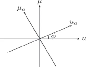
共18兲 The Radon transform operatorRDN, which takes the in-tegral projection of the Wigner distribution of f共u兲 onto an axis making an angle with the u axis, can be used to restate this property in the following manner [16]:
兵RDN关Wf共u,兲兴其共ua兲 = 兩fa共ua兲兩2, 共19兲 where uadenotes the axis making angle=a/2 with the u axis. That is, projection of the Wigner distribution of f共u兲 onto the uaaxis gives兩fa共ua兲兩2, the squared magnitude of the ath-order FRT of the function. Hence, the projec-tion axis uacan be referred to as the ath-order fractional Fourier domain (see Fig. 3) [36,77]. The space and fre-quency domains are merely special cases of the con-tinuum of fractional Fourier domains.
Recently, there has been considerable interest in gener-alizing the fractional Fourier transform and its properties to linear canonical transforms. In analogy with fractional Fourier domains, the term LCT domain has been used to refer to the domain of the LCT representation of a signal [37–40,44,45,79]. However, unlike fractional Fourier do-mains, which are recognized as oblique axes in the space– frequency plane [16,18,36], it has not been well under-stood where these LCT domains exist and how they are related to the space–frequency plane. Moreover, LCT do-mains are characterized by three independent param-eters. Therefore, LCT domains populate a three-parameter space, which makes them hard to visualize.
We first introduce the concept of essentially equivalent
domains by using the Iwasawa decomposition. As given in
Eq.(12), any arbitrary LCT can be expressed as a chirp multiplied and scaled FRT. Thus, in order to compute the LCT of a signal, we can first compute the ath-order FRT of the signal, which transforms the signal to the ath-order fractional Fourier domain. Second, we scale the trans-formed signal. Because scaling is a relatively trivial op-eration, we need not interpret it as changing the domain of the signal, but merely a scaling of the coordinate axis in the same domain. Finally, we multiply the resulting sig-nal with a chirp to obtain the LCT. Multiplication with a function is not considered an operation that transforms a signal to another domain, but one that alters the signal in the same domain. (For instance, when we multiply the Fourier transform of a function with a mask, the result is considered to remain in the frequency domain.) Therefore, only the FRT part of the LCT operation corresponds to a genuine domain change, and the linear canonical trans-formed signal essentially lives in a scaled fractional Fou-rier domain. In other words, LCT domains are essentially
equivalent to scaled fractional Fourier domains. Despite
their three parameters, LCT domains do not constitute a richer family of domains than FRT domains. More explic-itly:
In the space–frequency plane, the LCT domain with pa-rameter matrix关A B;C D兴 corresponds to a scaled oblique axis making angle arctan共B/A兲 with the u axis (or equiva-lently having slope B / A) and with scale parameter M =
冑
A2+ B2.Note that any LCT domain is completely characterized by the two parameters A and B (or equivalently by a and
M, or by␥ and ) instead of all three of its parameters.
Observe that LCTs with the same value of B / A (or equivalently the same value of ␥) will have the same value of a in the decomposition in Eq.(13), and therefore will be associated with the same FRT domain. We refer to such LCT domains, as well as their associated FRT do-main, as essentially equivalent domains. Note that if a signal has a compact support in a certain LCT domain, then the signal will also have compact support in all es-sentially equivalent domains.
The concept of essentially equivalent domains we intro-duce allows many earlier observations and results to be seen in a new light, making them almost obvious or more transparent. For instance, it has been stated that if a par-ticular LCT of a signal is band limited, then another LCT of the signal cannot be band limited unless B1/ A1
= B2/ A2 [40]. Since we recognize the domains associated
with two LCTs satisfying this relation to be essentially equivalent, this result becomes obvious. Although we will not further elaborate, other results regarding the compactness/band limitedness of different LCTs of a sig-nal [80] can be likewise easily understood in terms of the concept of essentially equivalent domains. As a final ex-ample, we consider the LCT sampling theorem [38,51,52], according to which if the LCT of a signal has finite extent ⌬uT, then we should sample it with spacing ⌬u 艋兩B兩 /⌬uT. Such a sampling scheme collapses when B = 0. It is easy to understand why if we note that B = 0 implies that the LCT domain in question is essentially equivalent to the a = 0th FRT domain; that is, the domain in which
µ
u ua
µa
φ
the signal is specified to have finite extent is essentially equivalent to the domain in which we are attempting to sample the signal.
Let us now optically interpret the equivalence of LCT domains to FRT domains. Consider a signal that passes through an arbitrary quadratic-phase system. Since the light field at any plane within the system is related to the input field through an LCT, the signal will incrementally be transformed through different LCT domains. Because the three parameters of the consequential LCT domains are not sequenced, it is not easy to give any interpretation or visualize the nature of the transformation of the optical field. However, if we think of the LCT domains as being equivalent to scaled FRT domains, it becomes possible to interpret every location along the propagation axis as a FRT domain of specific order. Moreover, it has been shown that if we take the fractional order a to be equal to zero at the input of the system, then a monotonically increases as a function of the distance along the optical axis [47,48]. In other words, propagation through a quadratic-phase sys-tem can be understood as passage through a continuum of scaled FRT domains of monotonically increasing order, in-stead of passage through an unsequenced plethora of LCT domains.
(To see that the FRT parameter a is monotonically in-creasing along the z axis, observe from Eq. (13) that a ⬀arctan共B/A兲, so that a increases with B/A. Passage through a lens involves multiplication with the matrix given in Eq. (8), which does not change B / A. Passage through an incremental section of free space involves multiplication with the matrix given in Eq.(9), which al-ways results in a positive increment in a. This is because
r is proportional to the distance of propagation, and the
derivative of the new value of B / A with respect to r is al-ways positive, which implies that B / A alal-ways increases with r. A similar argument is possible for quadratic graded-index media. A more precise development may be found in [47,48].)
The distribution of light is continually fractional Fou-rier transformed through fractional domains of increasing order, which we know are oblique axes in the space– frequency plane. This understanding of quadratic-phase systems yields much more insight into the nature of how light is transformed as it propagates through such a sys-tem, as opposed to thinking of it in terms of going through a series of unsequenced LCT domains whose whereabouts we cannot visualize.
As a final remark, we note that the relation in Eq.(19) can be rewritten for the LCT of a signal as
1
M兵RDN关Wf共u,兲兴其
冉
uTM
冊
=兩fT共uT兲兩2, 共20兲
by using Eqs. (19) and (12), where uT denotes the axis making angle=arctan共B/A兲 with the u axis and scaled by M. This is another way of interpreting scaled oblique axes in the space–frequency plane as the LCT domain with parameter T.
5. SPACE–FREQUENCY SUPPORT AND
DEGREES OF FREEDOM
Having established the relationship of LCT domains to the space–frequency plane, we can now investigate the
space–frequency support of the set of signals whose ex-tents are approximately limited in two LCT domains.
Let us consider a set of signals whose members are ap-proximately confined to the intervals 关−⌬uT1/ 2 ,⌬uT1/ 2兴 and关−⌬uT2/ 2 ,⌬uT2/ 2兴 in two given LCT domains, uT1and
uT2. We want to investigate the space–frequency support of this set of signals. Since LCT domains are equivalent to scaled fractional Fourier domains, each finite interval in an LCT domain will correspond to a scaled interval in the equivalent FRT domain. To see this explicitly, we again refer to Eq.(12), which implies that if fT共u兲 is confined to an interval of length⌬uT, so is fa共u/M兲. Therefore, the ex-tent of fa共u兲 in the equivalent ath-order FRT domain is ⌬uT/ M. Thus, the set of signals in question is approxi-mately limited to an extent of⌬uT1/ M1 in the a1th-order
FRT domain, and an extent of⌬uT2/ M2in the a2th-order
FRT domain, where a1, a2 and M1, M2are related to T1,
T2through Eqs.(13)and(14).
It is well known that if the space-, frequency-, or FRT-domain representation of a signal is identically zero (or negligible) outside a certain interval, so is its Wigner dis-tribution [16,59]. As a direct consequence of this fact, the Wigner distribution of our set of signals is confined to cor-ridors of width⌬uT1/ M1and⌬uT2/ M2in the directions
or-thogonal to ua1and ua2, respectively. (With the term “cor-ridor” we are referring to an infinite strip in the space– frequency plane perpendicular to the ua axis.) The parallelogram defined by the intersection of these two cor-ridors gives us the space–frequency support of the signals (see Fig.2). The area of the parallelogram is equal to the bicanonical width product of the set of signals in question. This result will be stated as a theorem.
Theorem 1. Consider a set of signals whose members
are approximately confined to finite extents⌬uT1and⌬uT2
in the two LCT domains uT1and uT2, respectively. Let1,2 denote the parameter of the LCT that transforms signals from the first LCT domain to the second. Then, the area of the space–frequency support of these signals, which is given by a parallelogram defined by these extents (Fig.2), is equal to the bicanonical width product⌬uT1⌬uT2兩1,2兩 of the set of signals.
Proof. The two heights of the parallelogram defined by
the extents⌬uT1and⌬uT2are⌬uT1/ M1and⌬uT2/ M2,
cor-responding to the widths of the corridors. Moreover, the angle between the corridors is 2−1. Then, the area of
the parallelogram is Area = ⌬uT1 M1 ⌬uT2 M2 兩csc共2−1兲兩 共21兲 = ⌬uT1⌬uT2
M1M2兩sin2cos1− cos2sin1兩
共22兲 = ⌬uT1⌬uT2 兩A1B2− B1A2兩 共23兲 =⌬uT1⌬uT2 兩12兩 兩␥1−␥2兩 共24兲
=⌬uT1⌬uT2兩1,2兩, 共25兲
where the third and fourth equalities follow from Eqs. (11)and(5), respectively. The final result can be obtained from the matrix corresponding to the LCT operation be-tween these two domains, which is given by T2T1
−1.
䊐 Since the number of degrees of freedom of a set of sig-nals is given by the area of their space–frequency support, the theorem provides further justification for interpreting the bicanonical width product as the number of degrees of freedom of LCT-limited signals.
Let us now for a moment focus on the space–canonical width product; we assume a finite extent has been speci-fied in the space domain and in some other LCT domain. The corresponding space–frequency support is shown in Fig.4(left). If we transform to precisely the same LCT do-main in which the extent has been specified, the new space–frequency support becomes as shown in Fig. 4 (right). Here M and M
⬘
are the scaling parameters asso-ciated with the LCT and inverse LCT operations, respec-tively. Note that in both parts of the figure, the support is bounded by a vertical corridor, perpendicular to the space domain in the left part and to the LCT domain in the right. We are not surprised that the transformed support is again a parallelogram, since the linear geometric dis-tortion imparted by an LCT always maps a parallelogram to another parallelogram. Moreover, the areas of both par-allelograms are equal to each other and given by the bi-canonical width product⌬u⌬uT兩兩, so that the number of degrees of freedom also remains the same after the LCT. This does not surprise us either, since LCTs are known not to change the support area in phase space. We may summarize by stating that the bicanonical width productis a measure for the number of degrees of freedom of sig-nals that is invariant under linear canonical transforma-tion [35]. The fact that LCTs model an important family of optical systems makes the bicanonical width product a suitable invariant measure for the number of degrees of freedom of optical signals.
On the other hand, the space–bandwidth product, which is the area of the smallest bounding perpendicular rectangle, may change significantly after linear canonical transformation and quadratic-phase optical systems. (This is the reason the number of samples must be in-creased at some intermediate stages of certain previously proposed FRT and LCT algorithms that rely on the
space–bandwidth product either as the measure of the number of degrees of freedom or as the minimum number of samples required [69–75]. In contrast, fast computation of LCTs based on the results presented in [50] allows us to work with the same number of samples in both domains without requiring any oversampling. This number of samples is the minimum possible for both domains, and is given by the bicanonical width product.) This factor makes the conventional space–bandwidth product unde-sirable as a measure of the number of degrees of freedom, which we expect to be an intrinsic and conserved quantity under invertible unitary transformations.
The so-called generalized space–bandwidth product, which essentially removes the requirement that the rect-angular support be perpendicular to the axes, has been proposed [81] as an improvement over the conventional space–bandwidth product. It has been noted that this en-tity is invariant under the FRT operation (rotational in-variance), but it was emphasized that “further research is required in obtaining other forms of generalized space– bandwidth products that are invariant under more gen-eral area preserving time-frequency operations: the sym-plectic transforms” ([81], pp. 1238–1239 ). The bicanonical width product meets precisely this demand and allows us to compute LCTs with the minimum possible number of samples without requiring any interpolation or oversam-pling [50].
6. CONCLUSION
We showed that LCT domains correspond to scaled frac-tional Fourier transform (FRT) domains, and thus to scaled oblique axes in the space–frequency plane (phase space). Based on a many-to-one association of LCTs with FRTs, LCT domains can be labeled and monotonically or-dered by the corresponding fractional order parameter in-stead of their usual three parameters, which do not di-rectly lend themselves to a natural ordering. Despite their three parameters, LCT domains do not constitute a truly richer family of domains than FRT domains. LCTs of a signal that are associated with the same FRT order parameter essentially live in the same domain (the FRT domain with that order). We have referred to such LCT domains as essentially equivalent domains. If a signal is confined to a finite interval in a certain LCT domain, it will also be confined to a finite interval in all essentially equivalent domains.
An optical system consisting of arbitrary combinations of lenses, sections of free space, and quadratic graded-index media can be modeled as an LCT. The distribution of light at any plane perpendicular to the optical axis is given by an LCT of the input distribution. The equiva-lence of LCT domains to scaled FRT domains implies that the evolution of light through LCTs with different param-eters can also be interpreted as an evolution through scaled FRT domains of monotonically increasing order. This offers a more transparent view of the propagation of light through the system, as opposed to imagining that the light goes through an unsequenced series of three-parameter domains whose whereabouts we cannot visual-ize.
Fig. 4. Space-frequency support of f共u兲 (left) and fT共u兲 (right) for
space- and LCT-limited signals. The area of both parallelograms is equal to⌬u⌬uT兩兩.
The significance of the bicanonical width product, which is a generalization of the space–bandwidth product, can be established in a number of different ways. We used the LCT sampling theorem to conclude that the bicanoni-cal width product is the minimum number of samples to uniquely identify a signal out of all possible signals whose energies are approximately confined to finite intervals in two given LCT domains. The bicanonical width product gives the number of degrees of freedom of this set of sig-nals, and this number of samples can be used to recon-struct the signal by using the LCT sampling theorem.
Another line of development involves the equivalence between LCT and FRT domains. If one conventionally specifies the space-domain and frequency-domain extents for a set of signals, the space–frequency support becomes a rectangular region (Fig.1). The space–bandwidth prod-uct is equal to the area of the rectangle. By using the fact that LCT domains correspond to scaled oblique axes in the space–frequency plane, we showed that when the ex-tents are specified in two LCT domains, the space– frequency support becomes a parallelogram defined by the intersection of two oblique corridors (Fig.5). The bi-canonical width product is equal to the area of the paral-lelogram.
When confronted with a space–frequency support of ar-bitrary shape, it is quite common to assume the number of degrees of freedom to be equal to the space–bandwidth product, without regard to the shape of its space– frequency support. In reality, this is a worst-case ap-proach that encloses the arbitrary shape within a rect-angle perpendicular to the axes and overstates the number of degrees of freedom (see Fig.5).
The bicanonical width product provides a tighter mea-sure of the number of degrees of freedom than the conven-tional space–bandwidth product and allows us to repre-sent and process the signals with a smaller number of samples, since it is possible to enclose the true space– frequency support more tightly with a parallelogram of our choice, as compared with a rectangle perpendicular to the axes, or indeed any rectangle. In some applications, where the underlying physics involves LCT type integrals (as is the case with many wave propagation problems and optical systems), parallelograms may be excellently, if not perfectly, tailored to the true space–frequency supports of the signals.
Another important feature of the bicanonical width product is that it is invariant under linear canonical
transformation. The fact that LCTs model an important family of optical systems makes the bicanonical width product a suitable invariant measure for the number of degrees of freedom of optical signals. On the other hand, the space–bandwidth product, which is the area of the smallest bounding perpendicular rectangle, may change significantly after linear canonical transformation.
Finally, we note that we can accurately compute an LCT with a minimum number of samples given by the bi-canonical width product, so that the bibi-canonical width product is also a key parameter in fast discrete computa-tion of LCTs [50].
Given the fundamental importance of the conventional space–bandwidth product in signal processing and infor-mation optics, we believe the bicanonical width product will also play an important role in these areas.
Note added on proof: We have recently been made
aware of two new works [82,83] on the subject of fast LCT computation, which have a graphic illustration of the LCT algorithm mentioned in Subsection 2.B.5.
ACKNOWLEDGMENTS
H. M. Ozaktas would like to dedicate this work to Adolf W. Lohmann [84]. F. S. Oktem would like to thank R. E. Blahut for his support and comments on the manuscript. H. M. Ozaktas was supported in part by the Turkish Academy of Sciences.
REFERENCES
1. G. Toraldo di Francia, “Resolving power and information,” J. Opt. Soc. Am. 45, 497–499 (1955).
2. D. Gabor, “Light and information,” in Progress in Optics, Vol. I, E. Wolf, ed. (Elsevier, 1961), Chap. 4, pp. 109–153. 3. G. Toraldo di Francia, “Degrees of freedom of an image,” J.
Opt. Soc. Am. 59, 799–803 (1969).
4. F. Gori and G. Guattari, “Effects of coherence on the de-grees of freedom of an image,” J. Opt. Soc. Am. 61, 36–39 (1971).
5. F. Gori and G. Guattari, “Shannon number and degrees of freedom of an image,” Opt. Commun. 7, 163–165 (1973). 6. F. Gori and G. Guattari, “Degrees of freedom of images from
point-like-element pupils,” J. Opt. Soc. Am. 64, 453–458 (1974).
7. F. Gori, S. Paolucci, and L. Ronchi, “Degrees of freedom of an optical image in coherent illumination, in the presence of aberrations,” J. Opt. Soc. Am. 65, 495–501 (1975). 8. F. Gori and L. Ronchi, “Degrees of freedom for scatterers
with circular cross section,” J. Opt. Soc. Am. 71, 250–258 (1981).
9. L. Ronchi and F. Gori, “Degrees of freedom for spherical scatterers,” Opt. Lett. 6, 478–480 (1981).
10. A. Starikov, “Effective number of degrees of freedom of par-tially coherent sources,” J. Opt. Soc. Am. 72, 1538–1544 (1982).
11. G. Newsam and R. Barakat, “Essential dimension as a well-defined number of degrees of freedom of finite-convolution operators appearing in optics,” J. Opt. Soc. Am. A 2, 2040– 2045 (1985).
12. A. W. Lohmann, Optical Information Processing, lecture notes (Optik+ Info, Post Office Box 51, Uttenreuth, Ger-many, 1986).
13. F. Gori, “Sampling in optics,” in Advanced Topics in
Shan-non Sampling and Interpolation Theory (Springer, 1993),
Chap. 2, pp. 37–83.
14. A. W. Lohmann, R. G. Dorsch, D. Mendlovic, Z. Zalevsky, and C. Ferreira, “Space–bandwidth product of optical
µ
u
∆uT1 M1 ∆uT2 M2∆µ
∆u
Fig. 5. Parallelogram shaped space–frequency support with area equal to the bicanonical width product⌬uT1⌬uT2兩1,2兩, which
signals and systems,” J. Opt. Soc. Am. A 13, 470–473 (1996).
15. R. Piestun and D. A. B. Miller, “Electromagnetic degrees of freedom of an optical system,” J. Opt. Soc. Am. A 17, 892– 902 (2000).
16. H. M. Ozaktas, Z. Zalevsky, and M. A. Kutay, The
Frac-tional Fourier Transform with Applications in Optics and Signal Processing (Wiley, 2001).
17. R. Solimene and R. Pierri, “Number of degrees of freedom of the radiated field over multiple bounded domains,” Opt. Lett. 32, 3113–3115 (2007).
18. K. B. Wolf, Integral Transforms in Science and Engineering (Plenum, 1979), Chap. 9: Construction and properties of ca-nonical transforms.
19. M. J. Bastiaans, “Wigner distribution function and its ap-plication to first-order optics,” J. Opt. Soc. Am. 69, 1710– 1716 (1979).
20. R. K. Luneburg, Mathematical Theory of Optics (Univ. of California Press, 1966).
21. S. A. Collins, “Lens-system diffraction integral written in terms of matrix optics,” J. Opt. Soc. Am. 60, 1168–1177 (1970).
22. R. Simon and K. B. Wolf, “Fractional Fourier transforms in two dimensions,” J. Opt. Soc. Am. A 17, 2368–2381 (2000). 23. M. Nazarathy and J. Shamir, “First-order optics—a canoni-cal operator representation: lossless systems,” J. Opt. Soc. Am. 72, 356–364 (1982).
24. M. J. Bastiaans and T. Alieva, “Synthesis of an arbitrary
ABCD system with fixed lens positions,” Opt. Lett. 31,
2414–2416 (2006).
25. J. A. Rodrigo, T. Alieva, and M. L. Calvo, “Optical system design for orthosymplectic transformations in phase space,” J. Opt. Soc. Am. A 23, 2494–2500 (2006).
26. M. J. Bastiaans and T. Alieva, “Classification of lossless first-order optical systems and the linear canonical trans-formation,” J. Opt. Soc. Am. A 24, 1053–1062 (2007). 27. T. Alieva and M. J. Bastiaans, “Properties of the linear
ca-nonical integral transformation,” J. Opt. Soc. Am. A 24, 3658–3665 (2007).
28. A. E. Siegman, Lasers (University Science Books, 1986). 29. D. F. V. James and G. S. Agarwal, “The generalized Fresnel
transform and its applications to optics,” Opt. Commun.
126, 207–212 (1996).
30. C. Palma and V. Bagini, “Extension of the Fresnel trans-form to ABCD systems,” J. Opt. Soc. Am. A 14, 1774–1779 (1997).
31. S. Abe and J. T. Sheridan, “Generalization of the fractional Fourier transformation to an arbitrary linear lossless transformation: An operator approach,” J. Phys. A 27, 4179–4187 (1994).
32. S. Abe and J. T. Sheridan, “Optical operations on wave functions as the Abelian subgroups of the special affine Fourier transformation,” Opt. Lett. 19, 1801–1803 (1994). 33. J. Hua, L. Liu, and G. Li, “Extended fractional Fourier
transforms,” J. Opt. Soc. Am. A 14, 3316–3322 (1997). 34. B. Barshan, M. A. Kutay, and H. M. Ozaktas, “Optimal
fil-tering with linear canonical transformations,” Opt. Com-mun. 135, 32–36 (1997).
35. F. S. Oktem, “Signal representation and recovery under partial information, redundancy, and generalized finite ex-tent constraints,” Master’s thesis, (Bilkent Univ., Turkey, 2009).
36. H. M. Ozaktas and O. Aytur, “Fractional Fourier domains,” Signal Process. 46, 119–124 (1995).
37. H. Zhao, Q.-W. Ran, J. Ma, and L.-Y. Tan, “On bandlimited signals associated with linear canonical transform,” IEEE Signal Process. Lett. 16, 343–345 (2009).
38. B. Deng, R. Tao, and Y. Wang, “Convolution theorems for the linear canonical transform and their applications,” Sci. China Ser. F, Inf. Sci. 49, 592–603 (2006).
39. G.-X. Xie, B.-Z. Li, and Z. Wang, “Identical relation of inter-polation and decimation in the linear canonical transform domain,” in Proceedings of the International Conference on
Signal Processing, ICSP 2008 (IEEE, 2008), pp. 72–75.
40. K. K. Sharma and S. D. Joshi, “Uncertainty principle for
real signals in the linear canonical transform domains,” IEEE Trans. Signal Process. 56, 2677–2683 (2008). 41. K. K. Sharma and S. D. Joshi, “Signal separation using
lin-ear canonical and fractional Fourier transforms,” Opt. Com-mun. 265, 454–460 (2006).
42. K. K. Sharma and S. D. Joshi, “Signal reconstruction from the undersampled signal samples,” Opt. Commun. 268, 245–252 (2006).
43. K. K. Sharma, “New inequalities for signal spreads in lin-ear canonical transform domains,” Signal Process. 90, 880– 884 (2010).
44. B.-Z. Li, R. Tao, and Y. Wang, “New sampling formulae re-lated to linear canonical transform,” Signal Process. 87, 983–990 (2007).
45. A. Stern, “Uncertainty principles in linear canonical trans-form domains and some of their implications in optics,” J. Opt. Soc. Am. A 25, 647–652 (2008).
46. A. Stern, “Sampling of compact signals in offset linear ca-nonical transform domains,” Signal Image Video Process. 1, 359–367 (2007).
47. H. M. Ozaktas and M. F. Erden, “Relationships among ray optical, Gaussian beam, and fractional Fourier transform descriptions of first-order optical systems,” Opt. Commun.
143, 75–86 (1997).
48. H. M. Ozaktas and D. Mendlovic, “Fractional Fourier op-tics,” J. Opt. Soc. Am. A 12, 743–751 (1995).
49. T. Alieva and M. J. Bastiaans, “Alternative representation of the linear canonical integral transform,” Opt. Lett. 30, 3302–3304 (2005).
50. F. S. Oktem and H. M. Ozaktas, “Exact relation between continuous and discrete linear canonical transforms,” IEEE Signal Process. Lett. 16, 727–730 (2009).
51. A. Stern, “Sampling of linear canonical transformed sig-nals,” Signal Process. 86, 1421–1425 (2006).
52. J. J. Ding, “Research of fractional Fourier transform and linear canonical transform,” Ph.D. thesis (National Taiwan Univ., Taipei, Taiwan, 2001).
53. X.-G. Xia, “On bandlimited signals with fractional Fourier transform,” IEEE Signal Process. Lett. 3, 72–74 (1996). 54. A. Zayed, “On the relationship between the Fourier and
fractional Fourier transforms,” IEEE Signal Process. Lett.
3, 310–311 (1996).
55. C. Candan and H. M. Ozaktas, “Sampling and series expan-sion theorems for fractional Fourier and other transforms,” Signal Process. 83, 1455–1457 (2003).
56. T. Erseghe, P. Kraniauskas, and G. Carioraro, “Unified frac-tional Fourier transform and sampling theorem,” IEEE Trans. Signal Process. 47, 3419–3423 (1999).
57. R. Torres, P. Pellat-Finet, and Y. Torres, “Sampling theorem for fractional bandlimited signals: A self-contained proof. application to digital holography,” IEEE Signal Process. Lett. 13, 676–679 (2006).
58. R. Tao, B. Deng, W.-Q. Zhang, and Y. Wang, “Sampling and sampling rate conversion of band limited signals in the fractional Fourier transform domain,” IEEE Trans. Signal Process. 56, 158–171 (2008).
59. L. Cohen, “Time-frequency distributions—a review,” Proc. IEEE 77, 941–981 (1989).
60. M. J. Bastiaans, “The Wigner distribution function applied to optical signals and systems,” Opt. Commun. 25, 26–30 (1978).
61. M. J. Bastiaans, “Transport-equations for the Wigner distri-bution function,” Opt. Acta 26, 1265–1272 (1979).
62. M. J. Bastiaans, “Applications of the Wigner distribution function in optics,” in The Wigner Distribution: Theory and
Applications in Signal Processing (Elsevier, 1997), pp. 375–
426.
63. A. Stern and B. Javidi, “Sampling in the light of Wigner dis-tribution,” J. Opt. Soc. Am. A 21, 360–366 (2004).
64. A. Stern, “Why is the linear canonical transform so little known?” in 5th International Workshop on Information
Op-tics, Toledo, Spain, 5–7 June 2006, pp. 225–234.
65. A. Papoulis, Signal Analysis (McGraw-Hill, 1977). 66. S.-C. Pei and J.-J. Ding, “Closed-form discrete fractional
and affine Fourier transforms,” IEEE Trans. Signal Pro-cess. 48, 1338–1353 (2000).
67. B. M. Hennelly and J. T. Sheridan, “Fast numerical algo-rithm for the linear canonical transform,” J. Opt. Soc. Am. A 22, 928–937 (2005).
68. T. Erseghe, N. Laurenti, and V. Cellini, “A multicarrier ar-chitecture based upon the affine Fourier transform,” IEEE Trans. Commun. 53, 853–862 (2005).
69. H. Ozaktas, O. Arikan, M. Kutay, and G. Bozdagi, “Digital computation of the fractional Fourier transform,” IEEE Trans. Signal Process. 44, 2141–2150 (1996).
70. H. M. Ozaktas, A. Koç, I. Sari, and M. A. Kutay, “Efficient computation of quadratic-phase integrals in optics,” Opt. Lett. 31, 35–37 (2006).
71. A. Koç, H. M. Ozaktas, C. Candan, and M. A. Kutay, “Digi-tal computation of linear canonical transforms,” IEEE Trans. Signal Process. 56, 2383–2394 (2008).
72. A. Koç, H. M. Ozaktas, and L. Hesselink, “Fast and accu-rate computation of two-dimensional non-separable quadratic-phase integrals,”J. Opt. Soc. Am. A 27, 1288– 1302 (2010).
73. B. M. Hennelly and J. T. Sheridan, “Generalizing, optimiz-ing, and inventing numerical algorithms for the fractional Fourier, Fresnel, and linear canonical transforms,” J. Opt. Soc. Am. A 22, 917–927 (2005).
74. J. J. Healy, B. M. Hennelly, and J. T. Sheridan, “Additional sampling criterion for the linear canonical transform,” Opt. Lett. 33, 2599–2601 (2008).
75. J. J. Healy and J. T. Sheridan, “Sampling and discretization of the linear canonical transform,” Signal Process. 89, 641– 648 (2009).
76. L. Cohen, Integral Time-Frequency Analysis (Prentice-Hall, 1995).
77. O. Aytur and H. M. Ozaktas, “Non-orthogonal domains in phase space of quantum optics and their relation to frac-tional Fourier transforms,” Opt. Commun. 120, 166–170 (1995).
78. H. M. Ozaktas, B. Barshan, D. Mendlovic, and L. Onural, “Convolution, filtering, and multiplexing in fractional Fou-rier domains and their relation to chirp and wavelet trans-forms,” J. Opt. Soc. Am. A 11, 547–559 (1994).
79. J. Zhao, R. Tao, and Y. Wang, “Sampling rate conversion for linear canonical transform,” Signal Process. 88, 2825–2832 (2008).
80. J. J. Healy and J. T. Sheridan, “Cases where the linear ca-nonical transform of a signal has compact support or is band-limited,” Opt. Lett. 33, 228–230 (2008).
81. L. Durak and O. Arikan, “Short-time Fourier transform: two fundamental properties and an optimal implementa-tion,” IEEE Trans. Signal Process. 51, 1231–1242 (2003). 82. J. J. Healy and J. T. Sheridan, “Fast linear canonical
trans-forms,” J. Opt. Soc. Am. A 27, 21–30 (2010).
83. J. J. Healy and J. T. Sheridan, “Reevaluation of the direct method of calculating Fresnel and other linear canonical transforms,” Opt. Lett. 35, 947–949 (2010).
84. A. W. Lohmann, “The space-bandwidth product, applied to spatial filtering and holography,” Research Paper RJ-438, IBM San Jose Research Laboratory, San Jose, CA (1967).