Efficient estimation of graph signals with adaptive sampling

supportive to cultural and/or religious rights and freedoms of immigrant minorities.. Regarding the discursive opportunities, this dissertation hypothesizes

One mark of the significance of ANKOS' activities is that beginning in 2006, ULAKB İM gradually took over the subscriptions for a number of ANKOS resources, paying for a national

'Otelimizin yeni ambiyansında düzenlediğimiz 'Bir Beyoğlu Gecesi'nde Realidad Latina, A h m et Dündar ve Lena Pavlova’nın tango gösterisi ve Jak D eleon ’un 'Pera

‹ Direct communicate with patient not family member ‹ Self-introduction of every hospital staff (doctor & nurse) & clear explanation before medical treatments (MUST)

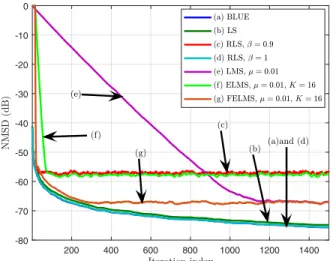
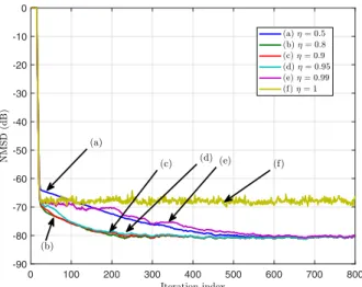
In cases when numerical instability is encountered using the approach in this paper, due to either the use ρ being close to 1 or the drift matrix E being very close to singularity,

İç Mekân Tasarımında Görselleştirme Yöntemleri “Lupa CR29 Projesi Üzerinden Örneklenmesi” 22 tasarım aşamaları bu makale kapsamında örnek olarak

In snowball sampling, an initial group of respondents is selected, usually at random. – After being interviewed, these respondents are asked to identify others who belong to

Also, the results obtained from the random sampling comparison showed that when we compared systematic sampling with random sampling, under the equal conditions (e.g., same number