. Γ·
rf^: Г-
i> s fi,
·*^.’··Γΐ
-i¿
4
W
1
*Ы
'·*
m-
it^ *
Ûtii■ Ш
Й.
î
:,
'
m
'.-* — *» •--¡' ·«»*'«( .^‘
H
Щ ул,
■,
f
■
Τ'
r"·«” -r.f^’Ti. ^ гî"^¡г ı ^ ^
•
‘'· '^'‘*· 1
*“· ’i’*'· ^
'.г
Г7 ’^;
^ .м
^^;·-Г Т
/ 9 3 J f.
A THESIS
S U B M IT T E D T O T H E D E P A R T M E N T O F E L E C T R IC A L A N D
E L E C T R O N IC S E N G IN E E R IN G
A N D T H E IN S T IT U T E O F E N G IN E E R IN G A N D SC IE N C E S
OF B IL K E N T U N IV E R S IT Y
IN P A R T IA L F U L F IL L M E N T O F T H E R E Q U IR E M E N T S
F O R T H E D E G R E E O F
M A S T E R O F SC IE N C E
By
Murat Zeren
September 1994
hiiTiPiA...
taraf
i ' n .y i a / i j : ; j //r .- ¿4 ·^
^ 3 9 4
i
I certify that I have read this thesis and that in my opinion it is fully adequate,
in scope and in quality, as a thesis for the degree of Master of Science.
Prof. Dr. Erol Sezer(Principal Advisor)
I certify that I have read this thesis and that in my opinion it is fully adequate,
in scope and in quality, as a thesis for the degree of Master of Science.
I certify that I have read this thesis and that in my opinion it is fully adequate,
in scope and in quality, as a thesis for the degree of Master of Science.
Assist. Prof. Dr. Billur Barshan
Approved for the Institute of Engineering and Sciences:
Prof. Dr. Mehmet Bar^
ABSTRACT
ADAPTIVE TWO-TIME-SCALE POSITION CONTROL OF
MULTIPLE FLEXIBLE MANIPULATORS
Murat Zeren
M.S. in Electrical and Electronics Engineering
Supervisor: Prof. Dr, Erol Sezer
September 1994
An adaptive self-tuning control scheme is developed in the independent
generalized coordinates for position control of multiple flexible manipulators.
First, a suitable model is derived for multiple cooperating manipulators holding
a common workpiece. Then flexibility is included in the model where each
flexible link is modelled by two rigid sublinks connected by a fictitious joint.
The relatively high stiffness of the flexible links is used to decompose the model
into two subsystems operating at different rates, and a two-time-scale control
is applied to achieve the desired position tracking. Finally adaptive estimation
of the manipulator parameters is proposed to achieve a control scheme which
is suitable for on-line applications.
Keywords :
multiple flexible manipulators, two-time-scale control, adaptive
estimation.
ZAMANLI BİR KONUM DENETİMİ
Murat Zeren
Elektrik ve Elektronik Mühendisliği Bölümü Yüksek Lisans
Tez Yöneticisi: Prof. Dr. Erol Sezer
Eylül 1994
Çok sayıda esnek kolun bağımsız genel koordinatlarda modeli elde edilerek,
konum denetimi için uyarlamalı bir denetim yöntemi geliştirilmiştir. Önce,
ortak bir cismi tutan çok sayıda robot kolu için uygun bir dinamik model
çıkarılmış; ardından, her esnek kol yapay bir eklemle birleştirilmiş iki yarı
koldan oluşmuş varsayılarak, esneklik oluşturulmuş olan bu modele dahil edilmiştir.
Esnek kolların esneme katsayılarının nispeten yüksek oluşundan yararlanılarak,
model farklı hızlarda çalışan iki yarı sisteme ayrıştırılmış ve istenen konum
denetimini sağlamak için iki zamanlı bir denetim uygulanmıştır. Son olarak,
oluşturulan metodun gerçek zamanda uygulanabilirliğini sağlamak için robot
kol parametrelerinin bir kestirim algoritması ile hesaplanması önerilmiştir.
Anahtar kelimeler
hesaplama.
çok sayıda esnek kol, iki zamanli denetim, uyumlu
ACKNOWLEDGMENT
I would like to thank Prof. Dr. M. Erol Sezer for his supervision, guidance,
suggestions and encouragement throughout the development of this thesis.
1 Introduction
1
2 Modelling and Dynamics
8
2.1
Dynamic Model of a Multiple-Joint M anipulator...
8
2.2
Modelling of Multiple Cooperating Manipulators...
11
2.3
Multiple Cooperating Manipulators Having Flexible Links . . .
17
3 A Two-Time-Scale Control Method
20
3.1
Model Decom position... 20
3.2 Control S ch e m e ... 23
3.3
An Adaptive Self-Tuning C o n t r o l ... 25
4 Simulations
28
4.1
Simulation S e t t i n g ... 28
4.2
Simulation R e s u l t s ... 31
5 Conclusion
34
A Simulation Programs
39
B Program Codes
43
VI
List of Figures
2.1
Second-order bulk model of a flexible l i n k
...
17
4.1
Simulation set-up to test the proposed m e t h o d
... 29
4.2
Desired center of mass tr a je c to r y
... 30
4.3
Desired orientation of workpiece in degrees
... 30
4.4
Tracking error in position using true parameters
... 31
4.5
Tracking error in orientation using true param eters
... 32
4.6
Fictitious joint displacements using true parameters
... 32
4.7
Tracking error in position with identification
... 33
4.8
Tracking error on orientation with identification
...
33
4.9
Fictitious joint displacements with identification
...
33
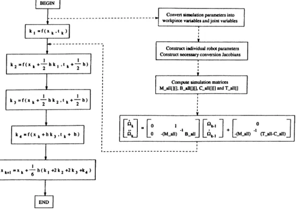
A .l
Flowchart fo r simulation program “rbsp.c”
... 41
A .2
Flowchart for Simulation proced ure
... 42
Introduction
The present age, with the fast and steady progress in science and technology,
has witnessed a large number of new tools developed to make life easy for
mankind. In the field of manufacturing, due in large part to recent advances in
computer technology, a revolution in automation is evolving. Human workers
are being replaced by machines, increasing the productivity and decreasing the
production cost.
Increasingly, production has come to mean the introduction of robots into
the manufacturing environment. Relative to its role in manufacturing, a robot
is defined to be a “reprogrammable multifunctional manipulator designed to
move material, parts, tools or specialized devices through variable programmed
motions for the performance of a variety of tasks” *.
After being introduced as a manufacturing tool, robots started to be em
ployed in various other places like handling of hazardous materials in some
plants, or as remotely controlled manipulators in deep sea or space explo
rations. Though we are still quite far from Isaac Asimov’s human-like robots,
the fact is that robots are gaining more and more importance everyday with
the advances in computer technology and the increase in computing power.
Robotics has appeared as a new field of modern technology. Moreover, this
field crosses the boundaries of traditional engineering, requiring the knowledge
of electrical engineering, mechanical engineering, industrial engineering, com
puter science and mathematics to fully understand the complexity of robots
and their applications.
The expectations from robots and the current trend of technology carried
the research on robotics to many different dimensions. This is where the notion
of multiple cooperating robot arms originated. In fact it is an everyday scenario
which prepares the setting for multiple arms. We, as humans, have two arms
and everyday manual work is normally performed by two-handed humans. In
fact, manual activities and tasks are normally perceived and designed such
that they assume two-handed humans; and if robots are to replace humans in
normal manual activities, it seems natural to visualize and design robots with
two arms and hands. When two or more arms are used to perform a single
task together, as is the case in humans,
increased load carrying, handling
and manipulation capacity can be achieved.
The problem of multiple cooperating robot arms have been studied by many
investigators. To name a few of the recent work in this area; Tarn, Bejczy
and Yun [1] developed a nonlinear control algorithm for multiple robot arms.
They have first derived the Lagrange’s equation of motion for the closed chain
mechanical system by using the Lagrangian of the whole mechanical system.
Obtaining a nonlinear, coupled and complicated model, their proposal was to
linearize and output decouple the system using a nonlinear feedback and a
nonlinear coordinate transformation. Next, cissuming that each robot has a
force/torque sensor installed at its end-effector, they extended this scheme to
force control. Hayati [2] has also developed a position and force control for
coordinated multiple robot arms which eire holding a single object. In this
study, starting with the equation of motion for a single multi-link arm, and
using the fact that the sum of forces at the origin of a compliant frame chosen
by the working environment, and finally he proposed a hybrid control law on
generalized forces to yield position tracking and desired interaction forces. In
a more recent study, Hsu[3] proposed a coordinated control scheme for multi
ple manipulator systems. The objective was to perform a parts-matching tcisk.
Deriving first the dynamic equation of parts matching system and of manipula
tors, he combined all into a complete system equation. Then, a control law on
generalized coordinates was proposed, which could achieve trajectory tracking
as well as achieving the desired internal forces and also the load distribution
to each manipulator according to a weighting factor. The implemented system
and the experimental results were also reported. Another study by Jean and
Fu [5] describes an adaptive control scheme for coordinated multi-manipulator
systems. In this study, they have first derived the so called augmented object
model for cooperating robots, and then using the fact that this dynamic equa
tion formulation is linear in the dynamic parameters of individual robots and
the commonly held object, they converted the dynamic model into a linear re
gression form. Next, modifying the control scheme previously reported by Hsu
[3, 4] to fit their new model, they proposed an adaptive coordinated control.
The method is concluded with a discussion of the convergence properties of the
method. This control, as well eis the one proposed by Hsu, is interesting in the
sense that they facilitated the asymptotic tracking of both the object position
and internal forces without the need for the measurement of contact forces.
Apart from the many studies investigating the coordinated control of mul
tiple manipulator systems, there also exists some other studies investigating
other issues related to multiple manipulator systems. In a study by Li, Tarn
and Bejczy [6], they concentrated on the dynamic workspace analysis of mul
tiple cooperating robot arms. In order to fully utilize the benefits obtained
by the use of multiple manipulators, it is necessary to know the maximum
force/torque that the robots can jointly apply to the environment within their
coupled workspace. This problem was introduced as a maximization problem
and a solution was proposed. As multiple manipulator systems are redundant
in nature, i.e. they have more actuators then degrees of freedom, there exists
some other studies related to optimality on the basis of different cost criteria.
A study by Bobrow, McCarthy and Chu [7] presents an algorithm which min
imizes the time for two robots holding the same workpiece to move along a
given path. Simulation, being an important tool in design and testing of new
control algorithms, hcis also been investigated related to cooperating multiple
manipulators. An example is a study carried out by Murphy, Wen and Saridis
[8], in which the simulation aspects of cooperating robot manipulators on a
mobile platform were investigated.
Putting aside coordinated control of multiple manipulators, another re
search direction appearing with the current trends in robotics is the modelling
and control of lightweight, flexible structures. Lightweight arms are needed to
meet the demands of industry for robots that move faster without requiring
high-powered bulky actuators. As manipulator arms are made lighter their
deformation under stress increases. Thus design of both the mechanical and
control systems require accurate models for simulation and manipulation of
flexible manipulators under a variety of different operating conditions, without
requiring expensive computing machinery.
Based on well-known approaches to analyze the elastic and dynamic be
haviour of flexible structures, a variety of different methods are applied in the
field of flexible robots. A survey on this topic exists in [9]. Generally these
methods can be classified into the following categories:
- kinetostatic methods
- dynamic methods:
The considerations leading to kinetostatic methods start with modelling
the robot as a system of rigid bodies, and due to inertial forces and loads small
elastic deformations are superimposed to the basic rigid body motion. The
elastic deformations of a link in this model correspond to those deformations
induced by external loads applied at proper positions.
In finite element methods, the flexible parts of the robot are modelled by a
finite number of elements, their number depending upon the shape of the part
and the properties attached to an element. In order to describe the vibrations
of the link structure, a mass or better a mass matrix has to be attached to
each finite element. Here this mass matrix can possibly be found by using the
kinetic energy of the element described by a homogeneous mass distribution
and local displacements computed by the nodal displacements and static shape
functions.
As to the vibration mode approach, an analytical description of possible
vibration modes o f a flexible part can be derived directly from the partial dif
ferential equations and the boundary conditions used for the description of
time-spatial bending o f a flexible beam. The main difficulty with this method
lies in choosing the mode shapes and the number of modes that would accu
rately describe link deflections under time-dependent boundary conditions. In
practice, the infinite series that results from solving the Bernoulli-Euler par
tial differential equations is truncated to an arbitrary number of terms. An
experimental study made by Hastings and Book [11] (in which they also used
the separability o f the modes) showed that the frequencies of vibratory modes
in the experiment closely matched the ones in simulation. Here, separability
refers to expanding modes as products of two functions, one being a function
of the spatial variable only and the other being a function of time only.
To handle flexibility, Nemir, Koivo and Kashyap [12] developed the con
cept of a pseudolink. A
pseudolink
is an imaginary line connecting the hub
of a flexible link to its tip. Assuming that the normalized deflection at the
tip is small and that the length of the pseudolink is the same as the length
of undeformed link, they wrote the deflection of the pseudolink as a summa
tion of two terms, one being the true joint displacement and the other being
the angle of pseudolink relative to rigid link position. This second term was
expressed as the weighted sum o f some basis functions which were used to de
scribe the link deflection. It was observed that best results were obtained by
using the Cantilever eigenfunctions as the basis functions. Another study by
King, Gourishankar and Rink [13] made use of this pseudolink concept, and
by decomposing deformations into fast and slow components, they developed a
two-time-scale decoupled control for the end-point position tracking. In a more
recent study by Bodur and Sezer [14], a second order bulk model, consisting
of two rigid sublinks joined by a fictitious joint, is used to approximate the
dynamics of a flexible link. Elastic potential energy stored in the links as they
bend is modeled by the modal stiffness coefficients at the fictitious joints and
a small damping coefficient is also included to account for the damping of the
vibrations. Using the relatively high stiffness of the fictitious joints, the model
is decomposed into two subsystems operating at different rates and a two-time-
scale control is proposed. The proposed scheme is in end-point coordinates and
has the advantage of being adaptive. An experimental study by Yang, Yang
and Kudva [15] considered the load-adaptive control of a single-link flexible
manipulator. In this study, by using a discrete-time ARM A model to describe
the linearized input/output description of the link, they experimented a least
squares identification algorithm and a self-tuning pole placement controller.
proach, the system is decomposed into slow and fast subsystems, and finally, a
two-time-scale adaptive control is proposed. Chapter two explains the deriva
tion of the multiple manipulator dynamics and combines it with flexibility to
derive a general model. Chapter three introduces the model decomposition
and the proposed control, along with the identification technique. Chapter
four is devoted to the simulation results of the proposed control, using two
dual planar manipulators each having one flexible link and holding a common
load. Chapter five gives the conclusions and proposes directions for further
research.
Chapter 2
Modelling and Dynamics
A robot manipulator is in fact a multi-body system. It consists of links which
are connected at the joints with the first link being connected to the base and
the end-point being in touch with the environment to perform a desired task.
Depending on the task to be carried out by the manipulator and the envi
ronment in which it functions, the joints of the manipulator can be prismatic,
allowing linear displacements, or revolute, allowing angular displacements. The
motion is provided by actuators which change the joint displacements so as to
change the position of the end-effector. In order to control this system to
carry out a specific task, we need to have a dynamic model which relates the
torque/force inputs applied at the joints to the resulting displacements at the
joints or the position and the orientation of the end-effector.
2.1
Dynamic Model of a Multiple-Joint Manipulator
Since a manipulator is a mechanical device, the laws governing the motion
of any mechanism is directly applicable to the manipulators.
Principle of
d ’Alembert
states that the sum of all (generalized) torques applied at a joint
should be zero.
Newton’s law
relates net forces to linear acceleration of masses,
whereas
Euler’s law
relates torques to angular velocity and acceleration of a
time, of the
Lagrangian,
which is the difference of kinetic and potential energies.
The equation of motion of a manipulator is obtained using these laws and
the constraints of kinematics. Depending on the evaluation of the equations,
they are called
Euler-Lagrange
(or Lagrangian),
Newton-Euler
or
Generalized
d'Alembert
formulations.
For many applications, the dynamic model can conveniently be obtained
from the Lagrangian function using the Euler-Lagrange equations. Below we
present a brief summary of the derivations of the Euler-Lagrange equations.
Details can be found in [17],[18].
The kinetic energy of the i-th link of an n-link manipulator is given as
1
= jPofliPo.
(
2
.
1
)
where poi is the position vector of the origin of the f-th coordinate frame
attached to the i-th link with respect to the base coordinates and I, is the
pseudo-inertia matrix of the link given as
l i - h i +
7
y , + E i ) ^XiVi IxiZ i P x - r r i i ^XiVi \ { I x i - l y i + h i ) h i Z i p y ^ r u i IxiZ i 2 ( ^ 2 :, + l y i ~~ J z i ) P z i m P x i f r i i p y , m i PziTTli m iI . =
(
2
.
2
)
In equation (2.2), m, is the total mass of the link, p^. =
{PuiPyi^Pzii^Y
is the
center of gravity of the link expressed in its own coordinate frame, and
Ixi = f ( p l
+
p
I )dmi
ly, = U
p
I
-f-
p
I )dmi
h,
= /(p^, +
p], )dmi
Iwv - f PwPvdmi
w
w,v = Xi, Pi,
z,·
(2.3)
10
quantities in equation (2.2) are independent of the positions and velocities of
the joint variables.
The link position vectors in equation (2.1) are related to the joint variables
as
Po,· = A;,e
(2.4)
where A
q
is the homogenous transformation matrix that relates the ¿-th co
ordinate frame to the base coordinate system, and is a function of the joint
variables
0
i ,
62
, · ■ ■ ,
0
i]
and e is a constant vector that picks the last column
of A
q
. Taking the time derivative of both sides of equation (2.4), substituting
in equation (2.1), and summing over all links, the total kinetic energy of the
manipulator is obtained as
T
9
1
, .
i t i \
where tr(·) denotes the trace of the indicated matrix.
* ■ i s f e - ’ i S f ) ’ *'
1 ”
= j E t r
^
1=1
( 2.6)
The total potential energy of the manipulator is simply
n
= - E
(
2
.
6
)
1=1
where the vector g =
[goiigQy,
9
ozi^Y
describes the gravitational acceleration
with components in the directions of the coordinates
{xo,yoiZo)
of the base
coordinate system.
With
C — K —P
denoting the Lagrange energy function of the manipulator,
the equations of motion are obtained by means of Euler-Lagrange’s equations:
dt
d jc { e ,e a )
dOi
dC {d ,9,t)
dOi
= Ti,
i = l , . . . , n .
(2.7)
where
$
=
[
6
i , . .. ,
6
nY
is the vector of joint coordinates and r, is the joint
Now, substituting equations (2.5) and (2.6) in (2.7) we obtain the equation of
motion of the ¿-th link cis
X )
mikqk
+ X X
Cikjjkqj
+
9i
= r,
Jt=l
fc=l j = l
(
2
.
8
)
where
rtiik
=
X
tr
l=max(i,k)
S A L f d A ‘„ '
S
0
i ' { s e t ,
^kj
l=m ax{i,kj)
( d^Al
dOi ‘ ydOkdej^
9i
=
~ X " » i g ^
>5Ai,
■Pi
(2.9)
/=1
In this equation, the first term describes the forces due to the acceleration of
the inertial masses in the system. The second term represents the Coriolis
7^
J)
centripetal
(k = j )
forces. The last term is to account for the
gravitational effect on the motion of joint
i.
As the last step, these equations can be combined into a matrix form and
can be rewritten <is a set of second-order vector differential equation
M (d )^ -fc(tf,6 > )-h g (0 ) =
(2
.10
)where the matrix M is defined to be the mass matrix of robot, c being the
vector o f Coriolis and centrifugal terms, g signifying the effect of gravity and
r being the vector of joint forces/torques.
2.2
Modelling of Multiple Cooperating Manipulators
There exists many settings in which multiple manipulators work and must work
together in a coordinated fashion to accomplish some given task. Often, these
manipulators grasp a single object for the purpose of lifting it, turning it or
carrying it to some other place; forming a closed chain.
12
The first concept that has to be introduced in the formulation of a closed
chain is the number of degrees of freedom.
Degree of freedom
(D.O.F.) of a
system is defined to be the number of independent variables one can pick to de
scribe the entire configuration of the system at hand. In an open chain, D.O.F.
is the same as the number of joints, since each joint can move freely without
any constraint. However, in a closed-chain structure there exists constraints
imposed by the closedness of the system. Thus, D.O.F. is reduced compared
to the sum of D .O .F .’s of individual structures forming the closed chain. A c
cording to the Kutzbach-Grubler criterion [1], the D.O.F. of a spatial linkage
structure with n links each having d/ degrees of freedom, and m joints each
having one degree o f freedom is given as
d
=
ndi — m{di —
1)
(
2
.
11
)
This formulation reflects the fact that each joint of one D.O.F. causes a loss of
{di —
1) D.O.F. for a link.
Let us consider a closed chain formed by
N
manipulators holding a single
object. Assume that
k-th
manipulator has
mk
joints and links. Then the
D.O.F. of the entire system is obtained as
di\Y\mk
+ 1
N
- (di - l ) Y ^ r n k - riN
k=l
N
= Y^TUk + d i - riN
(
2
.
12
)
k=l
where
di
is the D.O.F. of each link and r/, depending on the type of contact,
is the D.O.F. lost at each joint connecting a manipulator to the workpiece.
For a planar configuration
di
= 3, and for a spatial configuration
di =
6.
This means that, we can find a set of
d
independent variables, called the
independent generalized coordinates
to describe the configuration of the entire
system. In [1], the dynamics of the closed-chain mechanical system was derived
by obtaining the Lagrangian of the whole system and applying the Euler-
Lagrange equations to get the system equation in generalized coordinates and
generalized forces. Though being quite automatic, the interaction forces never
appear in this formulation. Here, a different approeich is taken to derive the
dynamics of the individual parts in the system, viewing the interaction forces
as well.
Let
dkik
= 1 ,...,A ^ , be the joint variables defining the position of fbth
manipulator and similarly
B
q
be an equivalent set defining the position of the
commonly held object. The Cartesian position o f some point p in the object
can be written as a function of the object coordinates
B
q
alone, p = p(0o)> or
as a function of the end-effector position of any arm and the orientation of the
work-piece, i.e..
p W = PJt(^fc,^o),
A: = 1 , 2 , . . . , TV
(2.13)
These closure equations represent the geometric constraints on the system.
Differentiating the above closure equations with respect to time gives
Jo^o —
k —
1 , 2 , . . . , TV
(2.14)
where Jo is the Jacobian of p(^o) with respect to
B
q
\
Jjt, the Jacobian of pjt
with respect to
Bk'·,
and Jojt, the Jacobian of p* with respect to ^o·
With these in mind, view the robot arms and the object
as
separate me
chanical systems. The equations of motion for these mechanical systems have
the form
= 'Tfc-1-V)t,
A: = 1,...,TV
(2.15)
for the robots, where Mjt’s eire the mass matrices and hjt’s collect the Coriolis,
centrifugal and gravity terms. Here rjt denotes the joint forces/torques in the
A:th system and v* represent the generalized interaction forces acting on the
Arth system. The equations o f motion for the object is given by.
Mo(^o)^o + ho(^O)^o) — Vo
(2.16)
14
is moved only by interaction forces rather than the independent force/torque
drives. The coupling among the above equations is obtained through vjt’s.
In order to relate the constraint forces to the dynamics o f the system, we
use the fact that constraint forces do no work. Defining, v = [
vq
,
v j ,
· · ·,
and
6
= [
0
Q, d j,
· · ·,
we have,
= 0
(2.17)
for all admissible velocities
9.
If there were no constraints on the individual
systems, as is in the open-chain case, the velocities
9k
of each system could
vary arbitrarily and the above equation shows that the forces of interaction,
Vjt, would be zero.
The joint velocities
9
must also satisfy the constraints in equation (2.14),
or putting them into matrix form
where.
j ( « ) =
3 (в )в
= 0
Jo ~ Joi
—J l
Jo ~ JoAT
(2.18)
- J
N
Now, equation (2.18) shows that
9
is in the null space of J(^ ), and equation
(2.17) shows that v is orthogonal to
9.
Thus, we conclude that v is in the range
space of J^(^) or that, there exists a vector f / 0 such that.
V = J ^ (^ )f .
(2.19)
Here f represents the internal forces built in the closed chain mechanical
system. If we partition f as f = [fT", · · ·, f^]^, with
fk,k =
1
, . . . ,N
representing
the internal forces acting on the tip of each robot, individual system equations
for each robot can be written as
and for the object eis
M
q
^
o
+ ho(^O) ^o) — Jw)f
where
J
qo
—
[(Jo ~ Joi) г ■ ■ 5 (Jo ~ Joлг) ]
ТлТ
(
2
.
21
)
Now, let’s pick a set q of d independent generalized coordinates describ
ing the configuration of the whole system, where
d
is the D.O.F. of the sys
tem. Then, we know that, since the knowledge of q determines the configu
ration of the whole system, they also uniquely determine the joint variables
it = 0 , 1 , . . . ,
So, we have a relation of the form
В к =
6>fc(q)
(
2
.
22
)
for each subsystem. Here, it is worth mentioning that while choosing the set
q, our main concern is the type of control problem we have at hand. For a
position tracking problem, it is desirable to put the variables to be controlled
into set q.
Next, we convert the dynamic equations of individual subsystems given in
their own joint coordinates into generalized coordinates using the derivatives
of equation (2.22) as
= J^ *(q)q
Ok =
J ^ jt(q )q -f j^ jt(q ,q )q ,
k = l , . . . , N
(2.23)
where
is the Jacobian of
$k
with respect to
q,
and
J^^
is an njt x d matrix
with the
{i,j)-th
element given as
J2i=i
Inserting these into equations
(2.20) and (2.21) above, we have
Mit(q)q + hi(q,q) = T)t-Jfcf)t,
k = l , . . . , N
(2.24)
Mo(q)q + ho(q, q) = Joof
(2-25)
16
M ,(q ) = M , ( 0 , ( q ) ) J ^ , ( q )
hfc(q,q) = hjfe (©jt(q),J^j^(q)q)+Mfc(©it(q)) j^j^(q,q)q,
A; = 0,1,..., A^.
Now, we have all the dynamics formulated in the generalized coordinates. To
proceed, note that the matrix J
qo
is nonsquare and is in fact of full column
rank. So, using the pseudo-inverse of J
qo
, we solve for the minimum norm f
from equation (2.25) as
f = (Joo)^[Mo(q)q + ho(q, q)]
(2.26)
where
(j^o)^ = J
oo
(J2
o
J
oo
) - '
This f vector is that particular f vector which achieves the positioning of the
workpiece without building extra internal forces on it, and thus the f vector
which we will use in constructing the computed torque input. With (Jo^)]t
denoting the
k-th
block row of (J2o)^ we have
fit = ( j M ( M o ( q ) q + ho(q,q)]
Finally, substituting this into equation (2.24),
M jt(q)q + hfc(q,q) = rjt,
k = l , . . . , N
(2.27)
(2.28)
where
M , = M it(q) + Jr(Joo)iM o(q)
hfc(q,q) = hjt(q,q) +Jf(jM M q,q)
Combing these final system equations of individual robots into a larger matrix
formulation, we obtain
(2.29)
■ M ,(q ) ■
h i(q ,q )
Tl
•
q +
•
•
. M ^ (q ) _
. hAi(q,q) _
TN
_
or simply
M(q)q-t-h(q,q) = r
(2.30)
2.3
Multiple Cooperating Manipulators Having Flexi
ble Links
As introduced earlier, the need in the industry for lightweight manipulators
resulted in the production of robots with flexible links. To solve the problem
of dynamic modelling of these links various methods have been proposed. In
this section, a modelling scheme for multiple manipulators having flexible links
is discussed. The dynamics of a flexible link is approximated by a second-order
bulk model, which consists of two rigid sublinks joined by a fictitious joint as
in [14] and [16]. In this model, the angular displacement of the fictitious joint
is a measure of the deflection of the link. Elastic potential energy stored in
the links as they bend is modelled by the modal stiffness coefficients at the
fictitious joints, and a small damping coefficient is also included to account for
the damping of the vibrations.
Let’s consider a single manipulator consisting of
n
links,
r
of which are
flexible. If we model these links by a second-order bulk model as described
above, the dynamical model of such a manipulator can easily be obtained by
18
using the Euler-Lagrange equations as
0
+ c{
0
,
6
,
0
,
6
) + g{
0
,
6
) =
^^0
6
(2.31)
where
0
G R " are the true joint displacements and 6 G R ’’ are the fictitious
joint displacements. The actuator forces/torques are external inputs to the
system and are collected in
t q
.
The torques of fictitious joints, however, are
determined by the internal dynamics of the flexible link as
(2.32)
where K , =
diag{Kai,· · · iKar]
and K j =
diag{Kd\■,■··■,Kdr)
contain the
spring constants and the viscous dampings of the fictitious joints, respectively.
This model is quite simple and can easily be combined with the model
obtained in equation (2.30). One point that needs to be clarified is, perhaps,
the modification in q, the independent generalized coordinates. Set q can still
assume the form it had before the introduction of flexibility, but this time the
fictitious joint variables coming from all the flexible links should be appended
to the end of this vector. This, in fact, is the same thing that we would
have expected if we had added extra true joints with independent actuators.
Since an extra joint increases the D.O.F. of the system by one, the number of
independent generalized coordinates should also increase by one.
When flexibility is included, equation (2.20) is modified into
Mfc
Ok
Ok
+
^k{Ok,Ok,
0
k,Ok)
=
I'^Sk 1
Jjfk,
k = l , . . . , N
(2.33)
and the equation (2.23) is modified into
Ok
^
0
k h k
q
Ok
_
0
I* .
6
(2.34)
' вк
_
^ вк ^ 6k
q
+
^¿ijt
q
. 0
I* .
6
0
0
6
,Ar = l,...,7V (2.35)
where
and the matrix Ijt being a matrix which is of the form
Ifc = [0 I 0] where the identity matrix I picks the entries from
6
corresponding
to
6
k-With these modifications, going through the similar steps in construction
o f the combined system equation and after a suitable reordering, we have
(2.36)
M { q ,
6
)
q
+ h(q,^,q,^) =
6
Chapter 3
A Two-Time-Scale Control Method
Accurate positioning of the end-effector is an important issue in robot con
trol systems. Especially, in manipulators having flexible links, this problem
becomes more challenging since flexibility induces high frequency vibrations
which are difBcult to control and should be damped at the end of the trajec
tory as soon as possible. While deriving the control law, it is assumed that
the pseudo-joint angles can be constructed from the strain gage measurements
positioned along the link as in [12].
3.1
Model Decomposition
In the position control of multiple coordinated manipulators, if flexibility is
included, the desired motion to be performed by the manipulator system is
much slower in nature when compared to the oscillations due to flexibility.
Though many schemes have been proposed to control the relatively slow de
sired motion, still special care should be given to prevent these high frequency
oscillations. Facilitated by the relatively high stiffness of the flexible links, the
method proposed here makes use of the decomposition of the system model
into two reduced order models operating at different rates. Once we have this
multi-time-scale model, we can implement a suitable control at each time scale.
Let’s cissume a model in which we have n joint actuators(external inputs),
d
independent generalized coordinates(D.O.F.) and
r
flexible links-thus r extra
generalized coordinates. The two-time-scale scheme described below applies
to the case where
r < d.
Otherwise, a multi-time-scale decomposition and a
suitable control should be applied by a proper ordering of the diagonal elements
of stiffness coefficients matrix, K ,.
Let’s start by partitioning the matrices in equation (2.36) resulting in,
M„a
iqq
q
+
h q ·
_
é
> 5 .
. ^6 .
(3.1)
where M „ € R ” '"',
€ R ’·'“", M j , € R "'·',
Mgg
€ R " " , h , € R ” and
€ R ’’. While deriving the two-time-scale decomposition, we assume that
q is a slow(quasi constant) variable but that
6
consists of both slow and fast
parts. Here, we make use of the fact that K , is a relatively large quantity and
write it as
with
/i
small and K ' approximately at the same order
as the other parameters in the model.Next, we apply singular perturbations
technique to derive the decomposition. However, as M is non-square it is not
invertible and we cannot bring the equations into the standard state space form
X = f ( x ,z , u ,/i,i)
fii
= g ( x ,z ,u ,/i ,i )
(3.2)
of a singularly perturbed system([22]). Instead, we first write equation (3.1) as
M qqq -I-
+ hq = Tq
+
^ 6 6 ^
+
= 0
and introduce the state variables
Xi = q,
X
2
= 4
=
^r‘^
6
,
Z
2
=
which are decomposed into fast and slow components as
X j ~ x , ,
Z, ~ Z , + Zj,
> = 1,2 ,
T , ~ r q + f q
(3.5)
(3.3)
22
with bar denoting slow components and hat denoting fast components.
With the above state variable assignment, equation (3.3) is changed to
Xl = X2,
MqqX2 + ^Mq^Z2 + hq
= Tq,
f l i l =
Z
2
,
+ K 'Z i + /iKrfZ2 = 0
(3.6)
(3.7)
(3.8)
(3.9)
Now, the slow components of z ,,i = 1,2 can be solved from the equations
(3.8) and (3.9) with ^ = 0 as.
Zl = - ( K ; ) * (M^qX2 + h^)
¿2 = 0
(3.10)
By using equations (3.6) and (3.7) with /i = 0, the slow components of x, are
shown to satisfy
Xl = X2
NiqqX2 "f· hq
— Tq
(3.11)
To obtain the fast dynamics(boundary layer system), we first solve for X
2
from
equation (3.9) and substitute it into (3.7). Next, we apply the last phase of
the singular perturbations method to get the fast dynamics. While solving for
X
2
from equation (3.9), since we assumed
r < d at
the beginning,
is of
full row rank. So, let’s use the pseudo-inverse of
to get
¿ 2
as
X, =
+
k
;
z
, + /iK jz j)
(3.12)
where.
,
- 1
Next, we insert this in equation (3.7), switch to the fast time scale by defining
a fast time variable
(3.13)
and finally substitute // = 0. Eliminating the slow quantities, the dynamics of
the fast subsystem in the original time variable
t
is obtained as
H
¿2
~ MqqM^^K^Zj = fq
(3.14)
Going back to the true variables from state variables, we have
Mqq<4 "k hq —
Tq
(
m
, 5 -
I
-
= f .
(3.15)
(3.16)
(3.17)
describing the slow and fast dynamics of the multiple manipulator system.
3.2
Control Scheme
The above decomposition of dynamics into slow and fast components is valid
only if the fast subsystem in equation (3.16) is asymptotically stable([22]). If
the fast subsystem can be stabilized for any trajectory of interest, the overall
system approaches in the limit to the reduced order decomposition. Thus, we
first stabilize
6
by applying a fast feedback of the form
Tq =
+
Kp6
Kp =
-M qqM
equation (3.19) is reduced to
6
"k Zjtf + Z2^ — 0
(3.18)
which, when combined with the model equation (3.16), results in
( M , i -
I - i c i - (
m
<,,
m
^^
k
, + K , ) « = 0
(3.19)
From equation (3.19) we observe that, if we let
K . = - ( M , i -
z .
' ('^<1« ■■
Z ,
(3.20)
24
Now, Zi and Z
2
can be chosen arbitrarily to stabilize the fast subsystem by
placing its 2r poles at desired locations. Note that this also allows for the
decoupling of fast dynamics, meaning that the vibrational modes associated
with the fictitious joints can be controlled independently.
With the fast subsystem stabilized, it now remains to choose the slow com
ponents of the slow subsystem defined in equation (3.15). This is the standard
tracking problem of rigid manipulators. A computed torque type control can
be chosen, in which we feedforward the slow control to achieve the desired
trajectory along with a feedback control to compensate for the deviations. So,
the slow control takes the form
Tq — IVIqqij -|- hq -f- K „e q T KpOq
(3.22)
where q'^(t) describes the desired trajectory in terms of the independent gen
eralized coordinates and eq = q “* — q is the deviation of the actual trajectory
from the desired one. Application of this control results in the error dynamics
given by,
Mqq6q -f- KvGq -f KpCq = 0
(3.23)
Letting,
K „ = M qqZi
Kp = MqqZ2
(3.24)
equation (3.23) is reduced to
6q -f- Zi6q -f- Z2Cq — 0
(3.25)
Clearly, Zj and Z
2
can be chosen properly to place the
2d
poles of the slow
subsystem as desired. Again, choosing Zj and
¿ 2
in a diagonal form decouples
the error dynamics of generalized coordinates.
The composite control is the sum of fast and slow controls in equations
control. Since
6
is not directly measurable, it somehow has to be computed.
Since
6
is measurable and
6
can be computed from equation (3.17),
6
is com
puted using
6 c:i 6 — 6.
Also using ^ = 0, which comes from equation (3.10),
6
is computed by using
6
6.
So, the fast control finally takes the form.
f , =
K j
+ Kp ( i +
k
; ·
+ h^))
which, like the slow control Tq, involves only available variables.
(3.26)
While implementing the control law in discrete-time, or possibly on a digital
computer, most probably time derivatives of the true-joint and pseudo-joint
variables will not be available to us but rather the values of the variables at
sampling instants. The time derivatives in this case can be computed using
backward differencing like
Xk
=
T~^Axk
and
Xk = T~^A^Xk
where
T
is the
sampling period,
Xk
is the value of the variable
x
at A;th sampling instant and
A is the backward difference operator defined by Axjt
= Xk —
X k - \ ·3.3
A n Adaptive Self-Tuning Control
Implementation of the control law derived in the previous section requires that
the system parameters Mqq,
hq and
be known. Though
they can be computed analytically, these parameters are highly nonlinear, in
volving lots of sines and cosines, and these extensive computations are not
suitable for on-line applications.
An alternative to computing the manipulator parameters is to estimate
them from input/output data using an adaptive estimation algorithm and then
base the control law on the estimated parameters. The Recursive Least Squares
Estimation (RLSE) algorithm ([21]) is a suitable method to use in identification
since it has a low computational complexity due to being recursive, and also a
fast convergence.
26
For the development of the identification algorithm, we use the model de
rived in equation (2.36). Define j? = [q^
6^Y
and r =
[
t
^
t
^]^· Scaling the
equation with
a,
equation (2.36) can be rewritten as,
a r = [M ah]
a f i
1
(3.27)
Here,
a
is incorporated as a scaling factor to increase the numeric precision of
the algorithm. Also, as
Q
will not be available to us but rather the sampled
values of i? only, i? can be approximated by backward differencing as i? =
T~^A^i2k.
Here, again
T
is the sampling period, Д is the backward difference
operator and
denoted the sampled values of i?. At this point we can choose
a — T
which brings the parameters o f above formulation to about same order.
Letting,
У к = Т - T k , Ф к
=
1
л-fc = [Mjk rhfc]
(3.28)
where the subscript
k
is to denote the values at the A:th sampling instant with
<l>k
being the observation vector(regressors) and
tt
* being the parameter matrix,
equation (3.27) can be written in the standard form
y* =
'>^кФк
(3.29)
Assuming slow variations of parameters, a least-squares estimate of TTjt
which minimizes the weighted sum
Л = ¿
7
''
Ч
у
I - ^1Ф1У(У1 - ^¡Фд
1=0
(3.30)
is obtained in [21] as
Ok =
Pk =
(1
+
< - i +a t ( y t - ж
1
_ , ф , , ) ф [ Р
1
, . ,
(3.31)
where superscript e denotes the identified parameter matrix. Once
TTk
is calcu
lated, M t and hfc are determined and then are suitably partitioned to compute
the next control inputs. The system parameters required for the construction
of the fast and slow controls in the
(k
-|- l)st iteration are replaced by their
estimates computed at the ¿th iteration.
In implementation of the RLSE algorithm, the initial value of
can be
given by either calculating it once and for all to initiate the algorithm, or can
be suitably chosen based on the a priori information about the system. In
choosing the initial value of Pjt, the common practice is to choose it as A · I
with A > 0 and I being the identity matrix.
Chapter 4
Simulations
A simulation study has been carried out to test the effectiveness of the pro
posed adaptive two-time-scale control method. A simulation program has been
written in C and run on SUN-Sparc 10 workstations.
4.1
Simulation Setting
The simulation set-up consists of two planar two-link dual manipulators. The
manipulators have one rigid link connected to the base and one flexible link
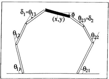
each, and are holding a rigid workpiece at both ends as shown in Fig. 4.1.
In the simulation set-up, the links of the manipulator are all 0.5 m long and
have masses 10
kg
each. The effective inertias and damping coefficients of the
actuators are 6.35
kg.m^
and 2.12
N.m.s.
for the first joint and 1.30
kg.m^
and
0.43
N.m.s.
for the second joint. The two manipulators are spaced by 1.0 m.
The commonly held workpiece is 0.2 m long and is 10
also.
Each flexible link is modelled by a second-order bulk model approximation,
consisting of two sublinks having lengths 0.25 m each. On the assumption
that the flexible link is homogeneous, the mass of the flexible link is equally
distributed between the two links
as 5 kg
each. The spring constants and the
Figure 4.1:
Simulation set-up to test the proposed method
damping coefficients of the fictitious joints are assumed to be
=
400
N.m
and
Kd
= 10
N.m.s,
respectively. Note that the assumed value of
Kg
is large
enough to justify a singularly perturbed model.
The closed chain configuration in Fig. 4.1 has 7 links each having a D.O.F
di =
3, and 8 joints. Thus the D.O.F. of the entire configuration is
d = 3 x 7 - 2 x 8 = 5
We choose as generalized coordinates the Cartesian x and y coordinates of the
center of mass of the workpiece, its orientation angle
<j>,
and the pseudo-joint
angles of the flexible links, totaling 5.
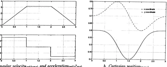
The desired trajectory is given in terms of the three variables associated
with the workpiece. The trajectory to be followed by the center of mass of the
workpiece is a circular path in the plane of the workpiece with radius 0.1 m
and centered at (0.5 m ,0.7 m). It is to be traced in 3 s starting from the
point (0.6 m ,0.7 m ), with an angular velocity and acceleration as specified in
Fig. 4.2.a. Corresponding displacements of the center of mass in Cartesian
coordinates are shown in Fig. 4.2.b. While this trajectory is being traced by
the center of mass of the workpiece, the orientation angle of the workpiece is
desired to trace a sine wave as shown in Fig. 4.3. This trajectory contains large
inertial variations along the path, and is chosen to demonstrate the effectiveness
30
O 0.5 1 1.5 2 2.5 3
a. Angular
üe/ociijtnd/.v..)
and
acce/eraiion(r»d/**v..)
Figure 4.2:
Desired center of mass trajectory
Figure 4.3:
Desired orientation of workpiece in degrees
of the proposed method.
The simulations are performed by modelling all the links as homogeneous
structures with center of masses at their midpoints. A point-mass model is used
for the links and their rotational inertias are computed on the homogeneity as
sumption. In simulations a discrete model of the manipulator corresponding
to a sampling period of T = 0.005
s
is used. That is, the manipulator param
eters are updated(either by calculation or estimation) once every 0.005 s, as
well as the value of the control input. Runge-Kutta method with a step size
oi h =
0.001
s
is used for numerical integration of the manipulator equations
during each sampling period.
b. Along y-axis
Figure 4.4:
Tracking error in the position o f center o f mass using true
parameters (m vss)
4.2
Simulation Results
In the simulation, K „ and Kp are selected to place the poles of the error
equation (3.25) at s i
,2
= —20 for the slow subsystem. By a proper choice of
A A